Article

Effect of Vertical Wind Shear on PM2.5 Changes over a Receptor Region in Central China

1
Collaborative Innovation Center on Forecast and Evaluation of Meteorological Disasters, Key Laboratory for Aerosol-Cloud-Precipitation of China Meteorological Administration, Nanjing University of Information Science and Technology, Nanjing 210044, China
2
Institute of Heavy Rain, China Meteorological Administration, Wuhan 430205, China
3
Changsha Meteorological Bureau, Changsha 410205, China
4
Jingmen Meteorological Bureau, Jingmen 448000, China
*
Author to whom correspondence should be addressed.
Remote Sens. 2022, 14(14), 3333; https://doi.org/10.3390/rs14143333
Submission received: 2 June 2022 / Revised: 29 June 2022 / Accepted: 7 July 2022 / Published: 11 July 2022
(This article belongs to the Section Atmospheric Remote Sensing)

Abstract

:
Vertical wind shear (VWS) significantly impacts the vertical mixing of air pollutants and leads to changes in near-surface air pollutants. We focused on Changsha (CS) and Jingmen (JM), the upstream and downstream urban sites of a receptor region in central China, to explore the impact of VWS on surface PM2.5 changes using 5-year wintertime observations and simulations from 2016–2020. The surface PM2.5 concentration was lower in CS with higher anthropogenic PM2.5 emissions than in JM, and the correlation between wind speed and PM2.5 was negative for clean conditions and positive for polluted conditions in both two sites. The difference in the correlation pattern of surface PM2.5 and VWS between CS and JM might be due to the different influences of regional PM2.5 transport and boundary layer dynamics. In downstream CS, the weak wind and VWS in the height of 1–2 km stabilized the ABL under polluted conditions, and strong northerly wind accompanied by enhanced VWS above 2 km favored the long-range transport of air pollutants. In upstream JM, local circulation and long-range PM2.5 transport co-determined the positive correlation between VWS and PM2.5 concentrations. Prevailed northerly wind disrupted the local circulation and enhanced the surface PM2.5 concentrations under polluted conditions, which tend to be an indicator of regional transport of air pollutants. The potential contribution source maps calculated from WRF-FLEXPART simulations also confirmed the more significant contribution of regional PM2.5 transport to the PM2.5 pollution in upstream region JM. By comparing the vertical profiles of meteorological parameters for typical transport- and local-type pollution days, the northerly wind prevailed throughout the ABL with stronger wind speed and VWS in transport-type pollution days, favoring the vertical mixing of transported air pollutants, in sharp contrast to the weak wind conditions in local-type pollution days. This study provided the evidence that PM2.5 pollution in the Twain-Hu Basin was affected by long-distance transport with different features at upstream and downstream sites, improving the understanding of the air pollutant source–receptor relationship in air quality changes with regional transport of air pollutants.

Graphical Abstract

1. Introduction

Air pollution with high PM2.5 concentrations in the ambient atmosphere has been a crucial problem in environmental science [1,2], with adverse influences on climate change and human health [3,4]. The PM2.5 variations, causes, and impacts have been intensively studied over recent decades [5].
PM2.5 changes are co-determined by anthropogenic emissions and meteorological conditions [6,7]. In response to the severe air pollution, the Chinese government issued the Action Plan on Prevention and Control of Air Pollution in 2013, imposing emission control on industry production, vehicles, and energy consumption [5,8,9]. The meteorological conditions significantly influence the formation and evolution of air pollution and offset the emission reduction efforts in some years [10,11,12]. Local accumulation, chemical transformation, and long-range transport are key factors of air pollution [13,14]. The stagnant meteorological conditions, such as low atmospheric boundary layer (ABL) height, strong temperature inversion, weak near-surface wind, and high relative humidity, are unfavorable for the dispersion of air pollutants [14,15]. The formation of secondary aerosols and aerosol–ABL interactions play vital roles in the explosion of air pollution under stagnant weather conditions and weakening monsoons [16,17,18,19,20]. In addition, the regional transport of air pollutants is a remarkable contributor to regional air pollution events [10,21,22]. However, it is difficult to figure out the associations between vertical wind structures in ABL and PM2.5 concentrations due to the lack of credible observations in local wind profiles.
Radar wind profilers (RWPs), generally Doppler radar, have been widely applied to monitor the vertical structures of meteorology with high temporal–spatial resolutions, especially in ABL [23,24,25]. Ground-based RWP can remotely monitor vertical and horizontal winds as well as mix processes to identify the meteorological conditions in the lower troposphere and explore the dynamic features of ABL [26,27,28]. Furthermore, synchronous observations and model simulations are the most common methods to analyze ABL structures, revealing the vital role of vertical wind changes in modulating air pollution [29,30]. To date, a large number of field campaigns involving the wind profiles observed using RWP have been conducted, especially over megacities, and the archived dataset has received increasing attention [28,31,32,33].
Air pollution in the Twain-Hu Basin (THB), featuring the lower plain in Hubei and Hunan provinces over central China, has become a heavy pollution center in recent years [34,35,36]. THB is located in the downwind areas of heavy air pollution in north and east China, serving as a key receptor region in the regional transport of air pollutants from upstream regions driven by East Asian monsoonal winds [34,37]. Heavy air pollution with a unique “non-stagnation” ABL in THB is aggravated by regional PM2.5 transport [38,39], and the effect of meteorology on PM2.5 pollution can accelerate and offset the effects of emission reductions oppositely in the northern and southern THB, respectively [40]. However, there is few research on the impact of vertical wind shear (VWS) on PM2.5 pollution over the receptor region in central China. Based on high-resolution radar observation, and surface environmental and meteorological observations in winters from 2016–2020, our study aimed to investigate the impacts of VWS on surface PM2.5 concentrations in two representative urban sites, Changsha (CS) and Jingmen (JM), in the southern and northern THB, respectively, and to reveal the implication of regional PM2.5 transport for environmental changes.

2. Data and Methods

2.1. Data

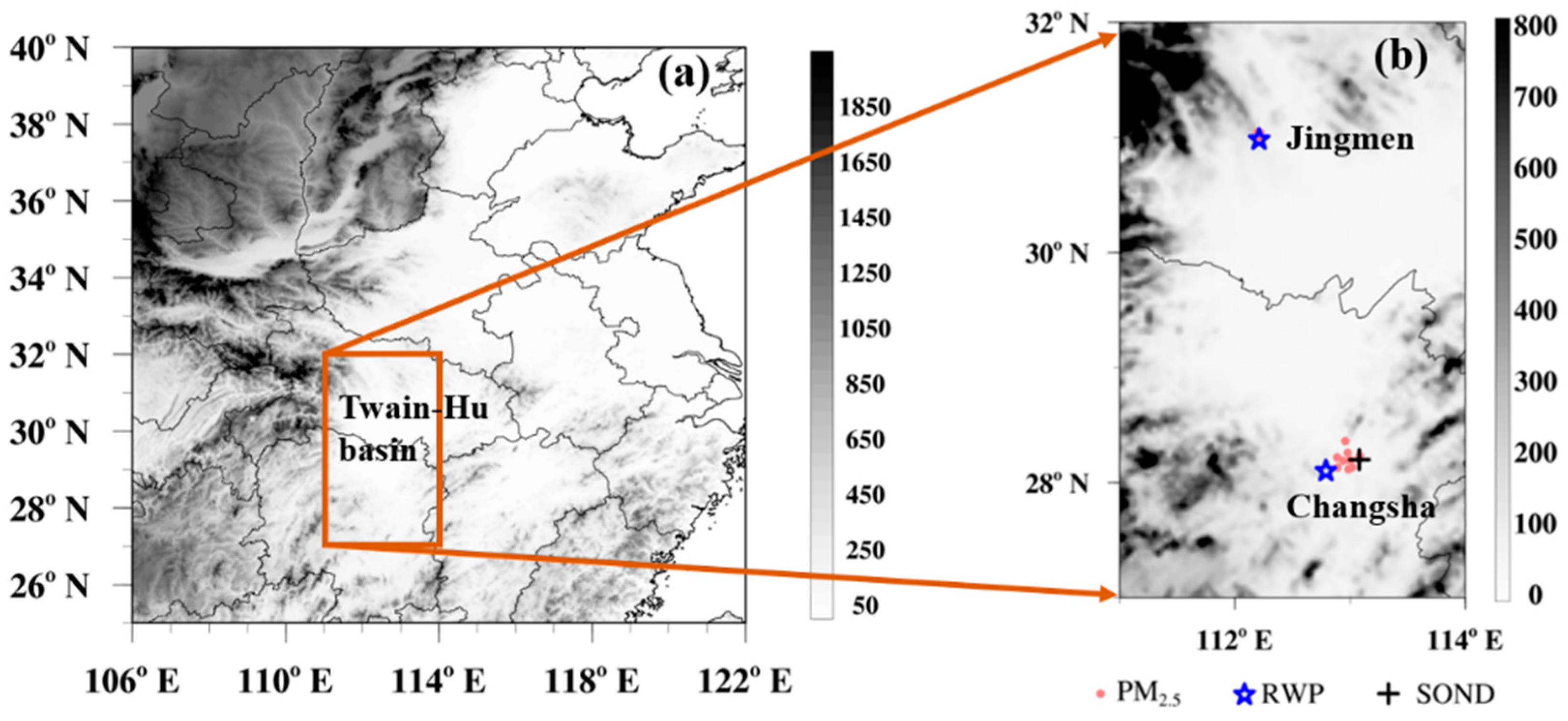
2.1.1. Ground-Based Meteorological and Environmental Data

The observational data of hourly PM2.5 concentrations in CS and JM (marked by pink dots in Figure 1b) for boreal winters (December, January, and February) from 2016–2020 were collected from the national air quality monitoring network [41], which was under strict quality control based on China’s national standard of air quality observation. To avoid the uncertainties induced by heterogeneous aerosol distribution among different sites in the same city, hourly PM2.5 concentrations for CS and JM were averaged with no more than 50% missing data over 10 and 4 environmental observation sites, respectively. The contemporaneous hourly meteorological data were sourced from the weather monitoring network of the China Meteorological Administration [42], including wind speed and wind direction.

2.1.2. RWP and Radiosonde Measurements

The RWP data were collected in CS and JM (marked by blue pentacles in Figure 1b), including the profiles of horizontal wind speed and direction. The raw data have undergone strict quality control before further analysis [31,43]. Hourly averaged wind profiles were computed from the original 6 min RWP data to match hourly PM2.5 concentrations, with no more than 40% missing data. On account of the high missing rate of RWP data above 1000m, the subsequent analysis of vertical wind was only conducted under 1000 m in JM to ensure the continuity and sample capability of vertical wind data (Figure S1).
The radiosonde sounding data measured in CS were used to characterize the thermodynamic structure relevant to air pollution. The sounding balloons are launched twice per day at 08:00 and 20:00 local standard time (LST, UTC+8). The detailed information on RWPs and radiosonde measurements are presented in Table 1.

2.2. Methods

For all measurements mentioned in this study, only the non-precipitation hours were selected to eliminate the effect of wet deposition on air pollutants. The precipitation hours are defined with precipitation amounts >0.1 mm [44]. Hourly PM2.5 concentration was normalized with monthly average [45], and the normalized PM2.5 concentration was grouped into three subsets with the same sample number [32]. The lower (bottom 1/3) and upper (top 1/3) terciles of the normalized hourly PM2.5 refer to clean and polluted conditions, respectively, to ensure that comparison can be performed with the same sample number between clean and polluted conditions [32].
VWS is an important indicator of dynamically vertical mixing [32]. Hourly VWS is calculated with a 120 m vertical resolution. The bulk VWS is used to characterize the intensity of wind shear between two heights, which refers to the magnitude of bulk vector difference (top minus bottom) divided by height [32,46], expressed as follows:
VWS = ( u z 1 u z 2 ) 2 + ( v z 1 v z 2 ) 2 ( z 1 z 2 ) × 1000
where VWS is the vertical wind shear (unit: m s–1 km–1). u z 1 and u z 2 are the zonal wind at the height of z 1 and z 2 , respectively, and v z 1 and v z 2 are the meridional wind at the height of z 1 and z 2 . z 1 is the top height and z 2 is the bottom height.

2.3. WRF-FLEXPART Modeling

2.3.1. Model Description

The Lagrangian Flexible Particle dispersion model (FLEXPART) was initially used for calculating long-range and mesoscale dispersion of air pollutants from point sources. For the fine and further multi-scale modeling, a FLEXPART version worked with Weather Research and Forecasting (WRF) mesoscale meteorological model (WRF-FLEXPART version 3.1) was released [47]. In the WRF-FLEXPART model, the trajectory of abundant particles released from a source is simulated, considering the processes of horizontal transport, turbulent diffusion, and wet and dry depositions in the atmosphere [39,47], which has been widely used to determine the potential sources of air pollutants [39,48].

2.3.2. WRF Modeling Configuration and Meteorological Validation

In this study, WRF version 4.0 was employed using two nesting domains with horizontal resolutions of 30 and 10 km, covering most Asian regions and China (Figure S2). The physical parameterizations included the Noah land surface model, Grell 3D cumulus parameterization [49], the Mesoscale Model (MM5) similarity surface layer, the Yonsei University (YSU) boundary layer scheme [50], the Rapid Radiative Transfer Model (RRTM) longwave scheme [51], the Goddard shortwave scheme [52], and the Lin microphysics scheme [53]. Initial and boundary meteorological conditions were driven by the reanalysis meteorological data in the horizontal resolutions of 1° × 1° obtained from NCEP [54].
The simulated meteorological fields for winters from 2016–2020, including pressure (P), air temperature (T), relative humidity (RH), and wind speed (WS), were compared with observations in CS and JM, and the evaluation results are listed in Table S1. The simulated T, P, and WS were slightly overestimated in CS, and the simulated T, RH, and WS were slightly underestimated in JM with high correlation coefficients (over 0.60). The RMSEs were determined to be low with NMBs and NMEs less than 30% and 50% in two sites, which were comparable to other modeling studies falling within the “good” or “satisfactory” criteria [55,56]. According to the statistical results, the WRF modeling meteorology was reasonably consistent with observations, which could further drive the FLEXPART simulation.

2.3.3. Estimation of the Contribution of Regional PM2.5 Transport

In FLEXPART modeling, a large number of particles are released at a receptor site and transported backward, and then, the residence time of all particles on each grid is normalized by the total number of released particles [39,47]. In this study, the simulation of 48 h backward trajectory was conducted with the release of 50,000 particles from CS and JM for winters from 2016–2020. The residence time of air particles was output with a horizontal resolution of 0.1° × 0.1°. The residence time (units: s) over the backward trajectory pathways was multiplied with primary PM2.5 emission fluxes (units: μg m–2 s–1) to quantify the emission source contribution from the grid cell to the PM2.5 changes in receptor [39,57,58,59]. The primary PM2.5 emission data in this study are obtained from the Multi-resolution Emission Inventory for China (MEIC) in 2016 [60]. The detailed methods are described by Yu et al. [39].

3. Results and Discussion

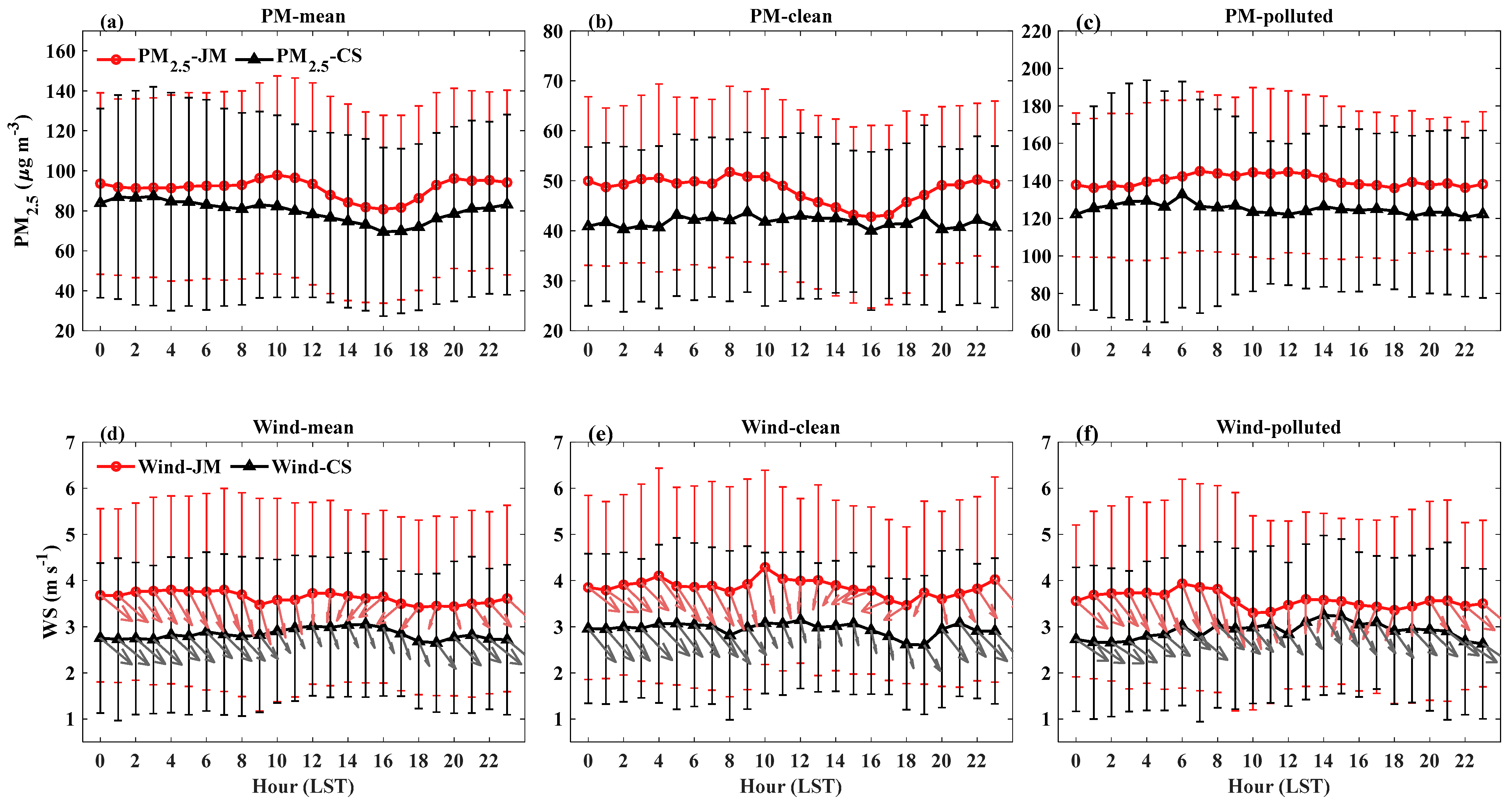
3.1. Wintertime Variations in Surface Conditions

JM and CS are located in the northern and southern THB, upstream and downstream regions of the southward transport pathway driven by East Asian winter monsoon. The diurnal variations in PM2.5 concentration were generally consistent in JM and CS, and exhibited a pattern of higher values at night and the minimum at 16:00 LST (Figure 2a), which was determined by the diurnal variation of ABL structure [61]. The stable ABL associated with nocturnal radiative cooling led to the accumulation of air pollutants in ABL at night, and the elevated ABL height with enhancing turbulence promoted the vertical diffusion of air pollutants during the daytime [62]. The PM2.5 in upstream JM was higher with the stronger northerly wind than in downstream CS, but more anthropogenic PM2.5 emissions were emitted in CS than in JM (Figure S3). Considering the synergistic effect of anthropogenic emissions and meteorological conditions on air pollution, the opposite comparison of emission and concentration between the two sites revealed the influence of local meteorological conditions on PM2.5 changes [13,14]. The magnitudes of averaged wind speed for different conditions were nearly equal, but the correlation between wind speed and PM2.5 was negative for clean conditions and positive for polluted conditions, (Table 2), even though a negative influence of wind speed on PM2.5 was generally consistent across China [63,64]. There are several meteorological mechanisms for wind speed positively affecting PM2.5 concentrations. For weak wind conditions, increasing wind speed might cause small turbulence, weak horizontal movement, and sinking movement in the upper air, forming an unfavorable diffusion condition for near-surface PM2.5 [65,66]. Extremely strong wind might bring in air pollutants from polluted upstream regions, leading to a rapid PM2.5 increase. Increasing wind speed also conversely caused PM2.5 accumulation under unique terrain and wind directions [67,68].
In CS, the wind speed was increased in keeping with the valley value of PM2.5 during the daytime, but the PM2.5 difference between daytime and nighttime disappeared for both clean and polluted conditions (Figure 2). Under clean conditions, the PM2.5 was negatively correlated with wind speed; thus, the enhanced wind speed at night led to decreasing PM2.5, thus decreasing the difference of PM2.5 between daytime and nighttime (Figure 2b,e). Under polluted conditions, PM2.5 was positively correlated with wind speed, and the increased wind speed during the daytime led to the disappearance of the valley value of PM2.5 in the afternoon (Figure 2c,f). As for JM, obvious changes in wind direction occurred in the afternoon (Figure 2d), which was induced by local circulation, such as mountain-valley breezes. Under clean conditions, the wind speed in the morning was enhanced, and the changes in wind direction were more pronounced than the climate mean condition, resulting in a distinct difference between daytime and nighttime in both PM2.5 and wind speed (Figure 2b,e). Under polluted conditions, the shift of wind direction in the afternoon was weakened, and the northerly wind prevailed all day with high PM2.5 concentrations during the daytime (Figure 2c,f). Generally, the wind field in JM was synergistically influenced by local circulation (presented by the changes of wind direction in the afternoon) and long-range regional transport of air pollutants (presented by the prevailing northerly wind accompanied by increasing PM2.5). The local circulation was more prominent during clean conditions, leading to obvious diurnal cycles in PM2.5 concentrations and winds. However, the local circulation was disrupted by the strong northerly wind with long-range transport of air pollutants in polluted conditions, which also brought in abundant air pollutants and accelerated air pollution over the receptor region.
To represent the impact of wind on surface PM2.5, Figure 3 shows the distribution of normalized PM2.5 concentrations (NPM2.5), wind speed and direction in CS and JM under clean and polluted conditions. Strong northerly winds accompanied extremely high NPM2.5 (>200%) in THB, including a northwest gale over 8 m s–1 in CS and a northeast gale over 10 m s–1 in JM for heavy pollution. The heavy air pollution periods also corresponded with stable meteorological conditions, characterized by the weak southeast wind in CS, involved in the local accumulation of air pollutants. Overall, these results revealed the meteorological condition of regional transport with strong northerly winds over THB, which was more significant in upstream JM. The meteorological mechanism was further investigated in the following sections with vertical wind data from RWPs.

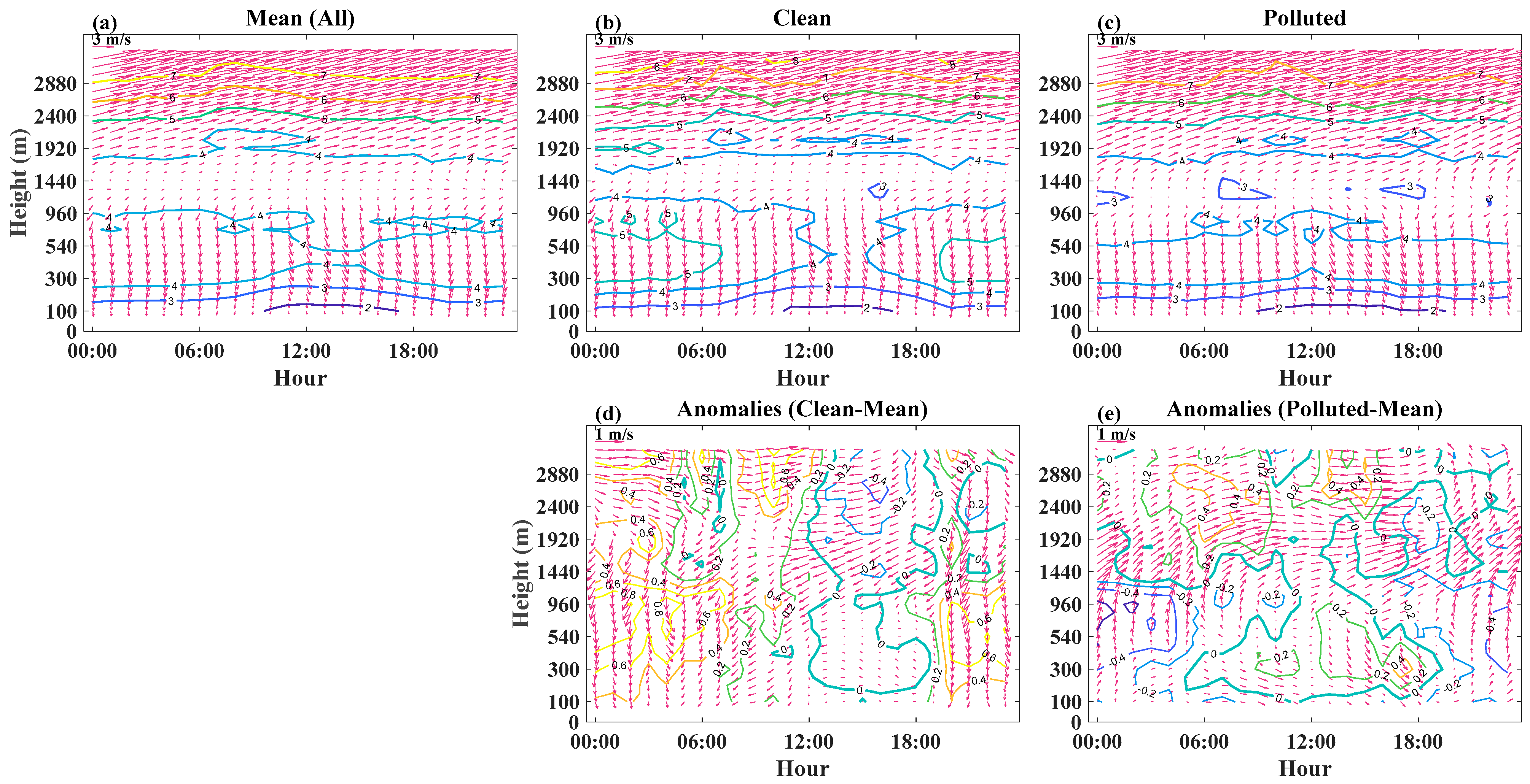
3.2. Diurnal Variations of Vertical Winds

Figure 4 presents the diurnal variations of wind vectors in CS from the surface to 3 km above ground level (km a.g.l., herein km), as well as the anomalies relative to the wintertime averages under mean, polluted, and clean conditions from 2016–2020. The averaged wind speed in the lower troposphere was found to increase with a height from the surface to 0.5 km, referred to be the top of ABL, then decreased with a height from 0.5 to 1.5 km, and increased again above 1.5 km (Figure 4a–c). The wind vector changed from northwest to northeast between ground and 1 km and veered to southwest above 1.5 km (Figure 4a). Changing wind directions in the lowest layers might be induced by friction-related processes, while the above backing winds were the indication of cold advection [32,69].
For clean conditions, the wind speed dramatically reduced in the afternoon (12:00–18:00 LST), and the northerly anomalies enhanced in the nighttime and morning throughout the altitude from the surface up to 2 km (Figure 4b,d), which was consistent with the variations of surface wind speed. For polluted conditions, the wind speed enhanced slightly during the daytime (Figure 4c,e). The weakened wind speed of around 1 km stabilized the lower stratifications, and the simultaneous increasing wind speed at 300 m might cause small turbulence intensity in ABL, unfavorable for the diffusion of near-surface PM2.5 [65,66].
Due to the limitation of observation data from RWP in JM, we focused on the wind profiles below 1 km, mainly covering ABL height (Figure 5). The lower troposphere was controlled by the northeast wind with peaking wind speed at 06:00 LST, and the peak extended to 10:00 LST for clean conditions. The enhanced southerly wind anomalies at 06:00 and 17:00 LST weakened the wind speed and shifted the wind direction to easterly in the afternoon under clean conditions, which diminished the vertical gradients of wind. In contrast, the positive wind speed anomalies overlaid the peak values of wind speed at 06:00 LST, thus enhancing the vertical gradients of wind speed under polluted conditions, which is different from the stable condition with the weak wind in CS. The unique distribution of diurnal cycles in wind and wind anomalies in JM might be influenced by the local circulation induced by terrain [37], identifying the noteworthy regional feature in the northern THB.

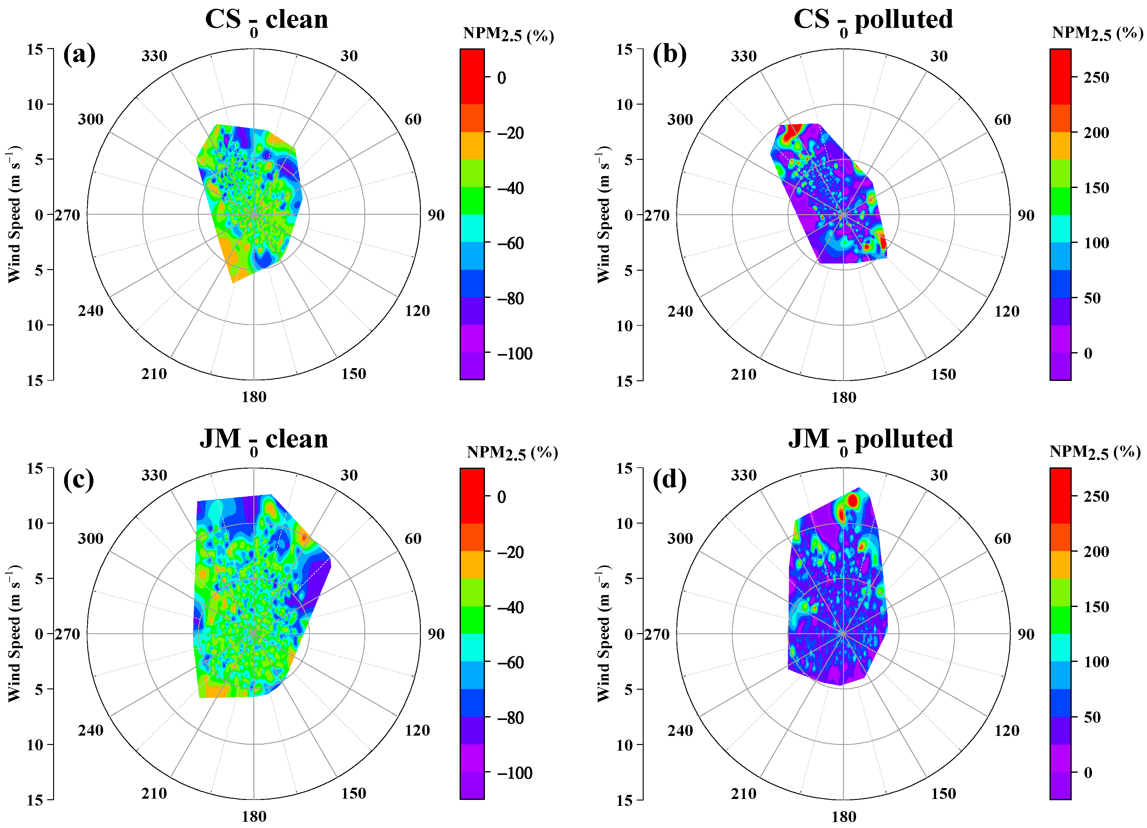
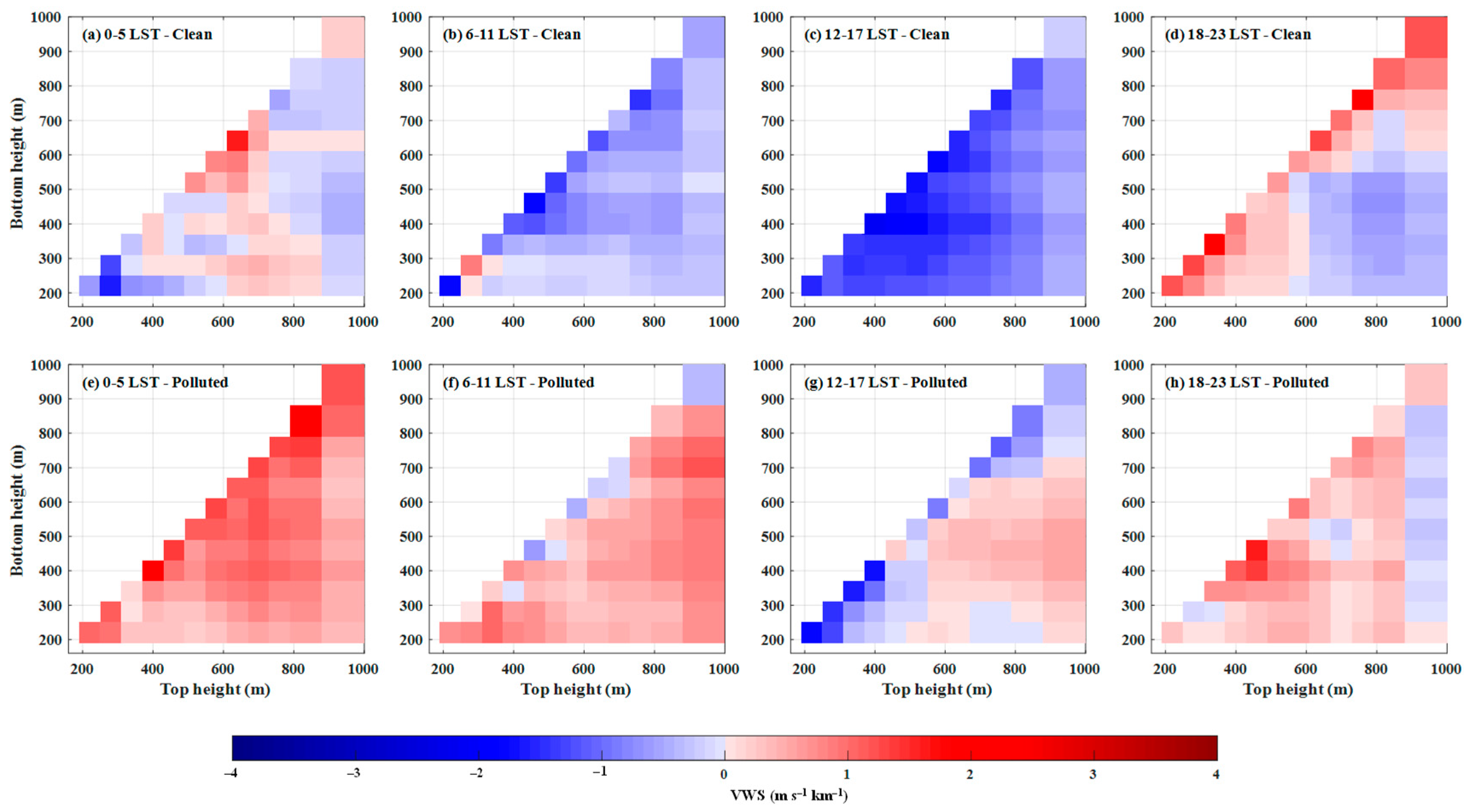
3.3. Effect of Vertical Wind Shear on PM2.5 Concentration

VWS significantly impacts the vertical mixing of air pollutants in ABL and leads to changes in near-surface air pollutants [28]. Hence, we further distinguished the vertical distribution of VWS intensity under clean and polluted conditions. Generally, the patterns of VWS were consistent from clean to polluted conditions with the highest values between the two nearest layers (Figures S4 and S5).
For both polluted and clean conditions in CS, the strongest VWS occurred near the surface with several peak values distributed at higher altitudes. The high surface values resulted from the friction-related processes, and the upper peak values might be induced by the low-level jet or advection associated with the synoptic process [21,70]. On average, the VWS magnitude in polluted conditions was found to be smaller than in clean conditions in CS, especially in the layer above 1.5 km, revealing the more significant contribution of turbulent mixing aloft than near the surface in clean conditions (Figure S4). The positive anomalies of VWS were concentrated in the upper layers under clean conditions and turned to near-surface under polluted conditions (Figure 6). For clean conditions, the VWS anomalies were generally positive with negative anomalies existing in the daytime below 1.5 km, which resulted from the weakened wind speed (Figure 4d and Figure 6a–d). Most of the VWS anomalies in the lower layers were positive for polluted conditions, although the wind speed anomalies were negative at night (Figure 4e and Figure 6e–h).
To further figure out the association between VWS and surface PM2.5, we presented the distribution of correlation coefficients between NPM2.5 and VWS in CS, exhibiting contrast features under clean and polluted conditions in the lower troposphere (Figure 7). For clean conditions, the correlation coefficients between VWS and NPM2.5 were ubiquitously negative from ground level up to 3 km, revealing that the increase in VWS accompanied by enhanced vertical mixing led to the dispersion of PM2.5 near the surface (Figure 7a). Meanwhile, the distribution of correlation coefficients between VWS and NPM2.5 for polluted conditions presented a “sandwich” pattern of positive near the surface, negative at altitudes of 1–2 km, and positive above 2 km. The positive correlation coefficients from the surface up to 1 km revealed the increasing VWS under weak wind conditions in ABL, favoring the PM2.5 increase. The correlation coefficients shifting from positive to negative at altitudes of 1–2 km suggested that the stronger VWS above ABL was associated with lower surface PM2.5 concentrations. The positive values at heights above 2 km might be linked to the regional transport of air pollutants, revealing a transport height of above 2 km in CS [71].
The magnitude of VWS below 1 km in JM was higher than that in CS, and the VWS was stronger under polluted conditions than under clean conditions, differing from the features in CS (Figures S4 and S5). Meanwhile, the nocturnal VWS increased more markedly than in the daytime under both clean and polluted conditions. The positive anomalies were scattered at night for clean conditions but had higher impact during the whole day for polluted conditions (Figure 8). The diurnal variations of VWS anomalies were not consistent with wind speed anomalies, and the correlation coefficients of VWS and NPM2.5 were positive during clean and polluted conditions in JM. The high correlation coefficients under clean conditions were near the surface but were elevated to a height of ~500–800 m under polluted conditions (Figure 9). The peaks of wind speed near the surface overlaid with negative wind speed anomalies led to the weakened vertical gradient of wind speed and decreased VWS for clean conditions (Figure 5), leading to uniformly distributed winds and facilitating the horizontal diffusion of air pollutants, causing the positive correlation between VWS and PM2.5 for clean conditions. However, the positive anomalies of wind speed occurred in weak wind zones; thus, the vertical gradient became larger, leading to stronger VWS for polluted conditions. The increased VWS with strong wind enhanced vertical mixing, which blocked the air pollutants in the local region and might bring in the transported air pollutants from upstream regions in the upper layers.
Based on the analysis above, there was a distinct impact of VWS on surface PM2.5 concentrations in downstream CS and upstream JM, which seemed not to be caused by the variation in synoptic weather, indicating the non-negligible effect of local circulation on ABL structure. The influence of regional transport induced by prevailing northerly winds on the VWS structure was more significant in upstream JM, attenuating the difference between clean and pollution conditions.

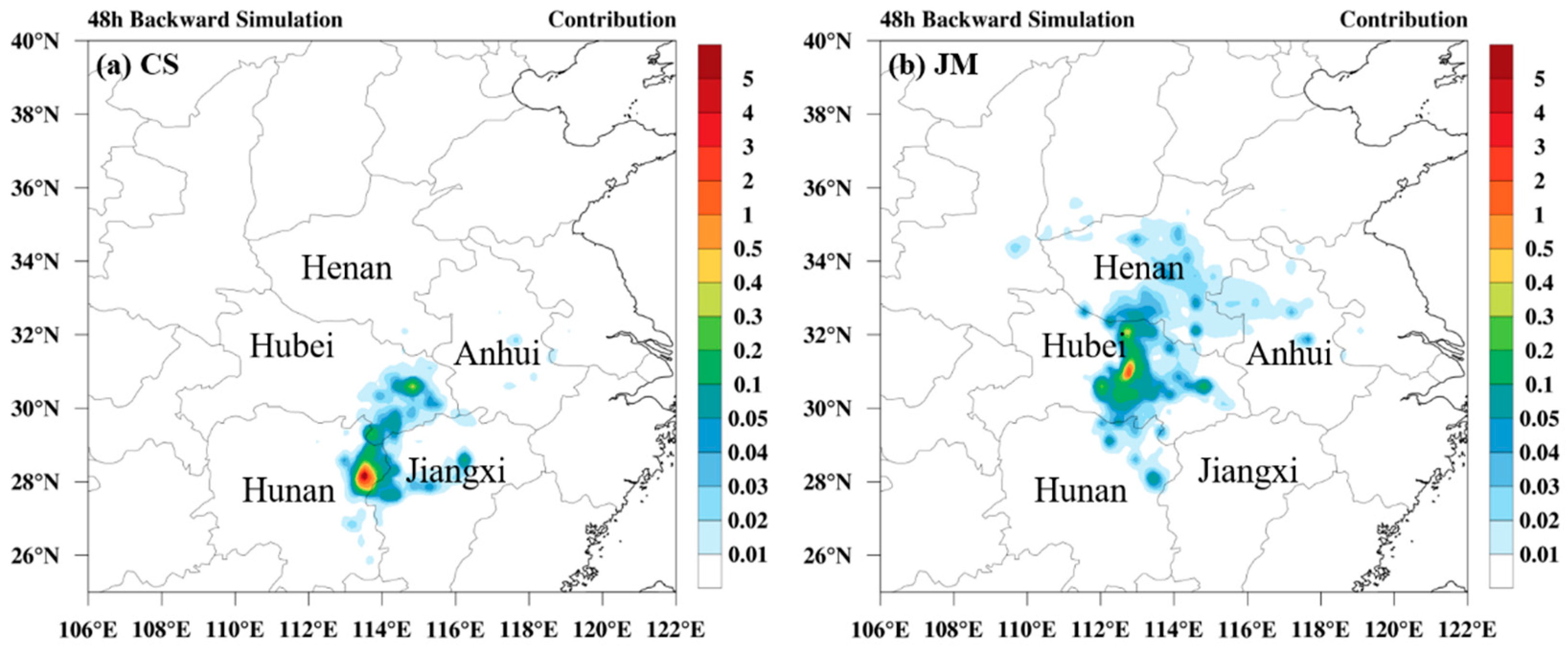
3.4. Backward Trajectory Modeling Analysis

The above observational study investigated the different impacts of regional transport on the vertical structure of VWS in the upstream and downstream sites of the receptor region in central China. To further quantify the contribution of regional transport to PM2.5 pollution in this receptor region, backward trajectory modeling using WRF-FLEXPART was conducted to identify the backward trajectory of PM2.5 and to estimate the resulting contributions [39]. Governed by the wintertime prevailing north winds, central China to the north of THB was recognized as a key emission source region for PM2.5 pollution in THB, illustrated in the potential contribution source maps (Figure 10). The PM2.5 pollution in CS was mainly sourced from local emissions and the adjacent megacities, but the influence domain of regional transport in JM was broader, extending to northern China.
We listed the contribution rates of provinces in central China to PM2.5 concentrations in receptors in Table 3. We take Hubei and Hunan provinces as the local regions for JM and CS, respectively. Hubei province in the north and Jiangxi province in the east were the main external source regions for regional transport of PM2.5 to CS, and Henan province in the north was the most important external source for regional transport to JM, driven by prevailed northerly and northeasterly winds of East Asian winter monsoons. The contribution of THB (approximately considered as Hubei and Hunan provinces) to PM2.5 in CS was 81.9%, while the contribution was down to 57.7% in JM, indicating the more important role of regional PM2.5 transport on surface PM2.5 concentrations in upstream JM than that in downstream CS.

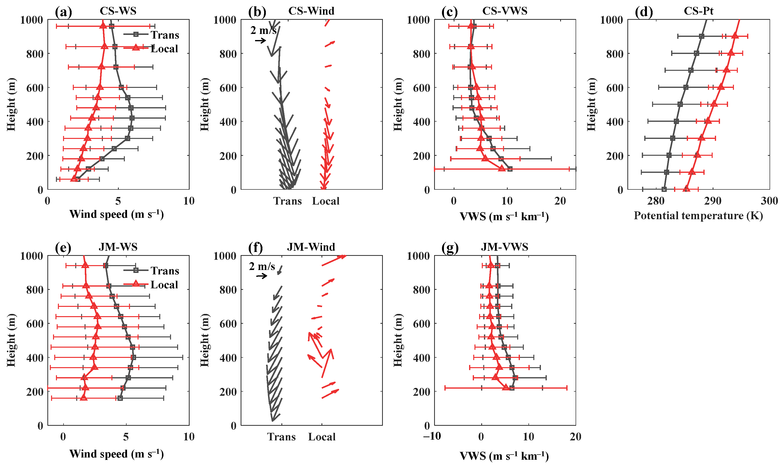
3.5. Causes for Transport- and Local-Type PM2.5 Pollution

To inquire into the impact of regional transport on ABL structures, we select five typical regional transport-inducing (transport-type) pollution days and five typical local accumulation-inducing (local-type) pollution days of regional PM2.5 pollution (both the daily PM2.5 concentrations in CS and JM > 75 μg m–3) according to the previous studies over THB [37,72]. The average daily PM2.5 concentrations were larger in CS for local-type pollution days, but the pollution was heavier in JM for transport-type pollution days (Table 4), indicating the more significant influence of regional PM2.5 transport on air pollution in JM.
The ensemble vertical profiles of wind and potential temperature for transport-type and local-type pollution days are shown in Figure 11. When regional transport of air pollutants occupied THB, the consistent northerly winds were throughout the layer below 1 km in upstream and downstream sites. Both the wind profiles in CS and JM had a peak at the height of ~400 m during transport-type pollution days, indicating a transport height of ~400 m over THB. VWS below the transport height of 400 m was larger on transport-type pollution days than that on local-type pollution days in CS, and the larger wind speed and VWS in JM on transport-type pollution days extended up to 1 km, confirming the deeper influence of regional transport at upstream site. By comparing the vertical changes of potential temperature in CS, the ABL was more stable on the local-type pollution days. Overall, the regional transport of air pollutants driven by northerly winds strengthened the VWS near the ground and weakened the ABL stability, thus enhancing the vertical mixing of air pollutants, favoring the transported air pollutants down-mixed to the near surface.

4. Conclusions

Based on the high temporal and spatial observation data from RWPs for winters from 2016–2020, we explored the impact of VWS on surface PM2.5 concentrations in two urban cities CS and JM, the upstream and downstream regions along the transport pathway of regional transport in central China. In addition, we conducted WRF-FLEXPART simulations to quantify the contribution of regional PM2.5 transport from source regions to surface PM2.5 concentrations over the receptor region.
With higher anthropogenic PM2.5 emissions, the surface PM2.5 concentrations were lower in CS compared with that in JM, identifying the importance of local meteorological conditions on PM2.5 changes. The weakened wind speed near the surface and decreased VWS in the height of 1–2 km stabilized the ABL structure and resulted in PM2.5 accumulation near the surface under polluted conditions in CS. At the height above 2 km, strong northerlies wind with enhanced VWS also favored the long-range transport of air pollutants, which also deteriorated the air quality in CS. The local circulation induced by the terrain and long-range transport synergistically led to the different diurnal variations of wind and VWS in JM from that in CS. The VWS was positively correlated with surface PM2.5 concentrations under clean and polluted conditions in JM, suggesting the unique VWS structure and more significant influence of regional transport in the upstream region, which was confirmed with the simulation results using WRF-FLEXPART. The strong northerly wind distributed evenly in the lower troposphere with stronger wind speed and VWS under transport-type polluted conditions, in sharp contrast to the weak wind under local-type polluted conditions, which also suggested the more significant response of ABL structures in JM to regional transport. The non-stagnant conditions during transport-type pollution days facilitated our understanding of the regional transport in air quality changes.
This study revealed the different VWS characteristics for heavy air pollution with regional PM2.5 transport based on the changes in PM2.5 and meteorology in two sites over a receptor region. Due to the data quality of RWPs, there is a lack of VWS in the layers above 1 km in JM. The effect of ABL structures on air pollution can be further explored with multi-source satellite data and long-term lidar observation. The simulation using FLEXPART is also sensitive to release data, such as release height, and species composition, which are approximated in the present simulation in the absence of relevant data [48], leading the limitations for the characterization of the potential sources in the current study. A comprehensive model simulation of air quality and meteorology with refined physical and chemical schemes and data assimilation in ABL is desired in further studies.

Supplementary Materials

The following supporting information can be downloaded at: https://www.mdpi.com/article/10.3390/rs14143333/s1, Figure S1: Time-height cross-sections of horizontal wind speed (color shaded) from RWP in (a) CS and (b) JM, overlaid with observed surface PM2.5 concentrations (black lines) for winters over 2016–2020; Figure S2: Two nesting domains d01 and d02 for the WRF simulation; Figure S3: The spatial distribution of PM2.5 emissions (mainly in the transportation, agriculture, industry, power and residual sectors) during winter in 2016, as acquired from the multi-resolution emission inventory for China (MEIC); Figure S4: 6-hourly averaged VWS computed between different heights under (a–d) clean and (e–h) polluted conditions in CS for (a,e) 00:00–05:00 LST, (b,f) 06:00–11:00 LST, (c,g) 12:00–17:00 LST, and (d,h) 18:00–23:00 LST, during the period of winters over 2016–2020; Figure S5: 6-hourly averaged VWS computed between different heights under (a–d) clean and (e–h) polluted conditions in JM for (a,e) 00:00–05:00 LST, (b,f) 06:00–11:00 LST, (c,g) 12:00–17:00 LST, and (d,h) 18:00–23:00 LST, during the period of winters over 2016–2020; Table S1: Evaluation results for the modeling meteorological parameters with the observations in winter over 2016–2020. Obs. is mean observation; Sim. is mean simulation; r is correlation coefficient; RMSE is root mean square error; MFB is the mean fractional bias; MFE is the mean fractional error.

Author Contributions

Conceptualization, X.S. and Y.Z.; Resources, T.H. and H.H.; Data curation, L.L. and J.S.; methodology, X.S.; investigation, Y.Z., Y.B. and T.Z.; writing—original draft preparation, X.S.; writing—review and editing, X.S. and Y.Z.; funding acquisition, T.Z. All authors have read and agreed to the published version of the manuscript.

Funding

This research was funded by the National Natural Science Foundation of China, grant numbers 41830965, 41875170, 42075186 and 91744209.

Data Availability Statement

Data used in this paper can be provided by Xiaoyun Sun ([email protected]) upon request.

Acknowledgments

We are grateful to Changsha Meteorological Bureau and Jingmen Meteorological Bureau for providing the wind profile data used in this study.

Conflicts of Interest

The authors declare no conflict of interest.

References

  1. Peng, J.; Chen, S.; Lü, H.L.; Liu, Y.X.; Wu, J.S. Spatiotemporal patterns of remotely sensed PM 2.5 concentration in China from 1999 to 2011. Remote Sens. Environ. 2016, 174, 109–121. [Google Scholar] [CrossRef]
  2. Wang, X.Y.; Wang, K.C.; Su, L.Y. Contribution of atmospheric diffusion conditions to the recent improvement in air quality in China. Sci. Rep. 2016, 6, 36404. [Google Scholar] [CrossRef] [PubMed] [Green Version]
  3. Cao, J.J.; Wang, Q.Y.; Chow, J.C.; Watson, J.G.; Tie, X.X.; Shen, Z.X.; Wang, P.; An, Z.S. Impacts of aerosol compositions on visibility impairment in Xi’an, China. Atmos. Environ. 2012, 59, 559–566. [Google Scholar] [CrossRef]
  4. Crouse, D.L.; Peters, P.A.; van Donkelaar, A.; Goldberg, M.S.; Villeneuve, P.J.; Brion, O.; Khan, S.; Atari, D.O.; Jerrett, M.; Pope III, C.A. Risk of nonaccidental and cardiovascular mortality in relation to long-term exposure to low concentrations of fine particulate matter: A Canadian national-level cohort study. Environ. Health Perspect. 2012, 120, 708–714. [Google Scholar] [CrossRef]
  5. Zhang, X.Y.; Xu, X.D.; Ding, Y.H.; Liu, Y.J.; Zhang, H.D.; Wang, Y.Q.; Zhong, J.T. The impact of meteorological changes from 2013 to 2017 on PM 2.5 mass reduction in key regions in China. Sci. China Earth Sci. 2019, 62, 1885–1902. [Google Scholar] [CrossRef]
  6. Xiao, Q.; Zheng, Y.; Geng, G.; Chen, C.; Huang, X.; Che, H.; Zhang, X.; He, K.; Zhang, Q. Separating emission and meteorological contributions to long-term PM2.5 trends over eastern China during 2000–2018. Atmos. Chem. Phys. 2021, 21, 9475–9496. [Google Scholar] [CrossRef]
  7. Gong, S.L.; Liu, H.L.; Zhang, B.H.; He, J.J.; Zhang, H.D.; Wang, Y.Q.; Wang, S.X.; Zhang, L.; Wang, J. Assessment of meteorology vs. control measures in the China fine particular matter trend from 2013 to 2019 by an environmental meteorology index. Atmos. Chem. Phys. 2021, 21, 2999–3013. [Google Scholar] [CrossRef]
  8. Zheng, B.; Tong, D.; Li, M.; Liu, F.; Hong, C.P.; Geng, G.N.; Li, H.Y.; Li, X.; Peng, L.Q.; Qi, J. Trends in China’s anthropogenic emissions since 2010 as the consequence of clean air actions. Atmos. Chem. Phys. 2018, 18, 14095–14111. [Google Scholar] [CrossRef] [Green Version]
  9. Zhang, Q.; Ma, Q.; Zhao, B.; Liu, X.; Wang, Y.; Jia, B.; Zhang, X. Winter haze over North China Plain from 2009 to 2016: Influence of emission and meteorology. Environ. Pollut. 2018, 242, 1308–1318. [Google Scholar] [CrossRef]
  10. Huang, X.; Ding, A.; Wang, Z.; Ding, K.; Gao, J.; Chai, F.; Fu, C. Amplified transboundary transport of haze by aerosol–boundary layer interaction in China. Nat. Geosci. 2020, 13, 428–434. [Google Scholar] [CrossRef]
  11. Cai, W.; Li, K.; Liao, H.; Wang, H.; Wu, L. Weather conditions conducive to Beijing severe haze more frequent under climate change. Nat. Clim. Chang. 2017, 7, 257–262. [Google Scholar] [CrossRef]
  12. Zou, Y.; Wang, Y.; Zhang, Y.; Koo, J.-H. Arctic sea ice, Eurasia snow, and extreme winter haze in China. Sci. Adv. 2017, 3, e1602751. [Google Scholar] [CrossRef] [PubMed] [Green Version]
  13. Lu, M.M.; Tang, X.; Wang, Z.F.; Gbaguidi, A.; Liang, S.W.; Hu, K.; Wu, L.; Wu, H.J.; Huang, Z.; Shen, L.J. Source tagging modeling study of heavy haze episodes under complex regional transport processes over Wuhan megacity, Central China. Environ. Pollut. 2017, 231, 612–621. [Google Scholar] [CrossRef] [PubMed]
  14. Li, K.; Liao, H.; Cai, W.J.; Yang, Y. Attribution of anthropogenic influence on atmospheric patterns conducive to recent most severe haze over eastern China. Geophys. Res. Lett. 2018, 45, 2072–2081. [Google Scholar] [CrossRef]
  15. Bai, K.; Li, K.; Guo, J.; Cheng, W.; Xu, X. Do More Frequent Temperature Inversions Aggravate Haze Pollution in China? Geophys. Res. Lett. 2022, 49, e2021GL096458. [Google Scholar] [CrossRef]
  16. Ding, A.; Huang, X.; Nie, W.; Sun, J.; Kerminen, V.M.; Petäjä, T.; Su, H.; Cheng, Y.; Yang, X.Q.; Wang, M. Enhanced haze pollution by black carbon in megacities in China. Geophys. Res. Lett. 2016, 43, 2873–2879. [Google Scholar] [CrossRef]
  17. Huang, X.; Wang, Z.; Ding, A. Impact of aerosol-PBL interaction on haze pollution: Multiyear observational evidences in North China. Geophys. Res. Lett. 2018, 45, 8596–8603. [Google Scholar] [CrossRef] [Green Version]
  18. Dong, Z.; Li, Z.; Yu, X.; Cribb, M.; Li, X.; Dai, J. Opposite long-term trends in aerosols between low and high altitudes: A testimony to the aerosol–PBL feedback. Atmos. Chem. Phys. 2017, 17, 7997–8009. [Google Scholar] [CrossRef] [Green Version]
  19. Li, Z.; Guo, J.; Ding, A.; Liao, H.; Liu, J.; Sun, Y.; Wang, T.; Xue, H.; Zhang, H.; Zhu, B. Aerosol and boundary-layer interactions and impact on air quality. Natl. Sci. Rev. 2017, 4, 810–833. [Google Scholar] [CrossRef]
  20. Zheng, G.; Duan, F.; Su, H.; Ma, Y.; Cheng, Y.; Zheng, B.; Zhang, Q.; Huang, T.; Kimoto, T.; Chang, D. Exploring the severe winter haze in Beijing: The impact of synoptic weather, regional transport and heterogeneous reactions. Atmos. Chem. Phys. 2015, 15, 2969–2983. [Google Scholar] [CrossRef] [Green Version]
  21. Li, X.; Hu, X.-M.; Ma, Y.; Wang, Y.; Li, L.; Zhao, Z. Impact of planetary boundary layer structure on the formation and evolution of air-pollution episodes in Shenyang, Northeast China. Atmos. Environ. 2019, 214, 116850. [Google Scholar] [CrossRef]
  22. Zhang, K.; Wang, D.; Bian, Q.; Duan, Y.; Zhao, M.; Fei, D.; Xiu, G.; Fu, Q. Tethered balloon-based particle number concentration, and size distribution vertical profiles within the lower troposphere of Shanghai. Atmos. Environ. 2017, 154, 141–150. [Google Scholar] [CrossRef]
  23. Dolman, B.K.; Reid, I.M.; Tingwell, C. Stratospheric tropospheric wind profiling radars in the Australian network. Earth Planets Space 2018, 70, 170. [Google Scholar] [CrossRef] [Green Version]
  24. Molod, A.; Salmun, H.; Dempsey, M. Estimating planetary boundary layer heights from NOAA profiler network wind profiler data. J. Atmos. Ocean. Technol. 2015, 32, 1545–1561. [Google Scholar] [CrossRef]
  25. Ishihara, M.; Kato, Y.; Abo, T.; Kobayashi, K.; Izumikawa, Y. Characteristics and performance of the operational wind profiler network of the Japan Meteorological Agency. J. Meteorol. Soc. Jpn. Ser. II 2006, 84, 1085–1096. [Google Scholar] [CrossRef] [Green Version]
  26. Harvey, N.J.; Hogan, R.J.; Dacre, H.F. A method to diagnose boundary-layer type using Doppler lidar. Q. J. R. Meteorol. Soc. 2013, 139, 1681–1693. [Google Scholar] [CrossRef]
  27. Manninen, A.; Marke, T.; Tuononen, M.; O’Connor, E. Atmospheric boundary layer classification with Doppler lidar. J. Geophys. Res. Atmos. 2018, 123, 8172–8189. [Google Scholar] [CrossRef]
  28. Yang, Y.; Yim, S.H.; Haywood, J.; Osborne, M.; Chan, J.C.; Zeng, Z.; Cheng, J.C. Characteristics of heavy particulate matter pollution events over Hong Kong and their relationships with vertical wind profiles using high-time-resolution Doppler lidar measurements. J. Geophys. Res. Atmos. 2019, 124, 9609–9623. [Google Scholar] [CrossRef] [Green Version]
  29. Sekuła, P.; Bokwa, A.; Bartyzel, J.; Bochenek, B.; Chmura, Ł.; Gałkowski, M.; Zimnoch, M. Measurement report: Effect of wind shear on PM10 concentration vertical structure in the urban boundary layer in a complex terrain. Atmos. Chem. Phys. 2021, 21, 12113–12139. [Google Scholar] [CrossRef]
  30. Tie, X.; Zhang, Q.; He, H.; Cao, J.; Han, S.; Gao, Y.; Li, X.; Jia, X.C. A budget analysis of the formation of haze in Beijing. Atmos. Environ. 2015, 100, 25–36. [Google Scholar] [CrossRef]
  31. Liu, B.; Guo, J.; Gong, W.; Shi, L.; Zhang, Y.; Ma, Y. Characteristics and performance of wind profiles as observed by the radar wind profiler network of China. Atmos. Meas. Tech. 2020, 13, 4589–4600. [Google Scholar] [CrossRef]
  32. Zhang, Y.; Guo, J.; Yang, Y.; Wang, Y.; Yim, S.H. Vertical wind shear modulates particulate matter pollutions: A perspective from Radar wind profiler observations in Beijing, China. Remote Sens. 2020, 12, 546. [Google Scholar] [CrossRef] [Green Version]
  33. Huang, T.; Yim, S.H.-l.; Yang, Y.; Lee, O.S.-m.; Lam, D.H.-y.; Cheng, J.C.-h.; Guo, J. Observation of turbulent mixing characteristics in the typical daytime cloud-topped boundary layer over Hong Kong in 2019. Remote Sens. 2020, 12, 1533. [Google Scholar] [CrossRef]
  34. Shen, L.J.; Wang, H.L.; Zhao, T.L.; Liu, J.; Bai, Y.Q.; Kong, S.F.; Shu, Z.Z. Characterizing regional aerosol pollution in central China based on 19 years of MODIS data: Spatiotemporal variation and aerosol type discrimination. Environ. Pollut. 2020, 263, 114556. [Google Scholar] [CrossRef]
  35. Tan, C.; Zhao, T.; Xu, X.; Liu, J.; Zhang, L.; Tang, L. Climatic analysis of satellite aerosol data on variations of submicron aerosols over East China. Atmos. Environ. 2015, 123, 392–398. [Google Scholar] [CrossRef]
  36. Lin, C.Q.; Liu, G.H.; Lau, A.K.H.; Li, Y.; Li, C.C.; Fung, J.C.H.; Lao, X.Q. High-resolution satellite remote sensing of provincial PM2. 5 trends in China from 2001 to 2015. Atmos. Environ. 2018, 180, 110–116. [Google Scholar] [CrossRef]
  37. Bai, Y.; Zhao, T.; Hu, W.; Zhou, Y.; Xiong, J.; Wang, Y.; Liu, L.; Shen, L.; Kong, S.; Meng, K.; et al. Meteorological mechanism of regional PM2.5 transport building a receptor region for heavy air pollution over Central China. Sci. Total Environ. 2022, 808, 151951. [Google Scholar] [CrossRef]
  38. Zhong, J.T.; Zhang, X.Y.; Wang, Y.Q.; Wang, J.Z.; Shen, X.J.; Zhang, H.S.; Wang, T.J.; Xie, Z.Q.; Liu, C.; Zhang, H.D. The two-way feedback mechanism between unfavorable meteorological conditions and cumulative aerosol pollution in various haze regions of China. Atmos. Chem. Phys. 2019, 19, 3287–3306. [Google Scholar] [CrossRef] [Green Version]
  39. Yu, C.; Zhao, T.L.; Bai, Y.Q.; Zhang, L.; Kong, S.F.; Yu, X.N.; He, J.H.; Cui, C.G.; Yang, J.; You, Y.C. Heavy air pollution with a unique “non-stagnant” atmospheric boundary layer in the Yangtze River middle basin aggravated by regional transport of PM 2.5 over China. Atmos. Chem. Phys. 2020, 20, 7217–7230. [Google Scholar] [CrossRef]
  40. Sun, X.; Zhao, T.; Bai, Y.; Kong, S.; Zheng, H.; Hu, W.; Ma, X.; Xiong, J. Meteorology impact on PM 2.5 change over a receptor region in the regional transport of air pollutants: Observational study of recent emission reductions in central China. Atmos. Chem. Phys. 2022, 22, 3579–3593. [Google Scholar] [CrossRef]
  41. Ministry of Ecology and Environment of the People’s Republic of China. Available online: http://www.mee.gov.cn/ (accessed on 24 June 2022).
  42. China Meteorological Data Service Center. Available online: http://data.cma.cn/ (accessed on 24 June 2022).
  43. Miao, Y.; Guo, J.; Liu, S.; Wei, W.; Zhang, G.; Lin, Y.; Zhai, P. The climatology of low-level jet in Beijing and Guangzhou, China. J. Geophys. Res. Atmos. 2018, 123, 2816–2830. [Google Scholar] [CrossRef]
  44. Guo, J.; Deng, M.; Fan, J.; Li, Z.; Chen, Q.; Zhai, P.; Dai, Z.; Li, X. Precipitation and air pollution at mountain and plain stations in northern China: Insights gained from observations and modeling. J. Geophys. Res. Atmos. 2014, 119, 4793–4807. [Google Scholar] [CrossRef]
  45. Wang, X.; Dickinson, R.E.; Su, L.; Zhou, C.; Wang, K. PM2. 5 pollution in China and how it has been exacerbated by terrain and meteorological conditions. Bull. Am. Meteorol. Soc. 2018, 99, 105–119. [Google Scholar] [CrossRef]
  46. Markowski, P.; Richardson, Y. On the classification of vertical wind shear as directional shear versus speed shear. Weather Forecast. 2006, 21, 242–247. [Google Scholar] [CrossRef] [Green Version]
  47. Brioude, J.; Arnold, D.; Stohl, A.; Cassiani, M.; Morton, D.; Seibert, P.; Angevine, W.; Evan, S.; Dingwell, A.; Fast, J.D. The Lagrangian particle dispersion model FLEXPART-WRF version 3.1. Geosci. Model. Dev. 2013, 6, 1889–1904. [Google Scholar] [CrossRef] [Green Version]
  48. Karmakar, S.; Srinivas, C.; Rakesh, P.; Venkatesan, R.; Venkatraman, B. A WRF-FLEXPART simulation study of oil-fire plume dispersion-sensitivity to turbulent diffusion schemes. Meteorol. Atmos. Phys. 2022, 134, 32. [Google Scholar] [CrossRef]
  49. Grell, G.A.; Peckham, S.E.; Schmitz, R.; McKeen, S.A.; Frost, G.; Skamarock, W.C.; Eder, B. Fully coupled “online” chemistry within the WRF model. Atmos. Environ. 2005, 39, 6957–6975. [Google Scholar] [CrossRef]
  50. Hong, S.Y.; Noh, Y. A New Vertical Diffusion Package with an Explicit Treatment of Entrainment Processes. Mon. Weather Rev. 2006, 134, 2318–2341. [Google Scholar] [CrossRef] [Green Version]
  51. Mlawer, E.J.; Taubman, S.J.; Brown, P.D.; Iacono, M.J.; Clough, S.A. Radiative transfer for inhomogeneous atmospheres: RRTM, a validated correlated-k model for the longwave. J. Geophys. Res. Atmos. 1997, 102, 16663–16682. [Google Scholar] [CrossRef] [Green Version]
  52. Chou, M.D.; Suarez, M.J. Parameterizations for Cloud Overlapping and Shortwave Single-Scattering. J. Clim. 1998, 11, 202–214. [Google Scholar] [CrossRef]
  53. Lin, Y.L.; Farley, R.D.; Orville, H.D. Bulk Parameterization of the Snow Field in a Cloud Model. J. Clim. Appl. Meteorol. 1983, 22, 1065–1092. [Google Scholar] [CrossRef] [Green Version]
  54. National Centers for Environmental Prediction; NWS; NOAA; U.S. Department of Commerce. NCEP FNL Operational Model Global Tropospheric Analyses, Continuing from July 1999. Available online: https://doi.org/10.5065/D6M043C6 (accessed on 24 June 2022).
  55. Boylan, J.W.; Russell, A.G. PM and light extinction model performance metrics, goals, and criteria for three-dimensional air quality models. Atmos. Environ. 2006, 40, 4946–4959. [Google Scholar] [CrossRef]
  56. Morris, R.E.; McNally, D.E.; Tesche, T.W.; Tonnesen, G.; Boylan, J.W.; Brewer, P. Preliminary evaluation of the Community Multiscale Air Quality model for 2002 over the southeastern United States. J. Air Waste Manag. Assoc. 2005, 55, 1694–1708. [Google Scholar] [CrossRef] [PubMed]
  57. Stohl, A.; Forster, C.; Eckhardt, S.; Spichtinger, N.; Huntrieser, H.; Heland, J.; Schlager, H.; Wilhelm, S.; Arnold, F.; Cooper, O. A backward modeling study of intercontinental pollution transport using aircraft measurements. J. Geophys. Res. Atmos. 2003, 108, 4370. [Google Scholar] [CrossRef]
  58. Stohl, A.; Forster, C.; Frank, A.; Seibert, P.; Wotawa, G. The Lagrangian particle dispersion model FLEXPART version 6.2. Atmos. Chem. Phys. 2005, 5, 2461–2474. [Google Scholar] [CrossRef] [Green Version]
  59. Ding, A.; Wang, T.; Xue, L.; Gao, J.; Stohl, A.; Lei, H.; Jin, D.; Ren, Y.; Wang, X.; Wei, X. Transport of north China air pollution by midlatitude cyclones: Case study of aircraft measurements in summer 2007. J. Geophys. Res. Atmos. 2009, 114, D08304. [Google Scholar] [CrossRef] [Green Version]
  60. Multi-Resolution Emission Inventory for China. Available online: http://meicmodel.org (accessed on 24 June 2022).
  61. Yu, R.; Li, J.; Chen, H. Diurnal variation of surface wind over central eastern China. Clim. Dyn. 2009, 33, 1089–1097. [Google Scholar] [CrossRef]
  62. Wang, H.; Li, Z.; Lv, Y.; Zhang, Y.; Xu, H.; Guo, J.; Goloub, P. Determination and climatology of the diurnal cycle of the atmospheric mixing layer height over Beijing 2013–2018: Lidar measurements and implications for air pollution. Atmos. Chem. Phys. 2020, 20, 8839–8854. [Google Scholar] [CrossRef]
  63. He, J.; Gong, S.; Yu, Y.; Yu, L.; Wu, L.; Mao, H.; Song, C.; Zhao, S.; Liu, H.; Li, X. Air pollution characteristics and their relation to meteorological conditions during 2014–2015 in major Chinese cities. Environ. Pollut. 2017, 223, 484–496. [Google Scholar] [CrossRef]
  64. Chen, Z.Y.; Chen, D.L.; Zhao, C.F.; Kwan, M.-P.; Cai, J.; Zhuang, Y.; Zhao, B.; Wang, X.Y.; Chen, B.; Yang, J. Influence of meteorological conditions on PM2. 5 concentrations across China: A review of methodology and mechanism. Environ. Int. 2020, 139, 105558. [Google Scholar] [CrossRef]
  65. Ren, J.; Liu, J.; Li, F.; Cao, X.; Ren, S.; Xu, B.; Zhu, Y. A study of ambient fine particles at Tianjin International Airport, China. Sci. Total Environ. 2016, 556, 126–135. [Google Scholar] [CrossRef] [PubMed]
  66. Yang, Q.; Yuan, Q.; Li, T.; Shen, H.; Zhang, L. The relationships between PM2. 5 and meteorological factors in China: Seasonal and regional variations. Int. J. Environ. Res. Public Health 2017, 14, 1510. [Google Scholar] [CrossRef] [PubMed] [Green Version]
  67. Yuan, S.; Xu, W.; Liu, Z. A study on the model for heating influence on PM2. 5 emission in Beijing China. Procedia Eng. 2015, 121, 612–620. [Google Scholar] [CrossRef] [Green Version]
  68. Zhao, D.; Xin, J.; Gong, C.; Quan, J.; Liu, G.; Zhao, W.; Wang, Y.; Liu, Z.; Song, T. The formation mechanism of air pollution episodes in Beijing city: Insights into the measured feedback between aerosol radiative forcing and the atmospheric boundary layer stability. Sci. Total Environ. 2019, 692, 371–381. [Google Scholar] [CrossRef]
  69. Han, S.-q.; Hao, T.-y.; Zhang, Y.-f.; Li, P.-y.; Cai, Z.-y.; Zhang, M.; Wang, Q.-l.; Zhang, H. Vertical observation and analysis on rapid formation and evolutionary mechanisms of a prolonged haze episode over central-eastern China. Sci. Total Environ. 2018, 616, 135–146. [Google Scholar] [CrossRef] [PubMed]
  70. Doswell III, C.A. A review for forecasters on the application of hodographs to forecasting severe thunderstorms. Natl. Weather Dig. 1991, 16, 2–16. [Google Scholar]
  71. Gu, Y.; Yim, S.H.L. The air quality and health impacts of domestic trans-boundary pollution in various regions of China. Environ. Int. 2016, 97, 117–124. [Google Scholar] [CrossRef]
  72. Shen, L.; Hu, W.; Zhao, T.; Bai, Y.; Wang, H.; Kong, S.; Zhu, Y. Changes in the Distribution Pattern of PM 2.5 Pollution over Central China. Remote Sens. 2021, 13, 4855. [Google Scholar] [CrossRef]
Figure 1. The locations of the (a) Twain-Hu basin and (b) monitoring sites in Jingmen and Changsha overlaid with topography (color contour, m a.s.l.). The pink dots, blue pentacles, and black pluse are the locations of PM2.5, radar wind profiler (RWP), and radiosonde (SOND) sites, respectively.
Remotesensing 14 03333 g001
Figure 2. Diurnal cycles of the surface (ac) PM2.5 concentrations and (df) wind field under clean and polluted conditions in CS and JM for winters from 2016–2020. Error bars denote standard deviations.
Remotesensing 14 03333 g002
Figure 3. Bivariate polar plots of hourly variations in wind speed (round radius, m s–1) and direction (angles, °) to normalized PM2.5 concentrations (color contours, μg m–3) in (a,b) CS and (c,d) JM under clean and polluted conditions for winters from 2016–2020.
Remotesensing 14 03333 g003
Figure 4. Diurnal variations of horizontal wind vectors (vectors) and wind speed (colored lines) under (a) climate mean, (b) clean, and (c) polluted conditions, and the anomalies (relative to climate mean) under (d) clean and (e) polluted conditions in CS for winters from 2016–2020.
Remotesensing 14 03333 g004
Figure 5. Diurnal variations of horizontal wind vectors (vectors) and wind speed (colored lines) under (a) climate mean, (b) clean, and (c) polluted conditions, and the anomalies (relative to climate mean) under (d) clean and (e) polluted conditions in JM for winters from 2016–2020.
Remotesensing 14 03333 g005
Figure 6. Anomalies of 6 hourly averaged VWS computed between different heights relative to averages of winters from 2016–2020 under (ad) clean and (eh) polluted conditions in CS for (a,e) 00:00–05:00 LST, (b,f) 06:00–11:00 LST, (c,g) 12:00–17:00 LST, and (d,h) 18:00–23:00 LST.
Remotesensing 14 03333 g006
Figure 7. The distributions of correlation coefficients between NPM2.5 and VWS under (a) clean and (b) polluted conditions in CS. Black dots indicate the Pearson correlation coefficients passing the confidence level of 90%.
Remotesensing 14 03333 g007
Figure 8. Anomalies of 6 hourly averaged VWS computed between different heights relative to averages of winters from 2016–2020 under (ad) clean and (eh) polluted conditions in JM for (a,e) 00:00–05:00 LST, (b,f) 06:00–11:00 LST, (c,g) 12:00–17:00 LST, and (d,h) 18:00–23:00 LST.
Remotesensing 14 03333 g008
Figure 9. The distributions of correlation coefficients between NPM2.5 and VWS under (a) clean and (b) polluted conditions in JM. Black dots indicate the Pearson correlation coefficients passing the confidence level of 90%.
Remotesensing 14 03333 g009
Figure 10. Distributions of contribution rates (units: %) to PM2.5 concentrations in (a) CS and (b) JM for winters from 2016–2020 simulated by the WRF-FLEXPART model.
Remotesensing 14 03333 g010
Figure 11. Vertical profiles of (a,e) wind speed, (b,f) wind, (c,g) VWS, and (d) potential temperature averaged in the transport-type and local-type heavy pollution days in (ad) CS and (eg) JM. Error bars denote the standard deviations.
Remotesensing 14 03333 g011
Table 1. Detailed information on RWPs and radiosonde measurements in CS and JM.
CSJM
RWPCoordinates112.79°E, 28.11°N112.21°E, 30.99°N
VersionsCFL-03CLC-11-D
Vertical levels below 3 km3227
Time resolution6 min6 min
Initial altitude 100 m100 m
Vertical resolution <1 km: 60 m
>1 km: 120 m
<800 m: 60 m
800–1900 m: 120 m
>1900 m: 240 m
ParametersWind speed,
wind direction
Wind speed,
wind direction
RadiosondeCoordinate113.08°E, 28.20°N/
Time resolutionlaunched twice per day
at 08:00 and 20:00 LST
/
ParametersTemperature, pressure, relative humidity/
Table 2. Averaged PM2.5 concentrations and wind speed (expressed as mean ± standard deviation), as well as their correlation coefficients under clean and polluted conditions in JM and CS for winters from 2016–2020.
Averaged PM2.5 Concentrations (μg m–3)Averaged Wind Speed
(m s–3)
Correlation Coefficients
Mean79.82 ± 46.672.84 ± 1.60
CSClean41.77 ± 1.022.96 ± 0.14−0.24 *
Polluted124.89 ± 2.812.90 ± 0.180.16 *
Mean91.28 ± 47.053.63 ± 2.01
JMClean48.24 ± 2.663.86 ± 0.18−0.12 *
Polluted140.11 ± 3.063.58 ± 0.170.11 *
* Passing confidence level of 99%.
Table 3. Contribution rates (%) of main contributing provinces to PM2.5 concentrations in CS and JM for winters from 2016–2020.
HubeiHunanHenanAnhuiJiangxiOthers
CS13.468.50.71.36.59.6
JM50.77.020.85.50.115.9
Table 4. Daily PM2.5 concentrations and wind speed (expressed as mean ± standard deviation) in typical transport-type and local-type heavy PM2.5 pollution days in CS and JM.
Transport-TypeLocal-Type
DateDaily PM2.5 Concentrations
(μg m–3)
DateDaily PM2.5 Concentrations
(μg m–3)
CSJMCSJM
30 January 2017126.67 ± 17.4892.74 ± 68.104 January 2017215.87 ± 13.18165.17 ± 18.89
17 February 2017116.61 ± 89.5592.25 ± 64.515 February 2018121.84 ± 21.54188.76 ± 72.97
4 December 2017118.34 ± 54.10209.72 ± 92.3816 February 2018167.29 ± 33.29149.85 ± 27.76
5 December 2017168.18 ± 56.61175.07 ± 36.671 December 2018263.44 ± 6.05221.30 ± 15.25
29 January 2019147.12 ± 15.21174.20 ± 12.8714 December 2019164.07 ± 22.44153.38 ± 17.95
Average135.38 ± 53.91148.80 ± 91.31 186.50 ± 57.53175.69 ± 67.73
Publisher’s Note: MDPI stays neutral with regard to jurisdictional claims in published maps and institutional affiliations.

