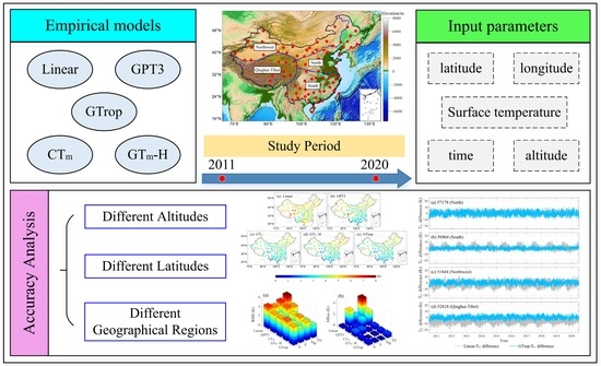
Comprehensive Analysis and Validation of the Atmospheric Weighted Mean Temperature Models in China

Abstract

Atmospheric weighted mean temperature (T_m) is a key parameter used by the Global Navigation Satellite System (GNSS) for calculating precipitable water vapor (PWV). Some empirical T_m models using meteorological or non-meteorological parameters have been proposed to calculate PWV, but their accuracy and reliability cannot be guaranteed in some regions. To validate and determine the optimal T_m model for PWV retrieval in China, this paper analyzes and evaluates some typical T_m models, namely, the Linear, Global Pressure and Temperature 3 (GPT3), the T_m model for China (CT_m), the Global Weighted Mean Temperature-H (GT_m-H) and the Global Tropospheric (GTrop) models. The T_m values of these models are first obtained at corresponding radiosonde (RS) stations in China over the period of 2011 to 2020. The corresponding T_m values of 87 RS stations in China are also calculated using the layered meteorological data and regarded as the reference. Comparison results show that the accuracy of these five T_m models in China has an obvious geographical distribution and decreases along with increasing altitude and latitude, respectively. The average root mean square (RMS) and Bias for the Linear, GPT3, CT_m, GT_m-H and GTrop models are 4.2/3.7/3.4/3.6/3.3 K and 0.7/−1.0/0.7/−0.1/0.3 K, respectively. Among these models, Linear and GPT3 models have lower accuracy in high-altitude regions, whereas CT_m, GT_m-H and GTrop models show better accuracy and stability throughout the whole China. These models generally have higher accuracy in regions with low latitude and lower accuracy in regions with middle and high latitudes. In addition, Linear and GPT3 models have poor accuracy in general, whereas GT_m-H and CT_m models are obviously less accurate and stable than GTrop model in regions with high latitude. These models show different accuracies across the four geographical regions of China, with GTrop model demonstrating the relatively better accuracy and stability. Therefore, the GTrop model is recommended to obtain T_m for calculating PWV in China.

1. Introduction

Atmospheric water vapor is an important greenhouse gas in the atmosphere that plays an important role in climate change and weather forecasting [1]. Therefore, monitoring water vapor with high precision is critical for related studies. The Global Navigation Satellite System (GNSS) receiver can provide continuous and accurate values of precipitable water vapor (PWV) in the zenithal direction over a GNSS station, consequently the high temporal and spatial resolution PWV can be obtained when a dense network of GNSS stations is available [2]. Atmospheric weighted mean temperature (T_m) is a key parameter in retrieving precipitable water vapor (PWV) using GNSS technology and its accuracy will directly affect the PWV retrieval [3,4]. Although the radiosonde (RS) measurements have uncertainties, especially in terms of humidity, they are measured in land-atmosphere coupling (LoCo) in the atmosphere, and therefore can be considered the best information to use as a reference in the evaluation of T_m model [5]. Therefore, some regional or global T_m models using meteorological or non-meteorological parameters have been developed and used for PWV retrieval [6,7], and the T_m obtained by these models can more easily meet the requirements of PWV retrieval when compared with traditional techniques. In addition, some T_m models that are consistent with the research regions have also been established [8,9,10].

T_m models are generally divided into two types depending on whether meteorological parameters are considered in calculating T_m. The first type of model considers the input of the measured meteorological parameters. Bevis model is the most representative model [11], which builds a linear regression equation between T_m and surface temperature (T_s). The Bevis model was first established for calculating T_m in mid-latitude regions using the data of 8718 RS stations in the United States over the period of 1990–1991 and could calculate T_m using T_s according to the linear relationship. This model is relatively simple to use and can obtain higher accuracy in mid-latitude regions. In practical applications, this model shows no evident advantage compared with empirical models and the accuracy of T_m in other regions cannot be easily guaranteed [12]. The second type of model includes empirical T_m models without the input of measured meteorological parameters, which are obtained by applying the fitting method on global or local regions and require only the parameters of station location and time information. Therefore, these models can conveniently obtain the T_m [13,14]. In recent years, some empirical models, such as the series models of Global Pressure and Temperature (GPT) [15,16,17], Global Weighted Mean Temperature (GT_m) [18,19], Global Tropospheric Model (GTrop) [20] and the T_m model for China (CT_m) [21], have been proposed. Among the GPT models, the Global Pressure and Temperature 3 (GPT3) model not only has the highest accuracy [22] but also used an improved mapping function for coefficients to avoid the effect of low elevation angles [23]. However, this model ignores the vertical correction of T_m, hence making the error with altitude change more obvious [24,25]. Yao et al. [26] investigated the distribution characteristics of T_m in the vertical direction using the European Centre for Medium-Range Weather Forecasts (ECMWF) reanalysis data and further proposed a Global Weighted Mean Temperature-H (GT_m-H), which can significantly improve the reduction effect of T_m in the vertical direction. The T_m profile calculated by this model is also closer to the reference value compared with those calculated by other models. The GTrop model is established based on the ECMWF reanalysis data over the period of 1979 to 2017, which can provide T_m with a global spatial resolution of 1° × 1° and the accuracy of this model is significantly improved especially in high-altitude regions [27]. The CT_m model is established using the T_m recorded by the Global Geodetic Observing System (GGOS) at 540 grid points over the period of 2007 to 2014 [28]. This model considers the large topographic fluctuations and lapse rate function of T_m in China and can provide high-precision and real-time T_m only by inputting time and station location information. In terms of the performances of these empirical T_m models, they do not require any input of meteorological parameters and considers the temporal and spatial variation characteristics of T_m, hence making this model very useful for those users who cannot obtain surface temperature and demand relatively high accuracy [29]. The CT_m model takes into account the vertical lapse rate change of T_m and shows a significant advantage in China, especially in the Qinghai-Tibet Plateau region [30]. The GPT3 model is significantly affected by latitude; specifically, its error increases along with latitude, whereas its stability gradually decreases from the equator to the poles [31]. The GT_m-H model describes the effect of a nonlinear change in temperature on the T_m profile and considers the nonlinear altitude reduction, which can significantly improve the reduction effect of T_m in the vertical direction; this model is also the most accurate among all GT_m series models [32]. The GTrop model was established using data covering up to 40 years and demonstrates linear trends and seasonal effects in T_m changes; in addition, this model also takes lapse rate into account to improve its height correction performance [33].

Although the performance of two types of T_m models have been evaluated previously on the regional or global scale, their stability and applicability have never been investigated before in China. In order to evaluate the applicability of five typical T_m models in China, namely, the linear, GPT3, CT_m, GT_m-H and GTrop models, are evaluated from the perspectives of different altitudes, different latitudes, and different geographical regions, and then the most suitable T_m model was determined. The corresponding T_m values at 87 RS stations over the period of 2011 to 2020 in China, which are considered as the reference in this paper, are also calculated using layered meteorological data.

2. Data and Methods

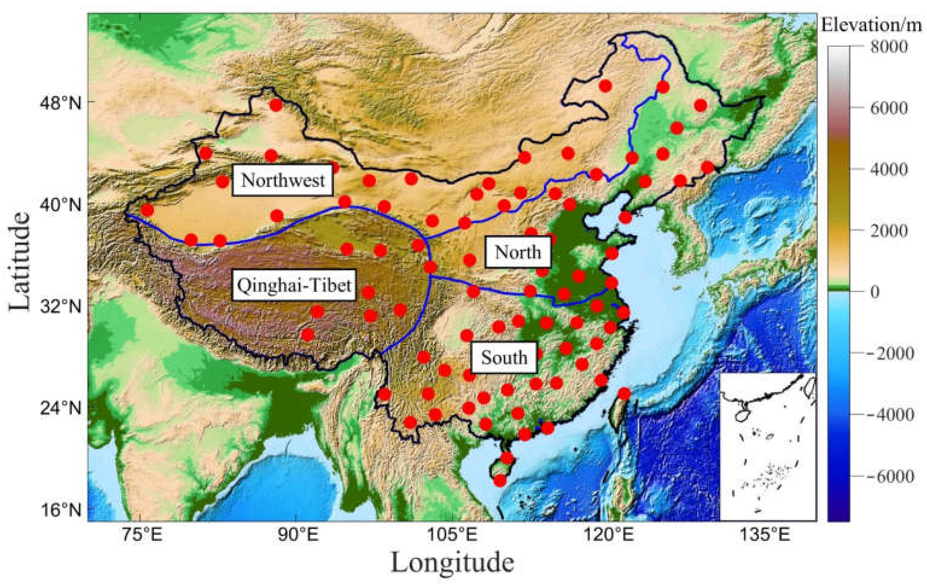
2.1. Data Description

RS data are derived from the RS dataset of the National Climatic Data Center, which is available from the Integrated Global Radiosonde Archive Version 2 (IGRA2) dataset. IGRA2 implemented several enhancements to accommodate characteristics that are not present in IGRA1 and to improve the quality of the final wind and humidity data. IGRA2 also includes more RS stations and longer recordings compared with IGRA1 [34]. This dataset covers almost 2700 global stations for both RS and pilot balloon observations dating from 1960 to present and can be downloaded for free online (ftp://ftp.ncdc.noaa.gov/pub/data/igra/, accessed on 1 July 2021) [35]. RS data can provide the vertical profiles of meteorological parameters, including temperature, geopotential, and water vapor pressure, usually two or four times a day [36]. In this paper, RS data with the temporal resolution of two times (UTC 00:00 and 12:00) daily are selected from 87 RS stations in China over the period between 2011 to 2020. Given that T_m is highly related to geographical location, this study divides China into four geographical divisions. Figure 1 presents the geographical distribution of the 87 selected RS stations and the four geographical divisions of China.

2.2. Data Pre-Processing

Given the influence of external conditions, outliers in time series are inevitable when collecting data using meteorological sensors. As these outliers can adversely affect the further analysis, they should be removed at the data preprocessing period [37,38]. Interquartile range (IQR) is a commonly used method for outlier detection whose principle is to arrange a group of observation data from smallest to largest and then divide them into quartiles. The data in the 25th and 75th percentiles represent the lower and upper quartiles, respectively and the difference between them represents the IQR [39,40], which can be expressed as

$${\mathrm{IQR}=\mathrm{Q}}_2{-\mathrm{Q}}_1$$

(1)

where ${\mathrm{Q}}_1$ is the lower quartile, ${\mathrm{Q}}_2$ is the upper quartile; ${(\mathrm{Q}}_1{,\mathrm{Q}}_2)$ covers the middlemost 50% of the data distribution. When the data fall in ${(\mathrm{Q}}_1-1.5*\mathrm{IQR},{\mathrm{Q}}_2+1.5*\mathrm{IQR})$, the data dispersion is low and can be regarded as normal values; otherwise, the data are rejected as outliers.

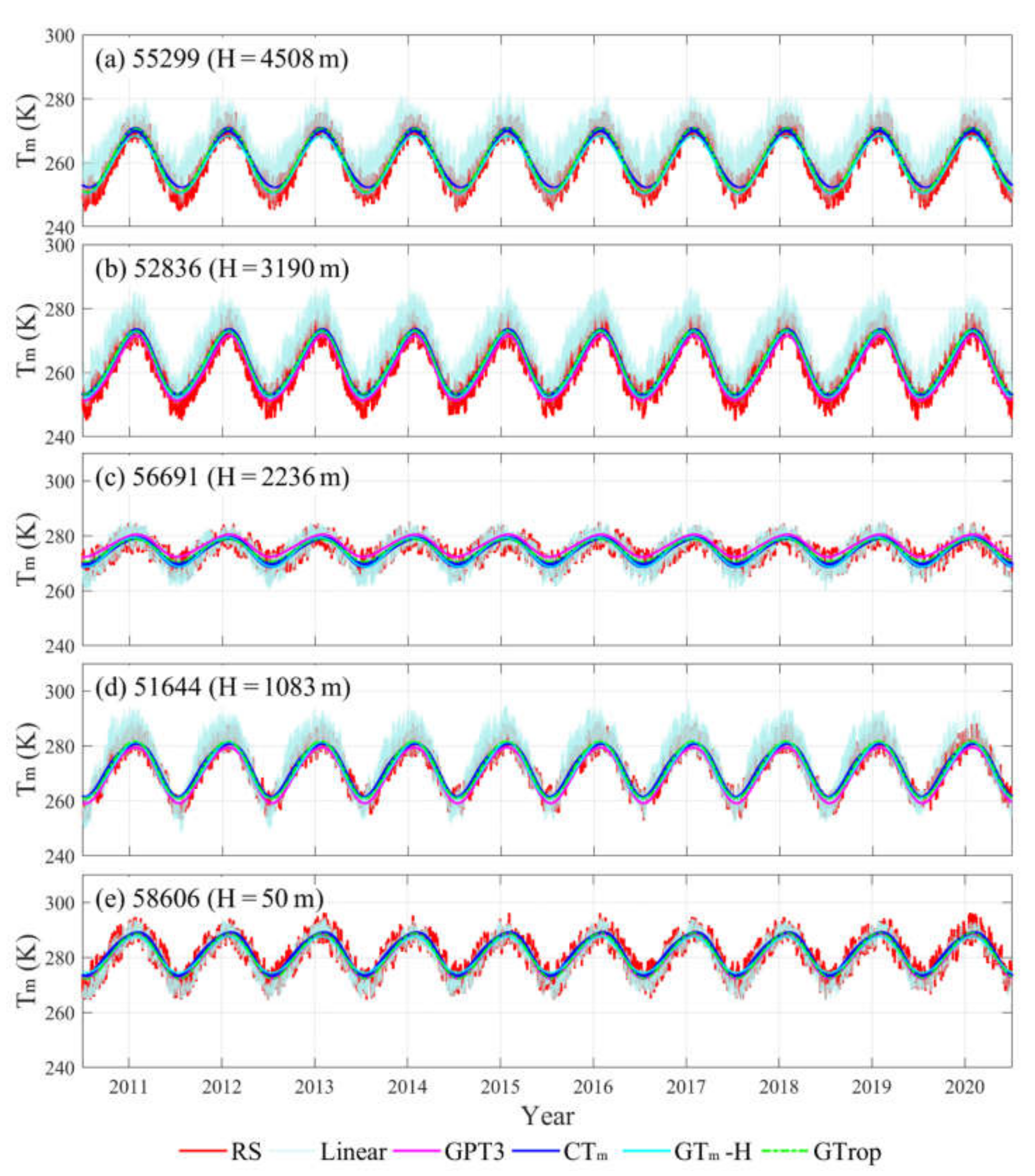
2.3. T_m Derived from RS Data

RS technology can obtain station-based meteorological parameters, such as temperature, pressure, potential height, and the relative humidity of different atmospheric layers. Given that these meteorological data are collected by meteorological sensors onboard an RS balloon, the T_m value calculated using these observed data has relatively high accuracy; Although RS has high accuracy in temperature profiles and uncertainty in humidity profiles, there is currently no better data source than RS for obtaining T_m, so RS can be considered as a reference for obtaining relatively better accuracy T_m [41]. RS provides meteorological data profiles in the form of layers and T_m is calculated as follows, according to the profile data of various meteorological parameters [42]:

$${\mathrm{T}}_{\mathrm{m}}=\frac{{\displaystyle \sum _{i=1}^n\frac{({\mathrm{z}}_2-{\mathrm{z}}_1){\mathrm{e}}_i}{{\mathrm{T}}_i}}}{{\displaystyle \sum _{i=1}^n\frac{({\mathrm{z}}_2-{\mathrm{z}}_1){\mathrm{e}}_i}{{\mathrm{T}}_i^2}}}$$

(2)

where ${\mathrm{z}}_1$ and ${\mathrm{z}}_2$ are the altitude values of the upper and lower observation layers, $\mathrm{e}$ and $\mathrm{T}$ are the water vapor pressure and temperature over the observation layers, respectively. Although the T_m calculated by RS has relatively good accuracy and can be used as a reference to evaluate the accuracy of the T_m model, there is uncertainty in the calculation of T_m due to the uncertainty in the humidity measurement and this approach has low spatial and temporal resolutions [43,44].

2.4. T_m Derived from Empirical Models

Five typical T_m models are selected in this paper, namely, the Linear, GPT3, CT_m, GT_m-H and GTrop models, to evaluate their accuracy in China.

Table 1. Input parameters and application areas of the five selected T_m models.

Models	Input Parameters	Applicable Area	Data	Period
Linear	Ts	China	RS	2011–2020
GPT3	lat., lon., altitude, time	Global	ECMWF, VLBI	1999–2014
CTm	lat., lon., altitude, time	China	GGOS	2007–2014
GTm-H	lat., lon., altitude, time	Global	ECMWF	2013–2015
GTrop	lat., lon., altitude, time	Global	ECMWF	1979–2017

presents detailed information about these models, including their input parameters, application area, data used for modeling and selected data period.

• Linear model

The Linear T_m model is established based on the linear regression equation of T_m and T_s. This model obtains T_m by simply inputting T_s at RS stations. In this paper, the linear relationship between T_m and T_s is established as follows using the RS data collected from 87 stations over the period of 2011 to 2020 in China:

$${\mathrm{T}}_{\mathrm{m}}=77.18+0.69{\mathrm{T}}_{\mathrm{s}}$$

(3)

where ${\mathrm{T}}_{\mathrm{s}}$ is the surface temperature.

2.

GPT3 model

GPT3 is a commonly used global pressure and temperature empirical model that provides various parameters, such as pressure, water vapor pressure, T_m, temperature lapse rate, mapping function and gradient. Given its simple calculation and relatively high accuracy on global scale, GPT3 has been widely used in the geodetic and meteorological fields [45,46]. This model calculates T_m as

$${\mathrm{T}}_{\mathrm{m}}{=\mathrm{A}}_0{+\mathrm{A}}_1\cos (\frac{\mathrm{DOY}}{365.25}{2\mathsf{\pi })+\mathrm{B}}_1\sin (\frac{\mathrm{DOY}}{365.25}{2\mathsf{\pi })+\mathrm{A}}_2\cos (\frac{\mathrm{DOY}}{365.25}{4\mathsf{\pi })+\mathrm{B}}_2\sin (\frac{\mathrm{DOY}}{365.25}4\mathsf{\pi })$$

(4)

where $\mathrm{DOY}$ is day of year, ${\mathrm{A}}_0$ is the mean value of ${\mathrm{T}}_{\mathrm{m}}$, ${\mathrm{A}}_1$ and ${\mathrm{B}}_1$ are the coefficients of annual amplitude and ${\mathrm{A}}_2$ and ${\mathrm{B}}_2$ are the coefficients of semi-annual amplitude. In the T_m calculation of the GPT3 model, the coefficients and their amplitudes could be saved as a grid, from which the user then could spatially interpolate the desired position.

3.

CT_m model

The CT_m model is a grid empirical model that considers the annual and semi-annual periodic signals of T_m and the relationship between T_m and altitude. This model initially calculates the T_m value at the altitude of the grid point and then normalizes the T_m of the four grid points around an RS station to the altitude of this station. In this model, T_m can be calculated by inputting the longitude, latitude, altitude, and time of a specific RS station. The T_m model expression at grid point altitude is the same as that in Equation (4) and the T_m at the four-grid point altitude around the station are unified to station altitude, which can be expressed as

$${\mathrm{T}}_{\mathrm{m}}^{\mathrm{U}}={\mathrm{T}}_{\mathrm{m}}^{\mathrm{G}}-\mathrm{g}\times ({\mathrm{H}}_{\mathrm{U}}-{\mathrm{H}}_{\mathrm{G}})$$

(5)

where ${\mathrm{T}}_{\mathrm{m}}^{\mathrm{U}}$ denotes the ${\mathrm{T}}_{\mathrm{m}}$ at the station altitude, ${\mathrm{T}}_{\mathrm{m}}^{\mathrm{G}}$ denotes the ${\mathrm{T}}_{\mathrm{m}}$ at the grid point altitude, ${\mathrm{H}}_{\mathrm{U}}$ and ${\mathrm{H}}_{\mathrm{G}}$ denote the altitude at the station and grid point, respectively and $\mathrm{g}$ is the vertical lapse rate of T_m. After that, bilinear interpolation is carried out for the ${\mathrm{T}}_{\mathrm{m}}^{\mathrm{U}}$ of the four grid points with a unified altitude and the ${\mathrm{T}}_{\mathrm{m}}$ at the RS station as calculated by the CT_m model is finally obtained.

4.

GT_m-H model

The GT_m-H model considers the nonlinear vertical reduction of T_m in high latitudes and describes the nonlinear variation of temperature on the T_m profile, which comprises two components, namely, the T_m at the mean sea level and the corrected value of T_m in the altitude direction. This model can be expressed as

$${\mathrm{T}}_{\mathrm{m}}{=\mathrm{T}}_{\mathrm{m}}^{\mathrm{MSL}}{+\mathrm{T}}_{\mathrm{m}}^{\mathrm{h}}$$

(6)

$${\mathrm{T}}_{\mathrm{m}}^{\mathrm{h}}{=\mathsf{\alpha }}_1{\mathrm{h}+\mathsf{\alpha }}_2\cos (\frac{2\mathsf{\pi }\mathrm{h}}{20}{)+\mathsf{\alpha }}_3\sin (\frac{2\mathsf{\pi }\mathrm{h}}{20})$$

(7)

where ${\mathrm{T}}_{\mathrm{m}}^{\mathrm{MSL}}$ is the ${\mathrm{T}}_{\mathrm{m}}$ at the mean sea level (K) that is calculated the same way as Equation (4), ${\mathrm{T}}_{\mathrm{m}}^{\mathrm{h}}$ is the ${\mathrm{T}}_{\mathrm{m}}$ altitude correction value (K), $\mathrm{h}$ is the altitude (km), $\mathsf{\alpha }$ is the fitting parameter, ${\mathsf{\alpha }}_1$ represents the linear part of ${\mathrm{T}}_{\mathrm{m}}^{\mathrm{h}}$, ${\mathsf{\alpha }}_2$ and ${\mathsf{\alpha }}_3$ represent the nonlinear part of ${\mathrm{T}}_{\mathrm{m}}^{\mathrm{h}}$.

5.

GTrop model

The GTrop model considers the seasonal variations of T_m and uses the ERA-Interim reanalysis data over the period of 1979 to 2017 for the model construction, which provides the T_m for a global 1° × 1° grid network [47]. This model calculates the T_m for each grid point as

$$\begin{array}{l}{\mathrm{T}}_{\mathrm{m}}{=[\mathrm{A}}_1{+\mathrm{A}}_2{(\mathrm{Y}-1980)+\mathrm{A}}_3\cos (\frac{\mathrm{DOY}}{365.25}{2\mathsf{\pi })+\mathrm{A}}_4\sin (\frac{\mathrm{DOY}}{365.25}{2\mathsf{\pi })+\mathrm{A}}_5\cos (\frac{\mathrm{DOY}}{365.25}{4\mathsf{\pi })+\mathrm{A}}_6\sin (\frac{\mathrm{DOY}}{365.25}4\mathsf{\pi }\left)\right]-\\ {[\mathrm{A}}_7{+\mathrm{A}}_8{(\mathrm{Y}-1980)+\mathrm{A}}_9\cos (\frac{\mathrm{DOY}}{365.25}{2\mathsf{\pi })+\mathrm{A}}_{10}\sin (\frac{\mathrm{DOY}}{365.25}{2\mathsf{\pi })+\mathrm{A}}_{11}\cos (\frac{\mathrm{DOY}}{365.25}{4\mathsf{\pi })+\mathrm{A}}_{12}\sin (\frac{\mathrm{DOY}}{365.25}{4\mathsf{\pi }\left)\right](\mathrm{h}-\mathrm{h}}_0)\end{array}$$

(8)

where $\mathrm{Y}$ denotes year, ${\mathrm{h}}_0$ is the altitude at the grid point (km), $\mathrm{h}$ is the altitude at the station (km) and $\mathrm{A}(\mathrm{i}=1~12)$ is the model coefficients of T_m. The T_m of a specific station is obtained via bilinear interpolation from the four nearby grid points of the station altitude.

2.5. Statistical Metrics for T_m Model Evaluation

The T_m values derived from 87 RS stations are used as reference in evaluating the accuracy of the five typical models in China. The performance of these models is evaluated across different altitudes, latitudes, and geographical areas and over the entire area of China. Three evaluation indices are determined, namely, the root mean square (RMS), standard deviation (STD) and Bias. The standard deviation is used to measure the dispersion of a group of numbers, the RMS is used to measure the deviation between the observed value and the true value, and the Bias, is the average of the difference between the measured value and the true value. If the statistical distribution of the error is normal, then the probability of random error falling within ±σ is 68%. The corresponding indices are computed as

$$\mathrm{RMS}=\sqrt{\frac{1}{\mathrm{n}}{\displaystyle \sum _{\mathrm{i}=1}^{\mathrm{n}}{\mathrm{v}}_{\mathrm{i}}^2}}$$

(9)

$$\mathrm{Bias}=\frac{1}{\mathrm{n}}{\displaystyle \sum _{\mathrm{i}=1}^{\mathrm{n}}{\mathrm{v}}_{\mathrm{i}}}$$

(10)

$$\mathrm{STD}=\sqrt{\frac{1}{\mathrm{n}}{\displaystyle \sum _{\mathrm{i}=1}^{\mathrm{n}}{({\mathrm{x}}_{\mathrm{i}}-\mathrm{u})}^2}}$$

(11)

where ${\mathrm{v}}_{\mathrm{i}}$ is the difference between the T_m derived from the empirical T_m models and RS data, and $\mathrm{n}$ is the total number of observed values. $\mathrm{RMS}$ is used to evaluate the overall accuracy of the empirical T_m models, whereas $\mathrm{Bias}$ is used to evaluate their average deviation. ${\mathrm{x}}_{\mathrm{i}}$ is the T_m derived from the empirical T_m models and $\mathrm{u}$ is its average value.

3. Accuracy Analysis of T_m Models

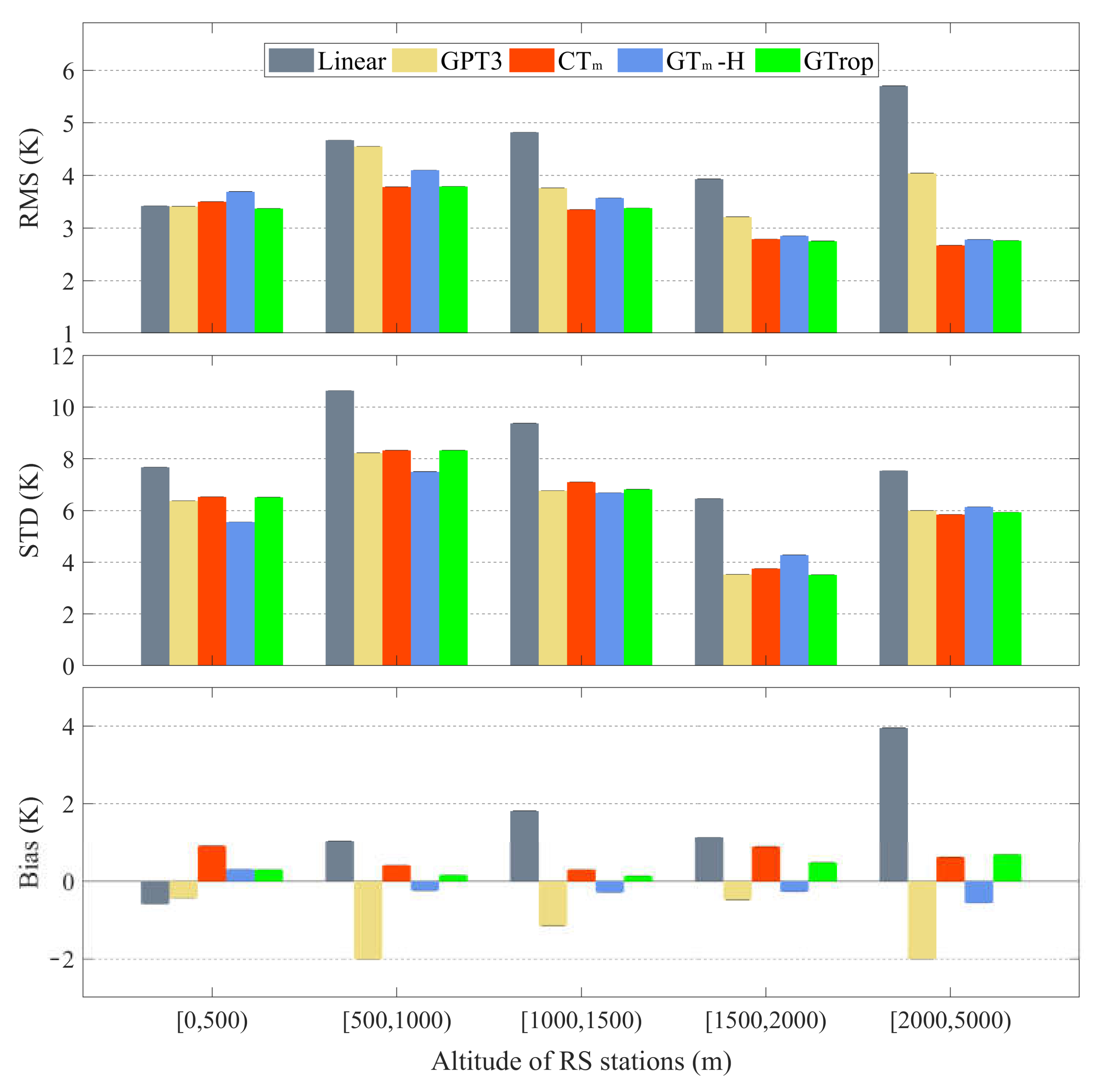
3.1. Accuracy Analysis at Different Altitudes

To verify the accuracy of the five typical T_m models at different altitudes, five RS stations with station names of 55299, 52836, 56691, 51644 and 58606 distributed in different altitudes are selected and the time series of T_m derived from the five models and the selected RS stations over the period of 2011 to 2020 are compared (Figure 2). As can be seen from Figure 2, the T_m value gradually decreases along with an increasing altitude. The T_m derived from the five models are generally consistent with that derived by the RS stations, but the corresponding values from the Linear model tend to be large at high altitudes. To further analyze the performance of these models in different altitudes, 87 RS stations in China are divided into five groups according to different altitudes, namely, [0, 500), [500, 1000), [1000, 1500), [1500, 2000) and [2000, 5000). Figure 3 presents the average RMS, STD, and Bias values for each group of RS stations over the period of 2011 to 2020. Comparison results show that the errors of the Linear model at different altitudes are all large and gradually increase along with altitude. A significant positive deviation and a large RMS are also observed in the altitude range, hence suggesting that the Linear model is not suitable for calculating T_m in high-altitude regions. The T_m derived from GPT3 model also shows a large RMS at altitudes exceeding 500 m. Meanwhile, the Bias results show that the T_m derived from the GPT3 model demonstrate obvious negative deviations at different altitudes. Among the five T_m models, CT_m, GT_m-H and GTrop models have the most stable accuracy, and their accuracy is significantly higher at altitudes exceeding 2000 m because they consider the effect of altitude on T_m. In addition, the T_m derived from Linear model shows the largest error among all models at different altitudes, followed by the GPT3 model. Meanwhile, the CT_m, GT_m-H and GTrop models obtain relatively high accuracy, and their RMS tends to decrease along with increasing altitude and their Bias values are all less than 1 K at different altitudes. In general, GTrop model has the smallest RMS at different altitudes, which indicates its high accuracy and stability. The Linear and GTrop models do not greatly differ in their RMS value, which is around 3.5 K. However, with an increasing altitude, the RMS of these models shows an opposite trend. In the [2000, 5000) group, the RMS derived from Linear model reaches 5.7 K, whereas that of the GTrop model reaches only 2.7 K. The same difference between the Linear and GTrop model can also be observed in their Bias values. In the [2000, 5000) group, the Bias value of the Linear model reaches 4.0 K, whereas that of the GTrop model falls within the range of (0, 1) K at different altitudes. Therefore, at different altitudes, the GTrop model shows a larger advantage than the traditional model, while in the [2000, 5000) group, the CT_m model has relatively better accuracy.

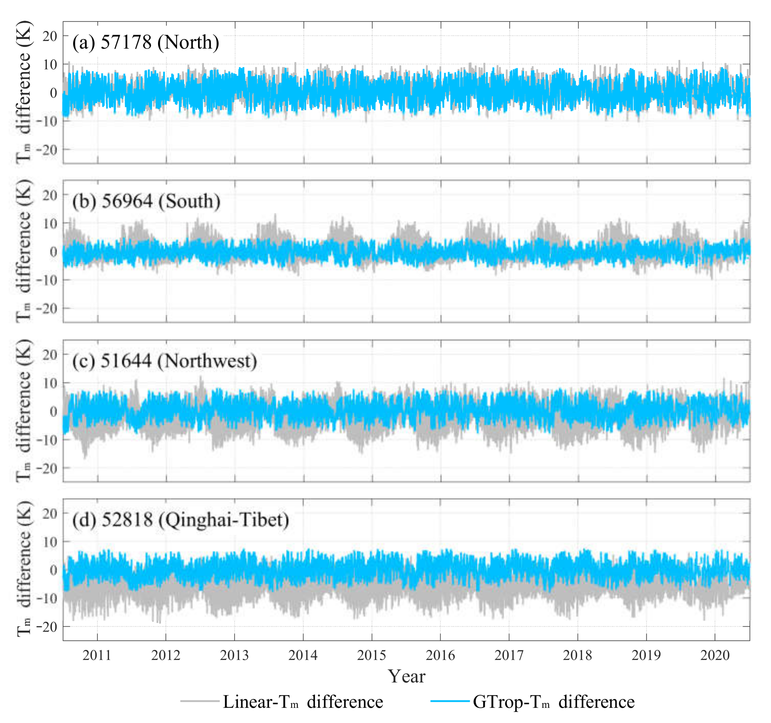
3.2. Accuracy Analysis at Different Latitudes

To further verify the accuracy of the five T_m models at different latitudes, 87 RS stations in China are divided into six groups, namely, [15°, 25°), [25°, 30°), [30°, 35°), [35°, 40°), [40°, 45°) and [45°, 55°), according to their latitude. Figure 4 presents a time series comparison of the five typical T_m models at six RS stations with station names of 50774, 53068, 52866, 56146, 58633 and 59265 in different latitude groups. It can be observed that the T_m gradually decreases along with increasing latitude. In the low latitude region, the T_m derived by these models shows good consistency with that derived from the RS stations, but some differences are observed in the mid-latitude and high latitude regions, especially between the Linear and GPT3 model. Figure 5 presents the average RMS, STD and Bias statistics of these models at different latitudes over the period of 2011 to 2020. These five models obtain different accuracies across each latitude. In terms of RMS, the RMS of the five T_m models gradually increase along with latitude, the RMS of the Linear model is relatively large at different latitudes, the RMS of the CT_m and GTrop models are small and do not increase much and the GT_m-H model obtains a relatively large RMS at high latitudes [45°, 55°). Meanwhile, the Bias comparison results show that the Linear model has a negative deviation in T_m at low latitudes and a positive deviation at mid- and high latitudes, the GPT3 model has negative deviations at different latitudes and the GT_m-H and GTrop models have deviations of less than 1 K at different latitudes, especially at the mid- and high latitude regions where these models report smaller deviations compared with the other models. In addition, the errors of the five T_m models gradually increase along with latitude. In general, both GTrop and CT_m models show relatively good performance at different latitudes. The RMS of CT_m is slightly smaller than that of GTrop model at middle latitudes [35°, 40°), but GTrop model is better than CT_m model from the perspective of Bias index.

3.3. Accuracy Analysis at Different Geographical Regions in China

Given that T_m is affected by different locations and natural environments [48], China is divided into four geographical regions, namely, North (N), South (S), Northwest (NW) and Qinghai-Tibet (QT), to analyze the performance of the five typical T_m models. These regions have average altitudes of 0.3, 0.5, 1.1 and 3.3 km, respectively. A total of 20, 34, 24 and nine RS stations are distributed in regions of N, S, NW and QT, respectively. To evaluate the accuracy of the traditional and empirical models, Figure 6 shows the time series of T_m differences derived from the Linear and GTrop models at four RS stations with station names of 57178, 56964, 51644 and 52818 distributed in regions of N, S, NW, and QT over the period of 2011 to 2020. The T_m values derived by these empirical models exhibit some differences in four geographical regions of China. For instance, the T_m difference derived from the GTrop model is smaller than that of the Linear model, especially in the NW and QT regions but not in the N region. Therefore, the GTrop model should be used instead of the traditional Linear model in the QT region to obtain T_m with relatively better accuracy. Figure 7 shows the RMS and absolute Bias (ABias) of the five T_m models in four geographical regions. Here, the RMS and Abias presented in Figure 7 was calculated using all radiosonde stations located in each region. The accuracy of the T_m models shows different characteristics in each region. Specifically, the RMS values of these models in regions of N and NW are larger than those in region of S. Across all four geographical regions, the Linear model obtains the largest RMS value among all those models. This model also obtains the largest ABias value in regions of S and QT. Generally, the CT_m and GTrop models outperform the other empirical T_m models in the four geographical regions of China.

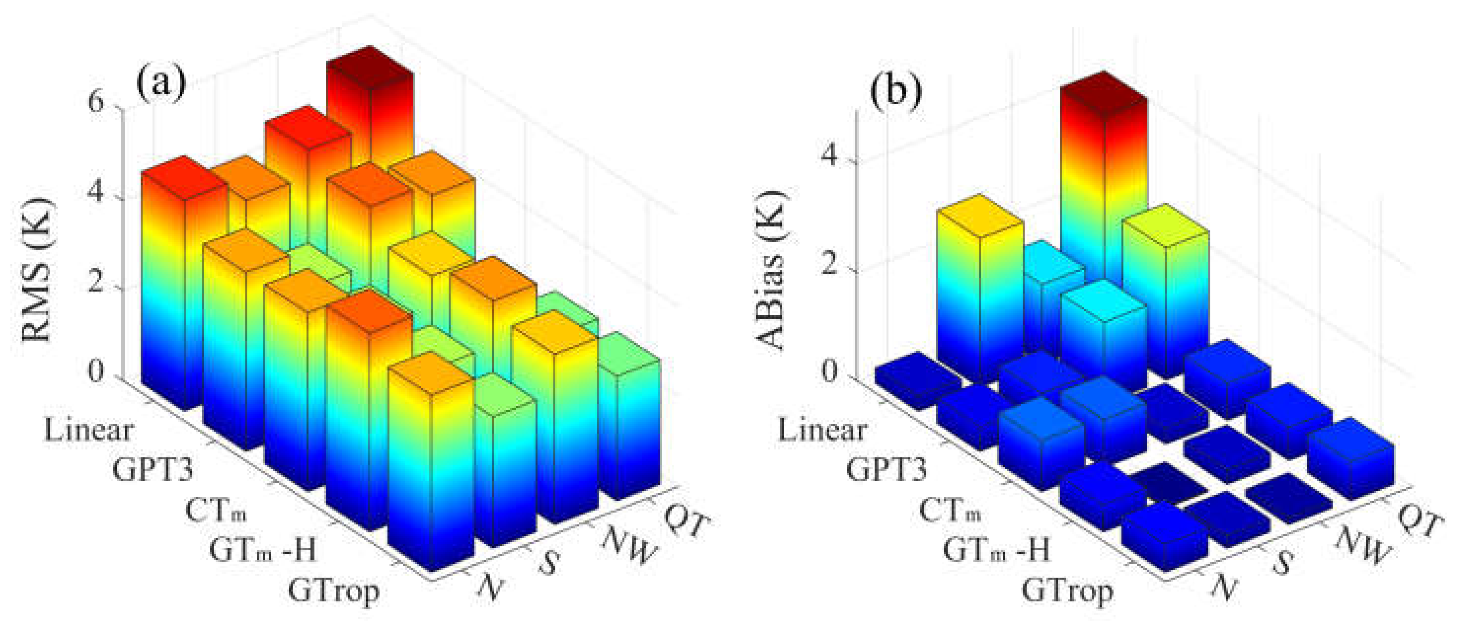
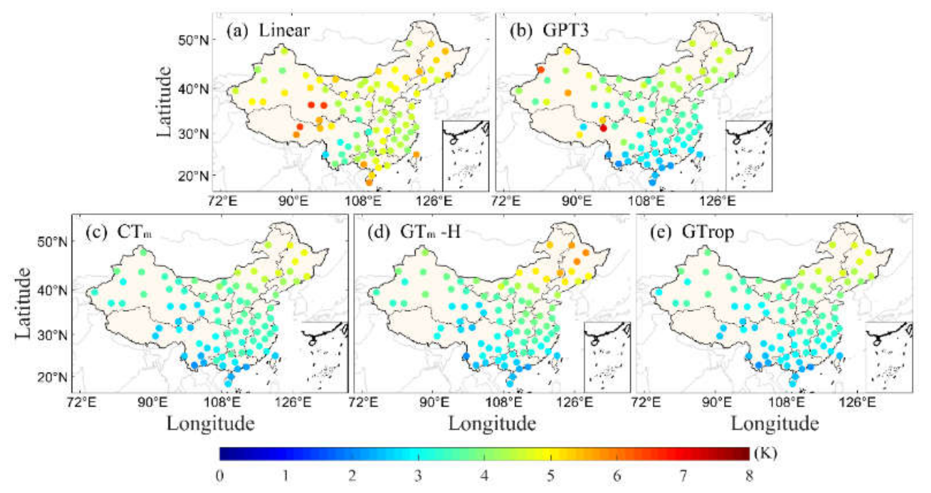
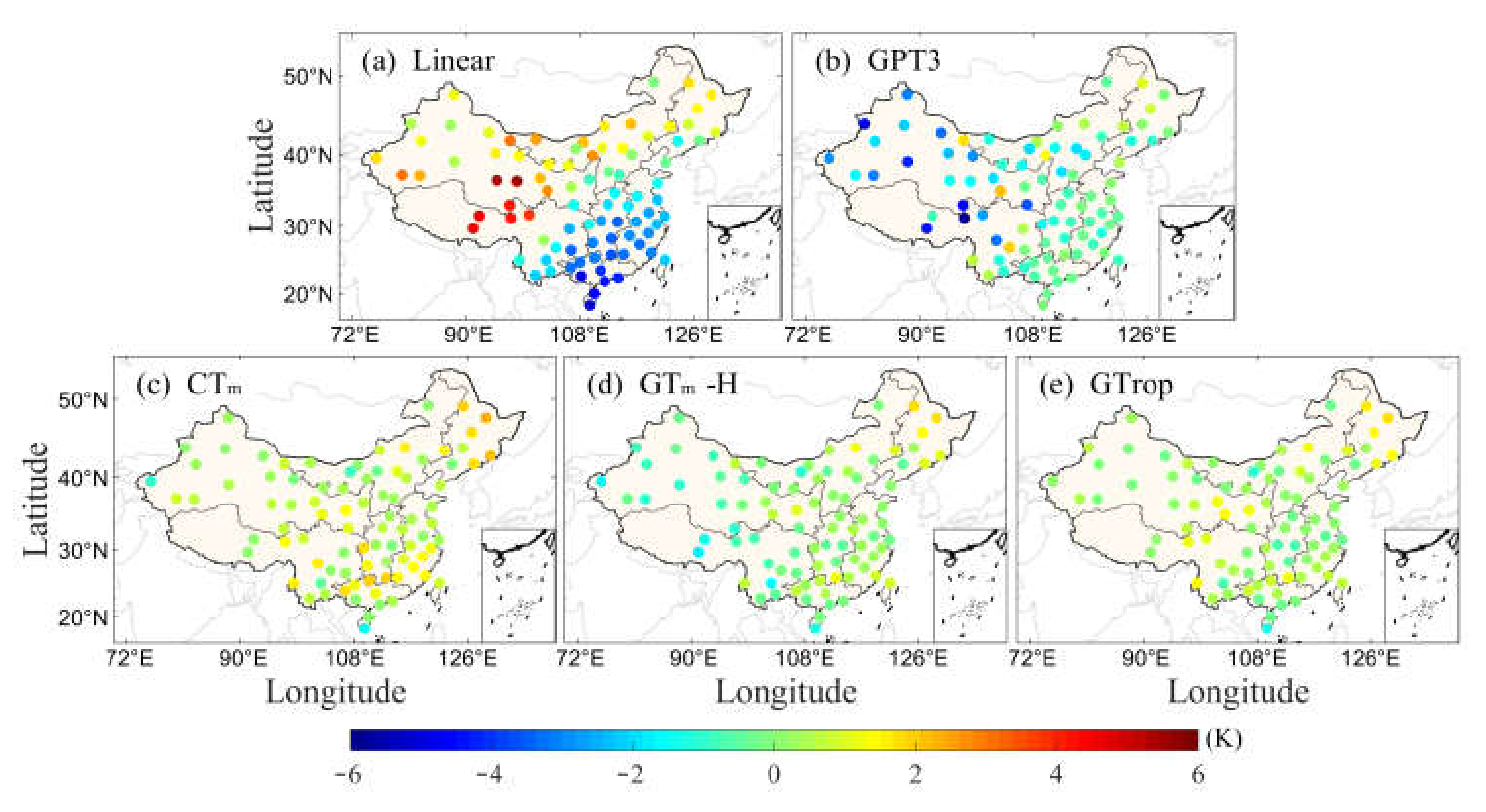
3.4. Overall Evaluation of T_m Models in China

To validate the overall accuracy of the five typical T_m models in China, the corresponding T_m values at 87 RS stations in China over the period of 2011 to 2020 are compared with those derived by the empirical models. Figure 8 and Figure 9 present RMS and Bias distributions of T_m difference between the RS and five typical T_m models, respectively. It can be observed that the CT_m and GTrop models show the best accuracy at high-altitude regions, whereas the Linear model present the lowest accuracy. The Bias of the Linear model is obviously large in NW region and smaller in S region of China, whereas that of GPT3 model is significantly smaller in NW. In addition, the ABias of the GT_m-H model is larger than that of the CT_m and GTrop models in QT region of China. In general, these empirical T_m models have better accuracy in low-latitude regions than in high-latitude regions.

Figure 10 and Figure 11 present the percentages of RMS and Bias in different intervals as calculated by the five T_m models at 87 RS stations in China. It can be observed that the Linear model has a relatively large number of RS stations with large RMS and Bias values. Meanwhile, the GPT3 and G_Tm-H models have relatively few stations with RMS values exceeding 5 K, whereas the RMS value of CT_m and GTrop models is below 5 K. In addition, there are more stations with RMS value of T_m derived from GTrop model less than 3 K. The Bias values in the CT_m, GT_m-H and GTrop models are concentrated in (−1, 1) K, whereas that in the Linear and GPT3 models are below (−1, 1) K. Generally, the CT_m, GT_m-H and GTrop models have relatively better accuracy than that of the other models.

Table 2. Average RMS and Bias of the five T_m models at 87 RS stations over the period of 2011 to 2020.

Model	RMS (K)			Bias (K)
	Max.	Min.	Aver.	Max.	Min.	Aver.
Linear	7.1	2.1	4.2	5.9	−2.8	0.7
GPT3	7.1	2.1	3.7	2.1	−6.7	−1.0
CTm	4.9	2.1	3.4	2.3	−1.4	0.7
GTm-H	5.8	2.0	3.6	1.9	−1.8	−0.1
GTrop	4.7	2.1	3.3	1.7	−1.4	0.3

shows that the average RMS of the five models are 4.2, 3.7, 3.4, 3.6 and 3.3 K for the 87 stations, whereas their average Bias are 0.7, −1.0, 0.7, −0.1 and 0.3 K, respectively. Generally, the GTrop model has the best accuracy among the five models followed by the CT_m model, whereas the Linear model demonstrates the worst accuracy.

4. Conclusions

To determine the optimal T_m model to be used in China, the performances of five typical T_m models, namely, Linear, GPT3, CT_m, GT_m-H and GTrop models, are compared and validated in this paper. Corresponding meteorological data of 87 RS stations over the period of 2011 to 2020 are selected to calculated T_m and as the reference. Although there is uncertainty, the RS measurements is based on LoCo technique and therefore can be considered the best for this evaluation. The performance and applicability of these T_m models are analyzed across different altitudes, latitudes, and geographical regions and for the entire China. Experimental results reveal that T_m shows obvious geographical characteristics in China and the accuracy of the selected T_m models generally decrease along with increasing altitude and latitude. The results obtained at different altitudes show that the Linear and GPT3 models are not suitable for calculating T_m in high-altitude regions, whereas the CT_m, GT_m-H and GTrop models have relatively good accuracy due to their consideration of the effects of altitude. In addition, the GTrop model has relatively more advantages over the other models in terms of accuracy and stability. Meanwhile, the results obtained at different latitudes reveal that these empirical T_m models show higher accuracies in low-latitude areas, but such accuracy decreases in the mid and high latitudes. The Linear and GPT3 models have large errors, whereas the GT_m-H and CT_m models obtain high accuracy in high latitudes. Results obtained at different geographical regions also verified the relatively higher accuracy and stability of the GTrop model compared with the other T_m models. Therefore, the GTrop model is recommended for calculating T_m in China.

References

1. Zhao, Q.; Liu, Y.; Yao, W.; Yao, Y. Hourly rainfall forecast model using supervised learning algorithm. IEEE Trans. Geosci. Remote Sens. 2021, 60, 4100509. [Google Scholar] [CrossRef]
2. Zhao, Q.; Liu, Y.; Ma, X.; Yao, W.; Yao, Y.; Li, L. An improved rainfall forecasting model based on GNSS observations. IEEE Trans. Geosci. Remote Sens. 2020, 58, 4891–4900. [Google Scholar] [CrossRef]
3. Huang, L.; Liu, L.; Chen, H.; Jiang, W. An improved atmospheric weighted mean temperature model and its impact on GNSS precipitable water vapor estimates for China. GPS Solut. 2019, 23, 51. [Google Scholar] [CrossRef]
4. Yao, Y.; Sun, Z.; Xu, C. Applicability of Bevis Formula at Different Height Levels and Global Weighted Mean Temperature Model Based on Near-earth Atmospheric Temperature. J. Geod. Geoinf. Sci. 2020, 3, 1–11. [Google Scholar]
5. Lee, S.-W.; Choi, B.I.; Woo, S.-B.; Kim, J.C.; Kim, Y.-G. Calibration of a radiosonde humidity sensor at low temperature and low pressure. Metrologia 2019, 56, 055008. [Google Scholar] [CrossRef]
6. Zhao, Q.; Ma, X.; Yao, W.; Liu, Y.; Yao, Y. A drought monitoring method based on precipitable water vapor and precipitation. J. Clim. 2020, 33, 10727–10741. [Google Scholar] [CrossRef]
7. Zhao, Q.; Du, Z.; Li, Z.; Yao, W.; Yao, Y. Two-Step Precipitable Water Vapor Fusion Method. IEEE Trans. Geosci. Remote Sens. 2021, 60, 5801510. [Google Scholar] [CrossRef]
8. Yao, Y.; Xu, C.; Zhang, B.; Cao, N. GTm-III: A new global empirical model for mapping zenith wet delays onto precipitable water vapour. Geophys. J. Int. 2014, 197, 202–212. [Google Scholar] [CrossRef] [Green Version]
9. Huang, L.; Jiang, W.; Liu, L.; Chen, H.; Ye, S. A new global grid model for the determination of atmospheric weighted mean temperature in GPS precipitable water vapor. J. Geod. 2019, 93, 159–176. [Google Scholar] [CrossRef]
10. Ding, M.; Hu, W. A further contribution to the seasonal variation of weighted mean temperature. Adv. Space Res. 2017, 60, 2414–2422. [Google Scholar] [CrossRef]
11. Bevis, M.; Businger, S.; Herring, T.A.; Rocken, C.; Anthes, R.A.; Ware, R.H. GPS meteorology: Remote sensing of atmospheric water vapor using the Global Positioning System. J. Geophys. Res. Atmos. 1992, 97, 15787–15801. [Google Scholar] [CrossRef]
12. Ding, M. A neural network model for predicting weighted mean temperature. J. Geod. 2018, 92, 1187–1198. [Google Scholar] [CrossRef]
13. Yang, F.; Guo, J.; Meng, X.; Shi, J.; Zhang, D.; Zhao, Y. An improved weighted mean temperature (Tm) model based on GPT2w with Tm lapse rate. GPS Solut. 2020, 24, 46. [Google Scholar] [CrossRef]
14. Gao, W.; Gao, J.; Yang, L.; Wang, M.; Yao, W. A novel modeling strategy of weighted mean temperature in China using RNN and LSTM. Remote Sens. 2021, 13, 3004. [Google Scholar] [CrossRef]
15. Böhm, J.; Heinkelmann, R.; Schuh, H. Short note: A global model of pressure and temperature for geodetic applications. J. Geod. 2007, 81, 679–683. [Google Scholar] [CrossRef]
16. Lagler, K.; Schindelegger, M.; Böhm, J.; Krásná, H.; Nilsson, T. GPT2: Empirical slant delay model for radio space geodetic techniques. Geophys. Res. Lett. 2013, 40, 1069–1073. [Google Scholar] [CrossRef] [Green Version]
17. Böhm, J.; Möller, G.; Schindelegger, M.; Pain, G.; Weber, R. Development of an improved empirical model for slant delays in the troposphere (GPT2w). GPS Solut. 2015, 19, 433–441. [Google Scholar] [CrossRef] [Green Version]
18. Yao, Y.B.; Zhang, B.; Yue, S.Q.; Xu, C.Q.; Peng, E.F. Global empirical model for mapping zenith wet delays onto precipitable water. J. Geod. 2013, 87, 439–448. [Google Scholar] [CrossRef]
19. Yao, Y.; Zhang, B.; Xu, C.; Yan, F. Improved one/multi-parameter models that consider seasonal and geographic variations for estimating weighted mean temperature in ground-based GPS meteorology. J. Geod. 2014, 88, 273–282. [Google Scholar] [CrossRef]
20. Sun, Z.; Zhang, B.; Yao, Y. A global model for estimating tropospheric delay and weighted mean temperature developed with atmospheric reanalysis data from 1979 to 2017. Remote Sens. 2019, 11, 1893. [Google Scholar] [CrossRef] [Green Version]
21. Huang, L.; Peng, H.; Liu, L.; Li, C.; Kang, C.; Xie, S. An empirical atmospheric weighted mean temperature model considering the lapse rate function for China. Acta Geod. Cartogr. Sin. 2020, 49, 432–442. [Google Scholar]
22. Landskron, D.; Böhm, J. VMF3/GPT3: Refined discrete and empirical troposphere mapping functions. J. Geod. 2018, 92, 349–360. [Google Scholar] [CrossRef]
23. Nistor, S.; Suba, N.S.; Buda, A.S. The impact of tropospheric mapping function on PPP determination for one-month period. Acta Geodyn. Geomater. 2020, 17, 237–252. [Google Scholar] [CrossRef]
24. Mao, J.; Han, J.; Cui, T. Development and Assessment of Improved Global Pressure and Temperature Series Models. IEEE Access 2021, 9, 104429–104447. [Google Scholar] [CrossRef]
25. Li, T.; Wang, L.; Chen, R.; Fu, E.; Xu, W.; Jiang, P.; Liu, J.; Zhou, H.; Han, Y. Refining the empirical global pressure and temperature model with the ERA5 reanalysis and radiosonde data. J. Geod. 2021, 95, 31. [Google Scholar] [CrossRef]
26. Yao, Y.; Sun, Z.; Xu, C.; Xu, X. Global Weighted Mean Temperature Model Considering Nonlinear Vertical Reduction. Geomat. Inf. Sci. Wuhan Univ. 2019, 44, 106–111. [Google Scholar]
27. Zhu, M.; Hu, W.; Sun, W. Advanced grid model of weighted mean temperature based on feedforward neural network over China. Earth Space Sci. 2021, 8, e2020EA001458. [Google Scholar] [CrossRef]
28. Huang, L.; Zhu, G.; Liu, L.; Chen, H.; Jiang, W. A global grid model for the correction of the vertical zenith total delay based on a sliding window algorithm. GPS Solut. 2021, 25, 98. [Google Scholar] [CrossRef]
29. Mo, Z.X.; Huang, L.K.; Peng, H.; Liu, L.L.; Kang, C.L. Atmospheric Weighted Mean Temperature Model in Guilin. Int. Arch. Photogramm. Remote Sens. Spat. Inf. Sci. 2020, 42, 1155–1160. [Google Scholar] [CrossRef] [Green Version]
30. Huang, L.; Mo, Z.; Liu, L.; Xie, S. An empirical model for the vertical correction of precipitable water vapor considering the time-varying lapse rate for Mainland China. Acta Geod. Cartogr. Sin. 2021, 50, 1320–1330. [Google Scholar]
31. Gao, Z.; He, X.; Chang, L. Accuracy Analysis of GPT3 Model in China. Geomat. Inf. Sci. Wuhan Univ. 2021, 46, 538–545. [Google Scholar]
32. Zhu, H.; Chen, K.; Huang, G. A Weighted Mean Temperature Model with Nonlinear Elevation Correction Using China as an Example. Remote Sens. 2021, 13, 3887. [Google Scholar] [CrossRef]
33. Long, F.; Gao, C.; Yan, Y.; Wang, J. Enhanced neural network model for worldwide estimation of weighted mean temperature. Remote Sens. 2021, 13, 2405. [Google Scholar] [CrossRef]
34. Durre, I.; Yin, X.; Vose, R.S.; Applequist, S.; Arnfield, J. Enhancing the data coverage in the integrated global radiosonde archive. J. Atmos. Ocean. Technol. 2018, 35, 1753–1770. [Google Scholar] [CrossRef]
35. Makama, E.K.; Lim, H.S. Variability and Trend in Integrated Water Vapour from ERA-Interim and IGRA2 Observations over Peninsular Malaysia. Atmosphere 2020, 11, 1012. [Google Scholar] [CrossRef]
36. Zhao, Q.; Yang, P.; Yao, W.; Yao, W. Adaptive AOD Forecast Model Based on GNSS-Derived PWV and Meteorological Parameters. IEEE Trans. Geosci. Remote Sens. 2021, 60, 5800610. [Google Scholar] [CrossRef]
37. Martin, A.; Weissmann, M.; Reitebuch, O.; Rennie, R.; Geiß, A.; Cress, A. Validation of Aeolus winds using radiosonde observations and numerical weather prediction model equivalents. Atmos. Meas. Tech. 2021, 14, 2167–2183. [Google Scholar] [CrossRef]
38. Zhao, Q.; Su, J.; Li, Z.; Yang, P.; Yao, Y. Adaptive aerosol optical depth forecasting model using GNSS observation. IEEE Trans. Geosci. Remote Sens. 2021, 60, 4105009. [Google Scholar] [CrossRef]
39. Van Zoest, V.M.; Stein, A.; Hoek, G. Outlier detection in urban air quality sensor networks. Water Air Soil Pollut. 2018, 229, 111. [Google Scholar] [CrossRef] [Green Version]
40. Bărbulescu, A.; Dumitriu, C.S.; Ilie, I.; Barbeş, S.-B. Influence of Anomalies on the Models for Nitrogen Oxides and Ozone Series. Atmosphere 2022, 13, 558. [Google Scholar]
41. Li, L.; Li, Y.; He, Q.; Wang, X. Weighted Mean Temperature Modelling Using Regional Radiosonde Observations for the Yangtze River Delta Region in China. Remote Sens. 2022, 14, 1909. [Google Scholar] [CrossRef]
42. Czernecki, B.; Głogowski, A.; Nowosad, J. Climate: An R package to access free in-situ meteorological and hydrological datasets for environmental assessment. Sustainability 2020, 12, 394. [Google Scholar] [CrossRef] [Green Version]
43. Sun, Z.; Zhang, B.; Yao, Y. An ERA5-based model for estimating tropospheric delay and weighted mean temperature over China with improved spatiotemporal resolutions. Earth Space Sci. 2019, 6, 1926–1941. [Google Scholar] [CrossRef]
44. Choi, B.I.; Lee, S.W.; Woo, S.B.; Kim, J.C.; Kim, Y.-G.; Yang, S.G. Evaluation of radiosonde humidity sensors at low temperature using ultralow-temperature humidity chamber. Adv. Sci. Res. 2018, 15, 207–212. [Google Scholar] [CrossRef]
45. Ding, J.; Chen, J. Assessment of empirical troposphere model GPT3 based on NGL’s global troposphere products. Sensors 2020, 20, 3631. [Google Scholar] [CrossRef]
46. Li, J.; Zhang, B.; Yao, Y.; Liu, L.; Sun, Z.; Yan, X. A refined regional model for estimating pressure, temperature and water vapor pressure for geodetic applications in China. Remote Sens. 2020, 12, 1713. [Google Scholar] [CrossRef]
47. Ding, M. A second generation of the neural network model for predicting weighted mean temperature. GPS Solut. 2020, 24, 61. [Google Scholar] [CrossRef]
48. Yu, H.; Miao, S.; Xie, G.; Guo, X.; Chen, Z.; Favre, A. Contrasting floristic diversity of the Hengduan Mountains, the Himalayas and the Qinghai-Tibet Plateau sensu stricto in China. Front. Ecol. Evol. 2020, 8, 136. [Google Scholar] [CrossRef]
Figure 1. Geographical distribution of the 87 selected RS stations and the four geographical divisions of China.
Remotesensing 14 03435 g001
Figure 2. Time series comparison of the five Tm models and the RS-derived Tm at five stations distributed in different altitudes over the period of 2011 to 2020.
Remotesensing 14 03435 g002
Figure 3. Average RMS and Bias of the five Tm models at different altitude ranges over the period of 2011 to 2020.
Remotesensing 14 03435 g003
Figure 4. Time series comparison of the five Tm models and the RS-derived Tm at six stations distributed in different latitudes over the period of 2011 to 2020.
Remotesensing 14 03435 g004
Figure 5. Average RMS and Bias of the five Tm models at different latitudes over the period of 2011 to 2020.
Remotesensing 14 03435 g005
Figure 6. Comparison of Tm difference between the Linear/GTrop model and four RS stations distributed across the four geographical regions of China over the period of 2011 to 2020.
Remotesensing 14 03435 g006
Figure 7. Average RMS and absolute Bias (ABias) of the five Tm models in the four geographical regions of China over the period of 2011 to 2020. (a) refers average RMS of the five Tm models in the four geographical regions of China over the period of 2011 to 2020 and (b) refers absolute Bias (ABias) of the five Tm models in the four geographical regions of China over the period of 2011 to 2020.
Remotesensing 14 03435 g007
Figure 8. RMS distribution of the Tm difference between the five Tm models and the 87 RS stations in China over the period of 2011 to 2020.
Remotesensing 14 03435 g008
Figure 9. Bias distribution of the Tm difference between the five Tm models and the 87 RS stations in China over the period of 2011 to 2020.
Remotesensing 14 03435 g009
Figure 10. Percentage of RMS in different intervals calculated by the five Tm models at 87 RS stations over the period of 2011 to 2020.
Remotesensing 14 03435 g010
Figure 11. Percentage of Bias in different intervals calculated by the five Tm models at 87 RS stations over the period of 2011 to 2020.
Remotesensing 14 03435 g011