LGB-PHY: An Evaporation Duct Height Prediction Model Based on Physically Constrained LightGBM Algorithm

Abstract

The evaporation duct is a special atmospheric stratification that significantly influences the propagation path of electromagnetic waves at sea, and hence, it is crucial for the stability of the radio communication systems. Affected by physical parameters that are not universal, traditional evaporation duct theoretical models often have limited accuracy and poor generalization ability, e.g., the remote sensing method is limited by the inversion algorithm. The accuracy, generalization ability and scientific interpretability of the existing pure data-driven evaporation duct height prediction models still need to be improved. To address these issues, in this paper, we use the voyage observation data and propose the physically constrained LightGBM evaporation duct height prediction model (LGB-PHY). The proposed model integrates the Babin–Young–Carton (BYC) physical model into a custom loss function. Compared with the eXtreme Gradient Boosting (XGB) model, the LGB-PHY based on a 5-day voyage data set of the South China Sea provides significant improvement where the RMSE index is reduced by 68%, while the SCC index is improved by 6.5%. We further carried out a cross-comparison experiment of regional generalization and show that in the sea area with high latitude and strong adaptability of the BYC model, the LGB-PHY model has a stronger regional generalization performance than that of the XGB model.

1. Introduction

The atmospheric duct is a stratification in the atmospheric boundary layer which significantly affects the propagation of electromagnetic waves. This is because the refractive index in the atmospheric boundary layer is sharply decreased with the increase in altitude. Therefore, the electromagnetic waves may abnormally bend downward, resulting in the bending radius of the waves becoming smaller than that of the earth. For some frequencies and angle conditions, the energy of radio waves will be refracted repeatedly in the atmospheric stratification. Hence, the atmospheric stratification acts as a conductor that enables low attenuation over-the-horizon propagation of electromagnetic waves. Nonetheless, this limits the transmission of electromagnetic waves only within the atmospheric duct. Figure 1 shows the radar blind zone caused by the atmosphere duct. Efficient use of the atmospheric duct not only improves radio communications between the ships at sea but also shields the communication equipment in the air from radio interference.

The atmospheric duct includes the evaporation duct, surface duct, and suspended duct. The evaporation duct is a special type of surface duct that is created by the sharp humidity reduction by increasing altitude. The evaporation duct frequently occurs in marine environments with an average occurrence probability higher than 60% in the global sea area. In the South China Sea, the probability of the available evaporation duct is as high as 80%, and in some areas, even permanent evaporation ducts exist [1]. Generally, the evaporation duct appears lower than 40 m above the sea surface, hence significantly affecting the efficiency of radio communication.

Evaporation duct height (EDH) directly reflects the lamination height of the evaporation duct and plays a crucial role in the strength of the evaporation duct [2]. Therefore, investigating the evaporation duct has attracted lots of attention in the research community.

The atmospheric refractive index, N, is an important physical quantity involved in the generation process of the atmospheric duct and determined by conventional meteorological elements as follows:

$$N=\frac{77.6}{T}\times \left(p+\frac{4810e}{T}\right)$$

(1)

Where p is atmospheric pressure in hPa, T is the atmospheric thermodynamic temperature in K, and e is the partial pressure of water vapor in hPa, i.e.,

$$e=\frac{6.105R_h{e}^x}{100}$$

(2)

$$x=25.22\times \frac{T-273.2}{T}-5.31\times \ln \left(\frac{T}{273.2}\right)$$

(3)

and $R_h$ is the atmospheric relative humidity.

The atmospheric modified refractive index, M, is also an essential index for incorporating the earth’s curvature and determining the height and strength of the evaporation duct. The vertical and horizontal gradients of M determine the height and strength of the evaporation duct, respectively. The expression of M is:

$$M=N+\frac{h}{r_e}\times {10}^6=N+0.157\times h$$

(4)

where h is the target height for calculating the M.

The height of the evaporation duct is determined by either direct detection or indirect measurement. Direct detection methods use various tools such as meteorological gradiometer, microwave refractometer, low-altitude tethered balloon, or other sounding equipment to obtain the atmospheric refractive index profile structure. Using the atmospheric refractive index profile structure, the characteristic values of the evaporation duct, such as the height of the evaporation duct, are then determined. Nevertheless, direct detection methods are often highly costly and require complex operations.

Indirect measurement methods include using theoretical models, remote sensing inversion, and machine learning. The theoretical method is the most commonly used technique to obtain the height of the evaporation duct. The calculated value of the height of the evaporation duct is obtained based on known meteorological factors. For instance, in 1971, Jeske of the Hamburg University in Germany proposed the Jeske model [2]. In 1985, Paulus further improved the Jeske model by studying more accurate data resulting in the Paulus–Jeske (P-J) model [3]. In the 1980s, A. S. Gavrilov and other scholars of the Russian National University of Meteorology and Hydrology also proposed the RSHMU evaporation duct height prediction model [4], which was mainly used in the former Soviet Union. In 1992, Musson-Genon, Gauthier, and Bruth jointly proposed the Musson–Gauthier–Bruth (MGB) [5] model based on the Monin–Obukhov similarity theory. Later, Babin proposed the BYC model in 1997 [6], which applied the advanced COARE sea–air flux algorithm.

More recently, in 2000, Frederickson et al. of the U.S. Naval Graduate School put forward the Naval Postgraduate School (NPS) model [7], and in 2001, Liu Chengguo et al. put forward the pseudo-refractive index model by adding the concept of pseudo refractive index to the P-J model [8]. In 2002, Dai Fushan et al. replaced the M-O similarity theory with the local similarity theory based on the BYC model and came up with the Local model [9]. In 2015, Ding Juli et al. also proposed the Universal Evaporation Duct (UED) model [10]. Although the theoretical method is convenient, its accuracy and generalization are still weak.

The uncertainty of the theoretical model is from the empirical parameters of the model, these parameters are derived from local observations. If the natural conditions of the applied model area and the natural conditions of the summed empirical parameter area are very different, the theoretical models may have large deviations. In [6], the Babin–Young–Carton (BYC) model has a better performance than other models and can better fit the true value; the root mean square error (RMSE) of the model is 3.0, which results from an experiment based on the data from Wallops Island. However, in [11], the performance of the BYC model (the model in reference) in the Yellow Sea, China, is not very good in most cases and worse than the performance of other models, and the error is more than 5.0 in some cases. The above examples show that the theoretical model has uncertainties caused by different regional natural conditions.

The remote sensing inversion method is also one of the most important techniques to obtain the height of the evaporation duct. Different versions of the remote sensing inversion method include laser radar inversion, radar clutter inversion, and GNSS occultation signal inversion. In 2003, Peter Gerstoft et al. conducted sea clutter inversion of the refractive index of low-altitude atmosphere [12], compared the replica field with sea clutter observation by using the square error objective function, and conducted a global search for 11 environmental parameters in total by using a genetic algorithm. The inversion algorithm was based on S-band radar sea clutter data in Vopulos Island, Virginia. It was concluded that under the unconstrained environment model, the propagation loss and single detection loss are close to the actual duct. Yardim used the root mean square error considering the statistical characteristics of the duct region to evaluate the performance of radar sea clutter in retrieving the atmospheric refractive index [13]. Tian studied the antenna frame height of maritime search radar under evaporation duct [14] in 2010. The experimental results show that the appropriate antenna frame height is closely related to the radar working frequency and the meteorological environment in the sea area. After that, Zhang proposed a method to improve the inversion performance of duct RFC by using different antenna height combinations [15]. GNSS occultation inversion [16] method has also been widely used in the fields of geographic survey, meteorology and hydrology, etc. GNSS refers to the global navigation satellite system, which uses the ground-based GNSS receiver to receive satellite signals, calculates the time delay caused by the influence of atmospheric refraction, etc., and introduces the time delay into the calculation model as a parameter to be determined. Considering the sources of errors generated by the calculation model and the methods of eliminating errors, the delay parameters generated by atmospheric refraction and positioning parameters can be calculated together. Based on this, the relationship between the delay parameters and the profile of atmospheric elements can be constructed to retrieve the profile structure of atmospheric elements, and then evaporation duct height can be calculated. Wang used the forward propagation model and genetic algorithm to estimate the evaporation duct height by using the signal power information received by the ground-based GPS receiver [17]. Although the experimental results show that the effect is excellent, it is an experiment under ideal conditions: the forward propagation model ignores the refraction effect from the maximum parabolic equation area height to the GPS satellite height.

Nevertheless, these remote sensing inversion techniques have their own pros and cons, which need to be further investigated.

Table 1. The advantages and disadvantages of remote sensing inversion methods.

Method	Advantages	Disadvantages
Laser radar inversion	Continuous and immediate security	The technology is not yet mature, and the scheme still needs to be improved.
Radar sea clutter inversion	The ability of regional generalization is strong, and the estimation effect is better by using suitable inversion algorithm	Due to the limitation of radiation silence, it is impossible to continuously monitor and diagnose, and it cannot realize large-scale duct monitoring.
GNSS occultation signal inversion	High accuracy under ideal conditions	There is a great error at a specific angle, which needs to be improved.

shows the advantages and disadvantages of remote sensing inversion methods.

As Table 1 shows, the remote sensing inversion methods generally need to be improved; they are limited by the performance of the inversion algorithm or even the structure of scheme.

Using machine learning methods facilitates efficient exploration of the hidden patterns in the data and improves the traditional models. Such techniques may also be used to develop purely data-driven models that replace the traditional model with more efficient machine learning methods [18].

In 2007, S. A. Isaakidis et al. used a three-layer artificial neural network (ANN) to build a prediction model for the height of the evaporation duct and achieved efficient prediction results [19]. In 2009, Rémi Douvenot’s team also proposed a technique based on LS-SVM to invert the height of the evaporation duct [20] and compared their proposed method with the common quadratic regression inversion method. Their experiments showed that compared with the common quadratic regression inversion method, LS-SVM avoids many significant errors and is superior in terms of stability. In 2013, Yang Chao compared the performance of three machine learning models (RVM, LS-SVM, and RBFNN) applied to the sea clutter inversion of evaporation duct height [21]. It was then concluded in [21] that the LS-SVM sea clutter inversion method provides the highest level of accuracy. Further on, in 2018, Zhu Xiaoyu and others tried to combine the traditional evaporation duct theoretical model with machine learning and optimized the P-J model by adopting the support vector regression (SVR) method [22]. Compared with the traditional P-J model, the obtained SVR_PJ model provides higher accuracy. In 2018, using the data collected in the South China Sea, Zhu Xiaoyu et al. built the SCS-MLP [23], a multilayer perceptron (MLP) [24] model for predicting the height of evaporation duct in the South China Sea. They then showed that their approach significantly improved the P-J model. In 2019, Zhao Wenpeng et al. also applied BP neural network to the prediction of evaporation duct height and achieved good results [25]. They further proposed a pure data-driven gradient lifting tree (GBDT) evaporation duct height prediction model, PDD_GBR, which significantly improved both the accuracy and regional generalization ability of their original model [26]. In 2020, Zhao Wenpeng used the method of Extreme Gradient Boosting (XGBoost) [27]. As an improved version of the GBDT algorithm [28], XGBoost is highly efficient in estimating the evaporation duct height. The experimental results also showed that compared with the traditional P-J theoretical model the accuracy is significantly improved. Furthermore, compared with the SCS-MLP and PDD_GBR models, the accuracy and generalization performance are significantly improved. In 2021, Han Jie used deep learning method to forecast the proximity of evaporation duct in the Yellow Sea area of China [29]. The characteristic of the research is that it uses sufficient data obtained from the Yellow Sea exploration. Using artificial neural network (ANN) and support vector machine (SVM) as benchmark comparison models, it is found that deep learning method has obvious advantages in accuracy.

Affected by the physical empirical parameters that are not universal, the traditional theoretical models of the evaporation duct result in limited accuracy and poor generalization ability. The accuracy, generalization ability and scientific interpretability of the existing purely data-driven height prediction model require further improvements.

In this paper, we propose the LightGBM evaporation duct height prediction model LGB-PHY. As the training set, we use the evaporation duct height data of the South China Sea throughout a five-day route. We further compare our proposed model with the XGB evaporation duct height prediction model. The generalization ability of the LGB-PHY model is also verified by the cross-validation method using data from four different sea areas. The experimental results confirm that given sufficient training data, the LGB-PHY model has higher accuracy and better regional generalization ability than that of the XGB model in most sea areas.

2. Brief Introduction of Existing Evaporation Duct Height Model

2.1. The Paulus–Jeske Model

The Paulus–Jeske (P-J) model is the most widely used theoretical model of the evaporation duct. In 1985, Paulus improved the Jeske model [3] with more accurate data and proposed the P-J model [2]. The P-J model is a classic and effective evaporation duct theoretical model which was also adopted in IREPS (Integrated Reflective Effects Prediction System). IREPS was a software package used by the US navy for evaluating electromagnetic wave propagation in 1978. This model was also applied to the IREPS upgraded version, AREPS (Advanced Reflective Effects Prediction System) and other systems. The input parameters of the model are sea surface temperature, air temperature, relative humidity, and wind speed, where the sea surface atmospheric pressure is assumed to be 1000 hPa.

The P-J model uses the potential refractive index, $N_p$, instead of atmospheric refractive index, N. The potential temperature also replaces ordinary temperature, and the potential water vapor pressure replaces the ordinary water vapor pressure. Assuming that the bit refractive index is equal to the refractive index, the calculation formula of the bit refractive index is as follows:

$$N_p=\frac{77.6}{\theta }\times \left(p+\frac{4810\times e_p}{T}\right)$$

(5)

where the water vapor pressure $e_{p }$ is:

$$e_p=e^{1+\frac{1000}{p}}$$

(6)

The p in the formula means air pressure.

The critical gradient is also defined as the potential refractive index gradient $\partial N_{p }$/$\partial z$. Differentiating Equation (5), we then obtain

$$\frac{\partial N_p}{\partial z}=\frac{\partial N}{\partial z}-\frac{\partial N}{\partial P}\times \frac{\partial P}{\partial z}$$

(7)

Assuming the standard temperature of 15 °C, the atmospheric pressure of 1000 hPa, and the acceleration of gravity g = 9.8 m/s², the critical refractive index gradient of the atmospheric duct is obtained as:

$$\frac{\partial N_p}{\partial z}=-0.125$$

(8)

The potential refractive index is a similar variable and satisfies the following conditions:

$$\frac{\partial N_p}{\partial z}=\frac{S_{N_p}\phi }{\rho \kappa u_{*}\left(z+z_0\right)}$$

(9)

where $S_{N_p}$ is the vertical flux of potential refractive index, Z denotes the measuring height of more than 6 m, $z_0 \mathrm{is}$ dynamic roughness, $\phi$ denotes a universal function, $k$ is the Kalman constant which is 0.4, and $u_{*}$ is the friction speed. Universal function $\phi$ is a function of Z/L and represents the atmospheric stability near the surface. In stable atmospheric conditions, the universal function is

$$\phi =1+{\alpha }_1\times \frac{Z}{L}$$

(10)

where ${\alpha }_1$ is a constant with a value of 5.2, and L is the Monin–Obukhov length.

Under unstable atmospheric conditions:

$${\phi }^4-4{\alpha }_2\frac{Z}{L}{\phi }^3=1$$

(11)

where ${\alpha }_2$ is a constant with a value of 4.5.

Paulus concluded the empirical relationship from a large number of experiments. Combined with these empirical relations, the predicted value of the height of the evaporation duct is then obtained using Equation (11). Further details about the P-J model can be found in [2].

2.2. The BYC Model

The widely used P-J model does not consider the extension of similarity theory under low wind speed conditions and further ignores the correction of seawater salinity. These factors result in a deviation of prediction accuracy in some cases. Babin et al. obtained the BYC model by introducing the toga COARE air–sea flux algorithm. In the BYC model, the Buck equation [30] is used to improve the accuracy of water vapor partial pressure calculation, and the salinity is corrected. The M-O similarity theory is further extended to low wind speed [31]. In theory, the M-O is a more advanced traditional evaporation duct height prediction model than that of the P-J model. In the BYC model, the atmospheric refractive index gradient is written as

$$\frac{\partial N}{\partial z}=A+B\frac{\partial \theta }{\partial z}+C\frac{\partial q}{\partial z}$$

(12)

Using the Monin–Obukhov similarity theory, $\frac{\partial \theta }{\partial z}$ and $\frac{\partial q}{\partial z}$ are also obtained as

$$\frac{\partial \theta }{\partial z}=\frac{{\theta }_{*}{\phi }_h}{\kappa z}$$

(13)

$$\frac{\partial q}{\partial z}=\frac{q_{*}{\phi }_q}{\kappa z}$$

(14)

For the refractive index gradient $\frac{\partial N}{\partial z}$ = −0.157, the height of the evaporation duct can be determined based on the above formula. Furthermore, the height of the evaporation duct under stable or neutral atmospheric conditions is

$$z_{EDH}=\frac{-(B{\theta }_{*}+C{q}_{*})}{\kappa (A+0.157)+\frac{5}{L}(B{\theta }_{*}+C{q}_{*})}$$

(15)

Under unstable conditions [26], the height of the evaporation duct is

$$z_{EDH}=\frac{-(B{\theta }_{*}+C{q}_{*}){\phi }_h}{\kappa (A+0.157)}$$

(16)

where ${\theta }_{*}$, $q_{*}$ and ${\phi }_h$ are derived from the COARE air–sea flux algorithm. See [6] for further details.

In theory, the BYC model is more comprehensive than that of the P-J model. Furthermore, using the air–sea flux algorithm, COARE, enables a more accurate description of the physical phenomena, hence a more efficient extension of the M-O similarity theory [32]. Nevertheless, the BYC model has higher complexity, more physical constraints, and more empirical parameters, hence greater sensitivity than the P-J model. This may result in model deviations in the unsuitable air–sea environment.

2.3. The XGB Model

XGBoost (eXtreme Gradient Boosting) is a machine learning algorithm that is an optimization model based on gradient boosting. Gradient boosting decision tree (GBDT) [33,34] is an integrated model of the ensemble learning algorithm. Using GBDT for regression tasks is referred to as the Gradient Boosting Regression (GBR). The gradient boosting algorithm is a tree class integration method, through the integrated training of multiple weak learners. The overfitting problem is also addressed effectively by improving accuracy. In general, it is a model that combines several single weak models to improve the training effect. In this setting, each model learns from the mistakes of the previous weak learner model. For m weak learners, it needs m iterations, each iteration produces a new model, and in each iteration, the value of the loss function moves to its negative gradient. This results in a smaller loss function. Finally, the weighted sum of the models in each stage is used to obtain the final result. The basic formula is as the following:

$$F_m(x)={\displaystyle \sum _{i=1}^m\beta f_i}\left(x\right)$$

(17)

where m is the number of weak learners, $\beta$ is the weight coefficient, $f$ is a weak learner, and F is the whole model. The objective here is to obtain a general model with the minimum loss function L:

$$\begin{array}{l}{F}_m\arg \min {\displaystyle \sum _{i=1}^{n}L(y_i,F_m(x_i))}\\ ={\beta }_m\arg \min {\displaystyle \sum _{i=1}^{n}L(y_i,F_{m-1}(x_i)+{\beta }_m{f}_m(x_i))}\end{array}$$

(18)

Gradient boosting is based on the Greedy algorithm [35,36]. Therefore, it only solves the next weak learner as a new term at a time. $In \left(18\right) {\beta }_m{f}_m\left(x_i\right)$ is to obtain the fastest reduction of the loss function, and hence, each time, the new term should be equal to the negative gradient of the loss function, i.e.,

$${\beta }_m{f}_m(x_i)=\gamma \frac{\partial L(y_i,F_{m-1}(x_i))}{\partial F_{m-1}(x_i)}$$

(19)

where $\gamma$ is the step size, which sets the weight coefficients $\beta$ and a negative sign representing the negative gradient. Nevertheless, ${\beta }_m{f}_m\left(x_i\right)$ is generally expressed as pseudo residual R, i.e.,

$$R_{im}=\gamma \frac{\partial L(y_i,F_{m-1}(x_i))}{\partial F_{m-1}(x_i)}$$

(20)

Equation (20) indicates that the pseudo residual error of F is obtained according to the previous model. For the known weak learner, a new weak learner, $f_m$, can be obtained through X and Y training in the known training samples. The step size $\gamma$ can be further obtained by substituting $f_m$ into the formula.

XGBoost generally continues the use of gradient boosting and is characterized by the second-order Taylor expansion of the loss function where the regularization term is also added to the loss function [37]. The loss function L is therefore defined as

$$L={\displaystyle \sum _{i}l(y\_ha{t}_i,y_i)}+{\displaystyle \sum _k\Omega (f_k)}$$

(21)

The formula in (21) is composed of two terms. The first term represents the loss of the gradient boosting algorithm, where i is the number of training samples and L is the loss of a single sample. The second term includes the regularization part, where

$$\Omega (f)=\gamma T+\frac{1}{2}\lambda \left|\right|w|{|}^2$$

(22)

In 2020, Zhao Wenpeng proposed a pure data-driven evaporation duct prediction model based on the XGBoost algorithm, which is called the XGB model [27]. It was further shown through experimental studies that this model overperforms the accuracy of the traditional theoretical model. Its generalization performance is also significantly higher than the MLP model based on multilayer perceptron and the GBR model based on the traditional GBDT algorithm. In this paper, we consider the XGB model, where according to the observed data the parameters of the models are fine-tuned, and the XGB model obtained is compared with the LGB-PHY model.

3. LightGBM Evaporation Duct Height Prediction Model with Physical Information (LGB-PHY Model)

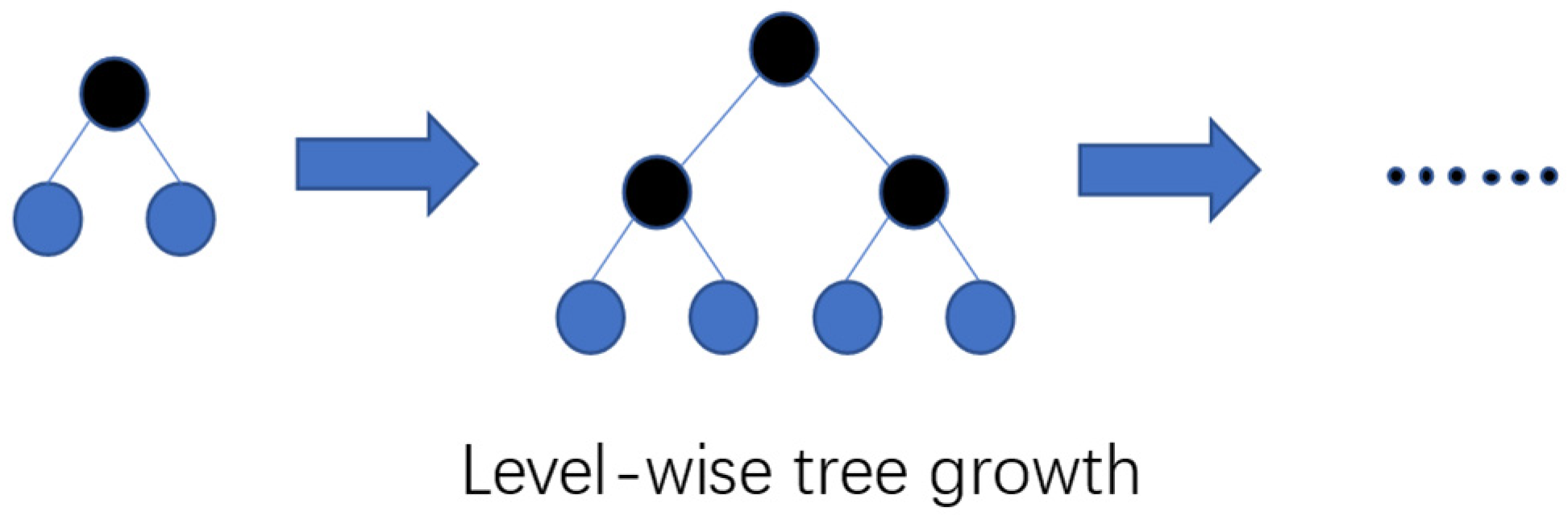
3.1. Introduction to the LightGBM Algorithm

LightGBM is a boosting regression algorithm proposed by Microsoft [38]. It is one of the latest machine learning algorithms also based on decision tree, and the logic about the contributions of each predictor to the final model is the same with the XGB model. It uses the idea of an algorithm based on a histogram to discretize continuous features into several discrete bins. The algorithm based on the histogram avoids calculating all continuous features and takes discrete bins as the unit. This method improves the training efficiency and reduces the memory overhead. In particular, the histogram algorithm also has a subtraction feature, where a target leaf can subtract its neighbor nodes from its parent node. This further accelerates the convergence speed of the algorithm.

In addition to the histogram algorithm (Figure 2), LightGBM adopts the leaf-wise tree growth (Figure 3) strategy and selects the leaf with the largest split gain to grow. Unlike many boosting algorithms that use a level-wise tree growth (Figure 4) strategy, it is a depth-first tree growth strategy. The leaf-wise selects the leaf with the largest split gain to grow, and hence, the depths of different leaf nodes are not the same. Experiments show that the leaf-wise tree growth strategy results in a lower loss. To avoid the over-fitting phenomenon caused by excessive longitudinal growth, LightGBM further sets the maximum depth of the tree.

As an optimized GBDT algorithm, LightGBM has relatively high complexity and is capable of solving nonlinear problems. LightGBM is both efficient and accurate with histogram algorithm, leaf-wise tree growth strategy and other characteristics. The tree model is efficient on the tabular data type used for height prediction of evaporation duct.

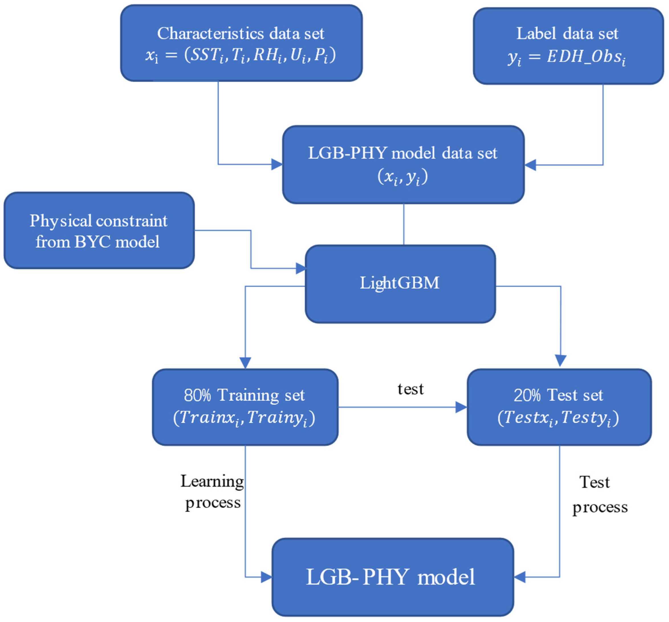
3.2. Construction of LGB-PHY Model

The traditional theoretical model of evaporation duct height incorporates nonlinear factors, such as sea surface temperature, air temperature, relative humidity, wind speed, and atmospheric pressure. For example, the P-J model is a function of sea surface temperature (SST), air temperature (T_a), relative humidity (RH), and wind speed (U), where the function value is the evaporation duct height (EDH):

$$EDH=f(SST,T_a,RH,U,P)$$

(23)

The BYC model is a semi-empirical physical model based on a large number of regional observation experiences and the Monin–Obukhov similarity theory [3]. This model describes the complex physical relationship between the basic meteorological elements and evaporation duct height. This model combines the sea–air flux algorithm of COARE, which has complex physical constraints. After the calculation, we have obtained the contributions of each predictor, 26% from wind speed, 22.3% from air temperature, 21.3% from sea surface temperature, 18.9% from air pressure and 11.5% from relative humidity.

The LightGBM is efficient at dealing with the regression problem of low-dimensional data and can be applied to the low-dimensional observation data sets. The evaporation duct height prediction model based on the LightGBM replaces the traditional theoretical model (which has a large number of physical process descriptions and empirical parameter assumptions) with a machine learning algorithm. This relies on the capability of machine learning algorithms to capture the correlation between data, hence addressing the bottleneck of traditional theoretical models which are limited by physical assumptions and empirical parameters. At the same time, combining the physical formula of the BYC model with the loss function of the LightGBM model imposes certain physical constraints on the process of training and extracting data association. Such constraints lead to a more accurate and scientific machine learning model. Figure 5 shows the way to combine the physical constraints.

The LightGBM evaporation duct height prediction model combining physical information takes the actual observation data as the starting point. Therefore, for the construction of the model the observation data set should be preprocessed first. The sample pair should be set as ${\left(x_i,y_i\right)}^n{}_{i=1}$, and vector $x_{\mathrm{i}}$ expressed as $x_{\mathrm{i}}=\left(SS{T}_i,T_i,R{H}_i,U_i,P_i\right)$ is a five-dimensional vector in which the eigenvalues represent the sea surface temperature, air temperature, relative humidity, wind speed and atmospheric pressure, respectively. Set the measured data as a label $y_i=EDH\_Ob{s}_i$. Here, N is number of samples of which 80% is selected as the training set and the remaining 20% as the test set. Different application areas and data attributes will have different key parameters configuration. According to the specific conditions of the experimental data and some prior knowledge, the parameters are finally determined as follows through a large number of computer experiments: learning rate (learning_rate) = 0.1, number of weak learners (n_estimators) = 4000, number of leaves of the model (num_leaves) = 28, minimum leaf node sample weight (min_child_weight) = 0.001, and minimum leaf node samples (min_child_samples) = 20. The loss function is custom loss function, for training the function name it is custom_normal_train, and for validating the function name it is custom_normal_valid. The key parameters will be fine-tuned according to the amount of data. The flowchart of the model is depicted in Figure 6.

The custom loss function of the model is defined as:

$$Loss=MSE+\alpha MSE\_BYC$$

(24)

As shown in the above formula, the loss function is divided into two parts. The first part is MSE, calculated by the predicted value of evaporation duct height and the tag value, and the second part is MSE_BYC, calculated by the BYC model; the tag value, α, is a weight parameter to ensure that the magnitude balance of the MSE in the two parts. In our experiments, we tried different values of α and found α = 0.01 is an efficient choice.

$$MSE=\frac{1}{n}{\displaystyle \sum _{i=1}^n{(y\_pred-y\_true)}^2}$$

(25)

The above formula is the RMSE obtained from the predicted value and label value of evaporation duct height, where y_pred denotes the predicted value of the model, and y_true represents the true value label of the height of the evaporation duct

$$MSE\_BYC=\frac{1}{n}{\displaystyle \sum _{i=1}^n{(y\_BYC-y\_true)}^2}$$

(26)

The above formula, i.e., MSE_BYC is obtained from the height value and label value of the evaporation duct calculated by the BYC model, where y_BYC refers to the height value of the evaporation duct calculated by the BYC model.

4. Experiment and Result Analysis

4.1. Experimental Scheme

In this study, we obtain the data by deploying observation equipment on the ships, and different data sets correspond to different routes. The ship is equipped with six layers of hydrometeorological fundamental element measuring sensors on the ship deck from low to high and a set of infrared sea surface water temperature sensors. The sensors record the air temperature (°C), relative humidity (%), wind speed (m/s), air pressure (hPa), and SST(°C). For EDH measurement, preprocess the sensor measurement data of the six-layer to refractive index profile, and EDH corresponds to the point with a slope of 0. The method of EDH measurement is improved from Babin’s method [6]. The sensor parameters are shown in

Table 2. The parameters of sensors.

Sensor Category	Range	Precision	Resolution
Air temperature sensor	−40~+70 °C	±0.3 °C	0.1 °C
Relative humidity sensor	0~100%	±2%	1%
Pressure sensor	300~1100 hPa	±0.5 hPa	0.1 hPa
Wind speed sensor	0.1~60 m/s	±3%	0.01 m/s
Sea surface temperature sensor	−55 °C~+80 °C	±0.2 °C	0.1 °C

.

The observation voyage routes have been shown in Figure 7 and the data consists of the following parts:

Part 1: Voyage exploration experiment in the South China Sea (SCS) from 16 November 2020 to 21 November 2020. The corresponding data set is referred to as 5 DaysSCS.

Part 2: Short-distance voyage exploration experiment in the South China Sea. The corresponding data set is called Back, which represents the short-range return data of the South China Sea.

Part 3: Voyage exploration experiment in the Equator. The corresponding data set is referred to as ER.

Part 4: Sailing exploration experiment in the Sea of Sri Lanka. The corresponding data set is called SSL.

Part 5: Navigation exploration experiment in the North Bengal Bay. The corresponding data set is referred to as NBB.

The characteristic values of the above meteorological and hydrological observation data samples are composed of sea surface temperature, air temperature, relative humidity, wind speed at 10 m height on the deck and air pressure. The corresponding EDH values are also collected as the data labels. Eliminating the missing and abnormal data, a total of about 83,000 groups of samples were made available. For the 5 DaySCS data set that includes a large number of samples, the data set was divided into days as a whole. Therefore, the data of the first four days can be used to predict the data of the fifth day. The experiment is divided into two parts. In the first part, 80% of the available data is used as the training set and 20% as the test set to evaluate the comprehensive effect of the LightGBM model. In the second part, the data of four different regions, including Back, ER, SSL and NBB, are used for cross-training. Here, all the data of one region is considered as the training set and the remaining three regions are considered as the test set. The goal is to test the generalization ability of the model area.

The root means square error (RMSE) and R-square (SCC) are also used as performance evaluation indexes. RMSE reflects the accuracy of the model in predicting the height of the evaporation duct. The lower the RMSE value, the higher the prediction accuracy of the model. The SCC represents the goodness of fit between the predicted result and the detected true value. The SCC value is in the range of (0, 1), and a value closer to 1 represents a better goodness of fit, i.e., the higher the degree of explanation of independent variables to dependent variables.

The calculation formulas of RMSE and SCC are as the following

$$RMSE=\sqrt{\frac{1}{n}{\displaystyle \sum _{i=1}^n{(f(x_i)-y_i)}^2}}$$

(27)

$$SCC=\frac{{(n{\displaystyle \sum _{i=1}^{n}f(x_i)y_i-{\displaystyle \sum _{i=1}^{n}f(x_i)y_i{\displaystyle \sum _{i=1}^n{y}_i}}})}^2}{(n{\displaystyle \sum _{i=1}^{n}f{(x_i)}^2-{({\displaystyle \sum _{i=1}^{n}f(x_i)})}^2})(n{\displaystyle \sum _{i=1}^n{y}_i{}^2}-{({\displaystyle \sum _{i=1}^n{y}_i})}^2)}$$

(28)

4.2. Data Augmentation

The 5 DaysSCS data set is a voyage observation data set and many labels are missing in this data set. To make up for this deficiency, we apply data enhancement based on the P-J model, which is the most widely used theoretical model of the evaporation duct. The P-J model has simple principles, a wide application range and provides stable calculated data. The percentage of data coming from data augmentation is 15%. During the observation, because of the observation equipment error and extreme natural conditions [39], sometimes the data label is missing, and the missing data accounts for about 15% of the total data volume. Here, for the data with missing labels, the value of the evaporation duct height model is calculated by using the P-J evaporation duct theoretical model. We then add Gaussian noise [40] to the obtained missing label values calculated by the P-J model to construct enhanced data. This provides samples that closely follow the natural law and meets the research requirements. Additionally, 15% data augmentation makes the data set more diverse on the premise of not reducing the influence of real observation data, the probability of overfitting in the training process is alleviated to some extent.

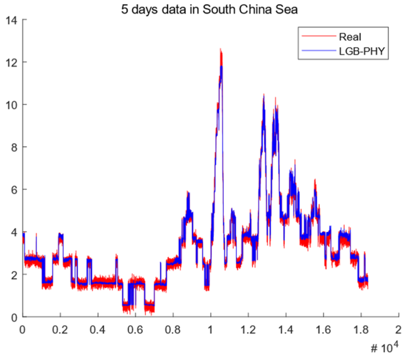
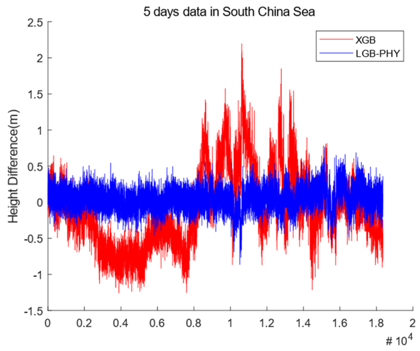
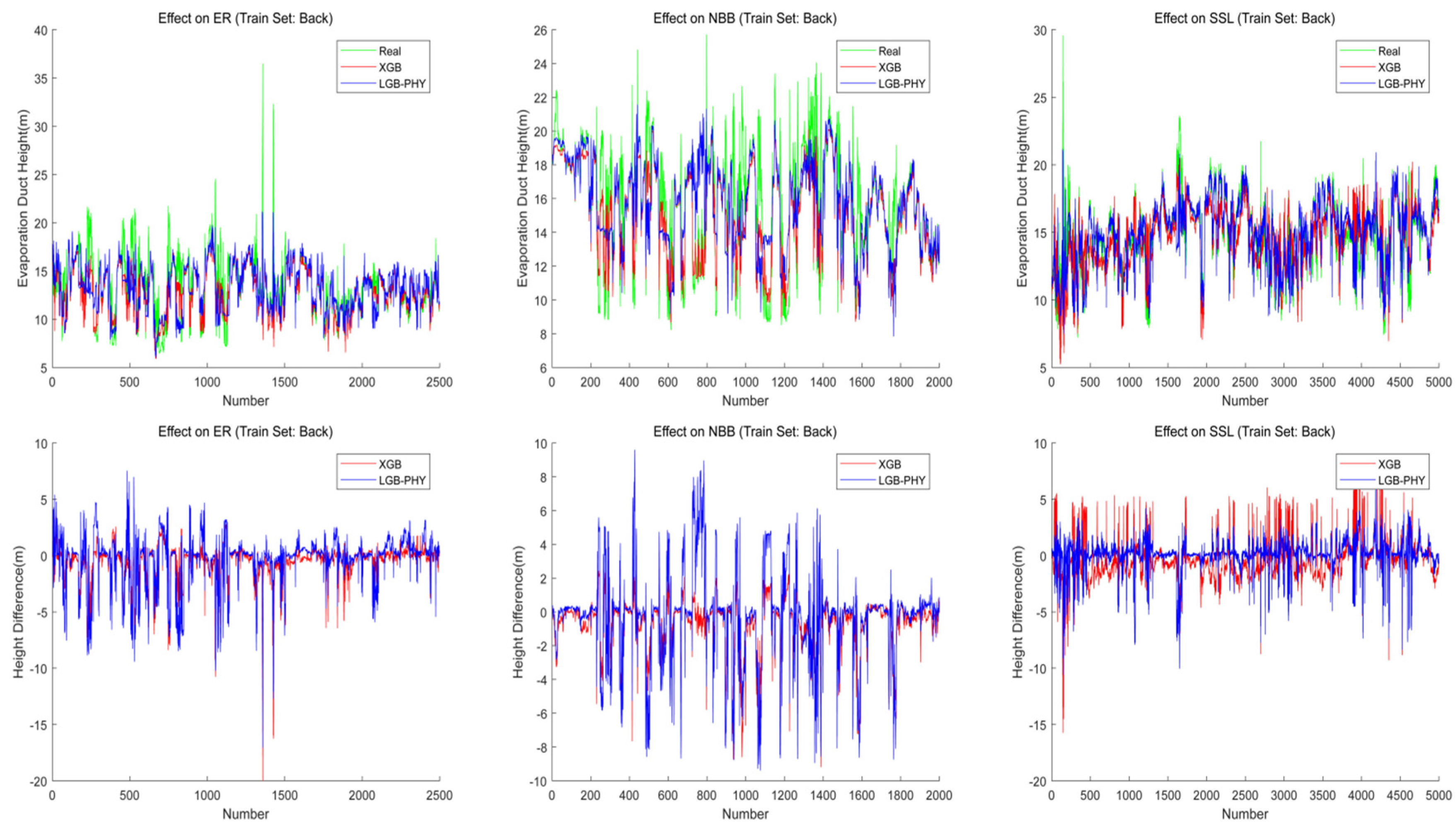
4.3. Evaluation of Model Prediction Effect

To test the prediction effect of the LGB-PHY model, the XGB model driven by pure data and the theoretical BYC model are used as references in the experiment. An 80% of the observed data of 5 DaysSCS obtained from the 5-day South China Sea cruise is also used as the training set, and the remaining 20% is used as the test set for verification. Figure 8 shows the evaporation duct height prediction in the test set which combines the LightGBM model and XGB model. The red line is the real observation value, and the blue line shows the predicted value of evaporation duct height using the LightGBM model with physical information.

It is seen from the above that the predicted value of the evaporation duct by the LightGBM model with physical information closely follows the actual observation value. Figure 8 shows the effectiveness of the new model LightGBM model for the existing data sets.

Figure 9 further shows the difference distribution between the predicted value and the real value of the LGB-PHY and XGB models. The blue line shows the difference distribution between the predicted value and the real value of LGB-PHY, and the red line shows the difference distribution between the predicted value and the real value of the XGB model. It is seen that the LGB-PHY model provides better fitting performance of real values.

Table 3. The RMSE and SCC values of LGB-PHY and XGB models.

	RMSE	SCC
LGB-PHY	0.166	0.993
XGB	0.512	0.932

shows the RMSE and SCC values of the LGB-PHY and XGB models.

As is seen in Table 3, LGB-PHY model overperforms the XGB both in terms of RMSE and SCC.

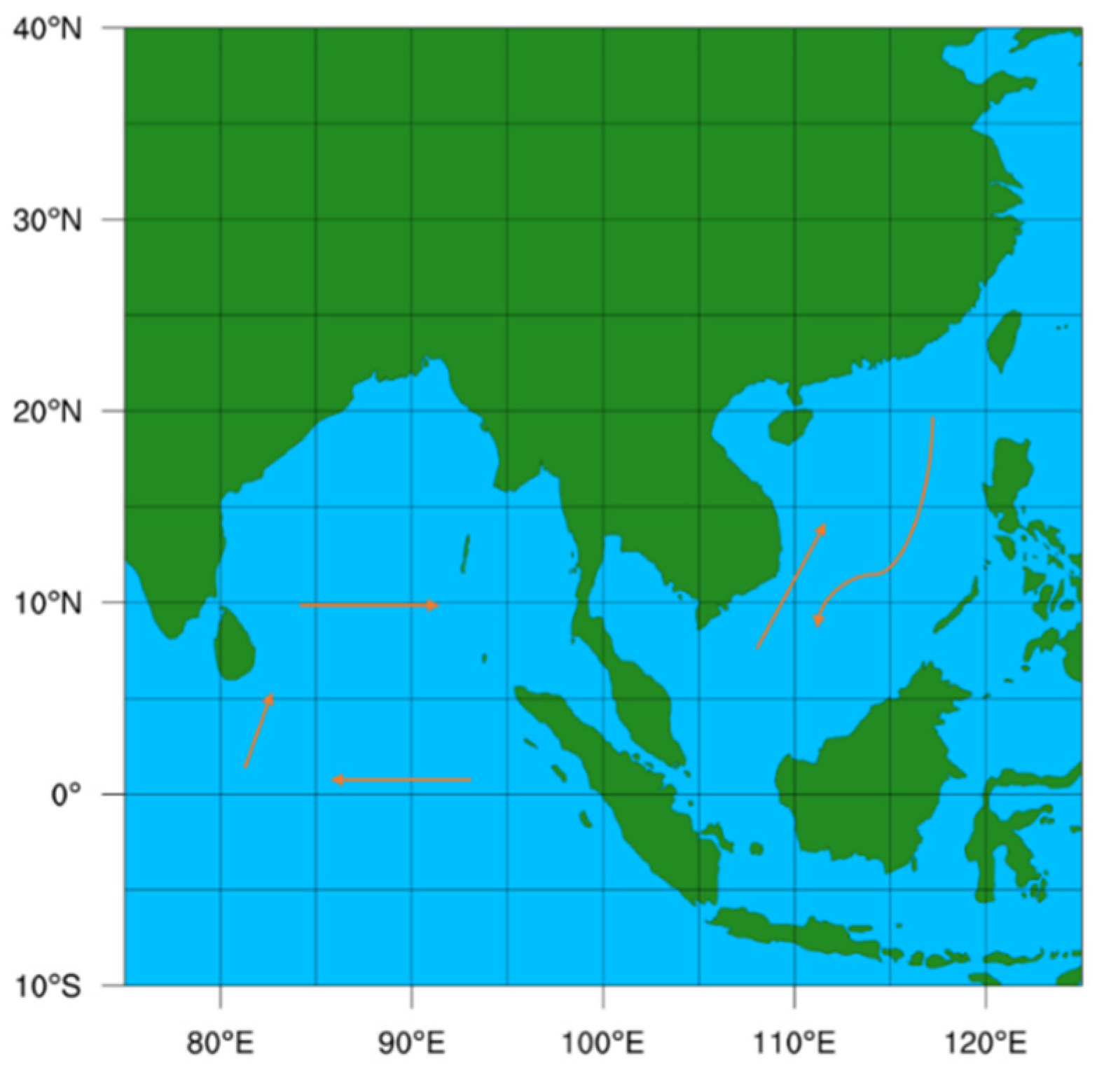
4.4. Model Area Generalization Ability Test

To investigate the performance of the generalization ability, a sub-region data of each observed data set is used as the training set, and the rest of the sub-region data are used as the test set. The XGB model and LGB-PHY model are then compared in different combinations of experimental areas. This experiment shows that the LGB-PHY model overperforms the XGB model in terms of regional generalization.

Back, NBB, SSL, and ER data sets in four different regions, and all of the sub-data sets, are used as the training set each time. The trained model is then tested in the remaining four regions, and the prediction results are shown in Figure 10, where the blue line indicates the output result predicted by the LGB-PHY model combining physical information, and the red line indicates the output result predicted by XGB model. The green line also indicates the observation value of the evaporation duct height in this area.

The plots in Figure 10 show the comparison between the predicted value and the real value of the model using Back data as the training set and the data of the other three areas as the test set. The plots below also present the difference between the output value of the two models and the true value.

The plots above in Figure 11 demonstrate the comparison between the predicted value and the real value of the model using ER data set as the training set and the data of the other four areas as the test set. The plots below in Figure 11 also indicate the difference between the output value of the two models and the true value.

The plots above in Figure 12 indicate the comparison between the predicted value and the real value of the model using NBB data as the training set and the data of the other four regions as the test set. The plots below in Figure 12 show the difference between the output value of the two models and the true value.

In Figure 13, we also present the comparison between the predicted value and the real value of the model using SSL data as the training set and the data of the other four areas as the test set. The plots below in Figure 13 demonstrate shows the difference between the output value of the two models and the true value.

The model performance differs among regions because the different data sets from different regions have different data characteristics. The machine learning models are pure data-driven evaporation duct models. The LightGBM algorithm and the physical constraints give the model a better ability to extract features of data and fit the true observation value of the evaporation duct height.

The data sets of different regions are from the observative experiment in different regions. Influenced by different meteorological and hydrological conditions in different regions, the different data sets from different areas have different data characteristics, and the different data characteristics affect the feature extraction of the model and the fitting effect of the true value.

Table 4. The RMSE values of LGB-PHY model in model area generalization ability test.

	Train Area	SSL	NBB	Back	ER
LGB-PHY (RMSE)	SSL	-	2.41	1.30	1.40
	NBB	1.49	-	0.89	1.18
	Back	1.47	2.75	-	2.39
	ER	1.03	1.04	1.17	-

,

Table 5. The RMSE values of XGB model in model area generalization ability test.

	Train Area	SSL	NBB	Back	ER
XGB (RMSE)	SSL	-	2.46	1.04	1.20
	NBB	1.95	-	0.92	1.48
	Back	1.84	1.91	-	1.90
	ER	1.44	1.07	1.35	-

,

Table 6. The SCC values of LGB-PHY model in model area generalization ability test.

	Train Area	SSL	NBB	Back	ER
LGB-PHY (SCC)	SSL	-	0.47	0.82	0.77
	NBB	0.65	-	0.92	0.84
	Back	0.66	0.31	-	0.34
	ER	0.83	0.90	0.86	-

and

Table 7. The SCC values of the XGB model in model area generalization ability test.

	Train Area	SSL	NBB	Back	ER
XGB (SCC)	SSL	-	0.44	0.88	0.83
	NBB	0.39	-	0.91	0.75
	Back	0.46	0.66	-	0.58
	ER	0.67	0.89	0.81	-

show the root mean square error (RMSE) and R-square (SCC) values of different models under different experimental conditions.

Based on the above results, the following observations are made:

(1)

In most cases, the RMSE of the predicted value of the LGB-PHY model is smaller than that of the XGB model, and the SCC of the predicted value of the LGB-PHY model is larger than that of the XGB model. Hence, the LGB-PHY model has better generalization performance in most cases.

(2)

In cases where the SSL data set is used as the training set, the RMSE of the LGB-PHY model is slightly larger than that of the XGB model where Back and ER are used as test sets, and SCC is slightly smaller than that of the XGB model. In cases where the Back data set is used as the training set, the RMSE of the LGB-PHY model is larger than that of the XGB model when NBB and ER are used as the test sets, and SCC is also smaller than that of the XGB model. According to the adaptability analysis of the BYC theoretical model, it can then be argued that the reason for the errors in some sea areas is that the LGB-PHY model, which combines the physical information of the BYC model, also inherits some of the properties of the BYC theoretical model. Note that there are empirical parameters from the actual observation in the BYC model (i.e., the data of the extracted empirical parameters come from the meteorological and hydrological data observed by the U.S. Navy in the middle and high latitudes) which are significantly different from the air and sea environments in the low latitudes around the equator. It is difficult for the BYC model to achieve good results in the waters near the equator, which leads to the error in some areas of the LGB-PHY model as it combines the physical information of the BYC model.

5. Conclusions

Influenced by the physical parameters that are not universal, the traditional evaporation duct theoretical models have limited accuracy and poor generalization ability. In this study, we address these issues by proposing the physically constrained LightGBM evaporation duct height prediction model (LGB-PHY). By comparing this model with the existing pure data-driven XGB evaporation duct height prediction model, the following conclusions are drawn:

(1)

In the South China Sea, the LGB-PHY model has higher fitting accuracy than the XGB model. The experiments performed that the LGB-PHY model has higher performance in terms of RMSE and SCC than that of the XGBM model, where the RMSE index decreases by 68% and the SCC index increases by 6.5%.

(2)

In the cross-comparison experiment of regional generalization, the LGB-PHY model shows better generalization ability than that of the XGB model in most cases. Nevertheless, for the case with the Back data set as the training set and the NBB data set being used as the test set, the LGB-PHY model demonstrates lower. It is attributed to the fact that some empirical parameters in the BYC model are derived from actual observation. However, the observation site is situated where the empirical parameters are mostly located in the sea area of the middle and high latitudes, which are quite different from the atmosphere and sea environment of the low latitudes around the equator. Affected by the poor universality of the physical experience parameters, the BYC model has difficulty achieving good results in the waters near the equator and at low latitudes. This results in lower accuracy of the LGB-PHY model, which combines the physical information of the BYC model. In general, our experiments confirm that in the middle and high latitudes, where the BYC model has strong adaptability, the LGB-PHY model has a stronger regional generalization performance.

Compared with the previous pure data-driven model based on machine learning, the proposed LGB-PHY model, which combines physical conditions, improves the accuracy and generalization ability. This model also inherits the characteristics of the theoretical model, hence being physically explainable. The proposed method constitutes a novel technique integrating physical constraints into machine learning methods.

References

1. Kang, S.F.; Zhang, Y.S. Atmospheric Duct in Troposphere Environment; Wang, Z., Ed.; Science Press: Beijing, China, 2014. [Google Scholar]
2. Paulus, R.A. Practical Application of an Evaporation Duct Model. Radio Sci. 1985, 20, 887–896. [Google Scholar] [CrossRef]
3. Jeske, H. State and Limits of Prediction Methods of Radar Wave Propagation Conditions Over Sea. Modern Radio Wave Propagation and Air-Sea interaction. 1973, 5, 130–148. [Google Scholar]
4. Xie, L.X.; Tian, B. Study on Evaporation Duct RSHMU Model in Tropical Waters. Ship Electron. Eng. 2015, 35, 88–90, 100. [Google Scholar]
5. Luc, M.G.; Sylvie, G.; Eric, B. A Simple Method to Determine Evaporation Duct Height in the Sea Surface Boundary Layer. Radio Sci. 1992, 27, 635–644. [Google Scholar]
6. Steven, M.B.; George, S.Y.; James, A.C. A New Model of the Oceanic Evaporation Duct. J. Appl. Meteorol. 1997, 36, 193–204. [Google Scholar]
7. Frederickson, P.A. Estimating the Refractive Index Structure Parameter (C2) over the Ocean Using Bulk Methods. J. Appl. Meteorol. 2000, 39, 10. [Google Scholar]
8. Liu, C.G.; Huang, J.Y. Modeling Evaporation Duct over Sea with Pseudo-Refractivity and Similarity Theory. Acta Electron. Sin. 2001, 29, 970–972. [Google Scholar]
9. Dai, F.S.; Li, Q. Atmospheric Duct and Its Military Applications; People’s Liberation Army Publishing House: Beijing, China, 2002. [Google Scholar]
10. Ding, J.L.; Fei, J.F. Development and validation of an evaporation duct model. part i: Model establishment and sensitivity experiments. J. Meteorol. Res. 2015, 29, 467–481. [Google Scholar] [CrossRef]
11. Song, W.; Tian, B. Research on evaporation duct predicting model. J. Huazhong Univ. Sci. Technol. 2013, 41, 52–56. [Google Scholar]
12. Gerstoft, P.; Rogers, L.T. Inversion for refractivity parameters from radar sea clutter. Radio Sci. 2003, 38, 1–22. [Google Scholar] [CrossRef]
13. Yardim, C.; Gerstoft, P. Sensitivity analysis and performance estimation of refractivity from clutter techniques. Radio Sci. 2009, 44, 1008. [Google Scholar] [CrossRef]
14. Tian, S.S.; Cai, H. Erected antenna height of radars for searching over sea under evaporation duct. J. Huazhong Univ. Sci. Technol. 2010, 38, 16–19. [Google Scholar]
15. Zhang, J.P.; Wu, Z.S. Evaporation duct inversion based on radar sea clutters from different antenna heights. Chin. J. Radio Sci. 2011, 26, 422–430. [Google Scholar]
16. Zhao, X.; Huang, S. Atmospheric Duct Estimation Using Radar Sea Clutter Returns by the Adjoint Method with Regularization Technique. J. Atmos. Ocean. Technol. 2014, 31, 1250–1262. [Google Scholar] [CrossRef]
17. Wang, H.G.; Wu, Z.S. Retrieving evaporation duct heights from power of ground-based GPS occultation Signal. Prog. Electromagn. Res. 2013, 30, 189–194. [Google Scholar] [CrossRef] [Green Version]
18. Anderson, J.R.; Michalski, R.S.; Mitchell, T.M. Machine learning. An Artificial Intelligence Approach; Morgan Kaufmann Publishers Inc.: San Francisco, CA, USA, 1983; Volume 2. [Google Scholar]
19. Isaakids, S.; Dimou, I.; Xenos, T. An artificial neural network predictor for tropospheric surface duct phenomena. Nonlinear Processes Geophys. 2007, 14, 569–573. [Google Scholar] [CrossRef]
20. Douvenot, R.; Fabbro, V.; Bourlier, C. Radar coverage prediction over ocean: Duct mapping using least squares support vector machines. In Proceedings of the 1st European Conference on Antennas and Propagation, Nice, France, 1 June 2006. [Google Scholar]
21. Yang, C. A comparison of the machine learning algorithm for evaporation duct Estimation. Radioengineering 2013, 22, 657–661. [Google Scholar]
22. Zhu, X.Y.; Li, J.C. An Evaporation Duct Height Prediction Method Based on Deep Learning. IEEE Geosci. Remote Sens. Lett. 2018, 15, 1307–1311. [Google Scholar] [CrossRef]
23. Zhu, X.Y.; Zhu, M. An Optimization Research of Evaporation Duct Prediction Models Based on a Deep Learning Method. In Proceedings of the 2018 2nd IEEE Advanced Information Management, Communicates, Electronic and Automation Control Conference, Xi’an, China, 25–27 May 2018. [Google Scholar]
24. Allan, P. Approximation theory of the MLP model in neural networks. Acta Numer. 1999, 8, 143–195. [Google Scholar]
25. Zhao, W.P.; Li, J.C. Research on Evaporation Duct Height Prediction Based on Back Propagation Neural Network. IET Microw. Antennas Propag. Inst. Eng. Technol. 2020, 14, 1547–1554. [Google Scholar] [CrossRef]
26. Zhao, W.P.; Li, J.C. PDD_GBR: Research on Evaporation Duct Height Prediction Based on Gradient Boosting Regression Algorithm. Radio Sci. 2019, 54, 949–962. [Google Scholar] [CrossRef]
27. Zhao, W.P.; Li, J. XGB Model: Research on Evaporation Duct Height Prediction Based on XGBoost Algorithm. Radioengineering 2020, 29, 81–93. [Google Scholar] [CrossRef]
28. Anghel, A.; Papandreou, N. Benchmarking and Optimization of Gradient Boosted Decision Tree Algorithms. Statistics 2018, 2, 1467–1531. [Google Scholar]
29. Jie, H.; Jia, J.W. Evaporation Duct Height Nowcasting in China’s Yellow Sea Based on Deep Learning. Remote Sens. 2021, 13, 1577. [Google Scholar]
30. Steven, M.B. LKB-based evaporation duct model comparison with buoy data. J. Appl. Meteorol. 2002, 41, 434–446. [Google Scholar]
31. Liu, W.T.; Blanc, T.V. The Liu, Katsaros, and Businger (1979) Bulk Atmospheric Flux Computational Iteration Program in FOR-Tran and Basic; Naval Research Lab: Washington, DC, USA, 1984. [Google Scholar]
32. Cook, J.A. A sensitivity study of weather data inaccuracies on evaporation duct height algorithms. Radio Sci. 2016, 26, 731–746. [Google Scholar] [CrossRef]
33. Breiman, L. Stacked Regressions. Mach. Learn. 1996, 24, 49–64. [Google Scholar] [CrossRef] [Green Version]
34. Mitchell, T. Machine Learning and Data Mining. Commun. ACM 1999, 42, 30–36. [Google Scholar] [CrossRef]
35. Jerome, H.F. Greedy function approximation: A gradient boosting machine. Ann. Stat. 2001, 29, 1187–1232. [Google Scholar]
36. Chen, T.; Carlos, C. XGBoost: A Scalable Tree Boosting System. In Proceedings of the KDD ’16: The 22nd ACM SIGKDD International Conference on Knowledge Discovery and Data Mining, San Francisco, CA, USA, 13–17 August 2016. [Google Scholar]
37. Shi, H. Best-First Decision Tree Learning; University of Waikato: Hamilton, New Zealand, 2007. [Google Scholar]
38. Meng, Q. LightGBM: A Highly Efficient Gradient Boosting Decision Tree. In Proceedings of the Advances in Neural Information Processing Systems 30 (NIPS 2017), Long Beach, CA, USA, 4–9 December 2017; Volume 30. [Google Scholar]
39. Paulson, A.C. The Mathematical Representation of Wind Speed and Temperature Profiles in the Unstable Atmospheric Surface Layer. J. Appl. Meteorol. 1970, 9, 857–861. [Google Scholar] [CrossRef]
40. Hilarie, S.; Christopher, J. Gaussian Process Regression for Estimating EM Ducting Within the Marine Atmospheric Boundary Layer. Radio Sci. 2020, 55, 1–14. [Google Scholar]
Figure 1. A radar blind zone caused by the atmospheric duct.
Remotesensing 14 03448 g001
Figure 2. The histogram algorithm.
Remotesensing 14 03448 g002
Figure 3. The leaf-wise algorithm.
Remotesensing 14 03448 g003
Figure 4. The level-wise algorithm.
Remotesensing 14 03448 g004
Figure 5. Combining the physical constraints.
Remotesensing 14 03448 g005
Figure 6. The model structure diagram.
Remotesensing 14 03448 g006
Figure 7. The voyage routes.
Remotesensing 14 03448 g007
Figure 8. The fitting effect of LGB-PHY.
Remotesensing 14 03448 g008
Figure 9. The difference distribution between the predicted and real values of the LGB-PHY and XGB models.
Remotesensing 14 03448 g009
Figure 10. Comparison between the predicted value and the real value of the model using Back data as the training set and the data of the other three areas as the test set.
Remotesensing 14 03448 g010
Figure 11. The comparison between the predicted and real values of the model using ER data as the training set and the data of the other three areas as the test set.
Remotesensing 14 03448 g011
Figure 12. The comparison between the predicted and real values of the model using NBB data as the training set and the data of the other three areas as the test set.
Remotesensing 14 03448 g012
Figure 13. Comparison between the predicted value and the real value of the model using SSL data as the training set and the data of the other three areas as the test set.
Remotesensing 14 03448 g013