
Remote Sensing Application for Landslide Detection, Monitoring along Eastern Lake Michigan (Miami Park, MI)

 ,
,  , and
, and 
Abstract
:
1. Introduction
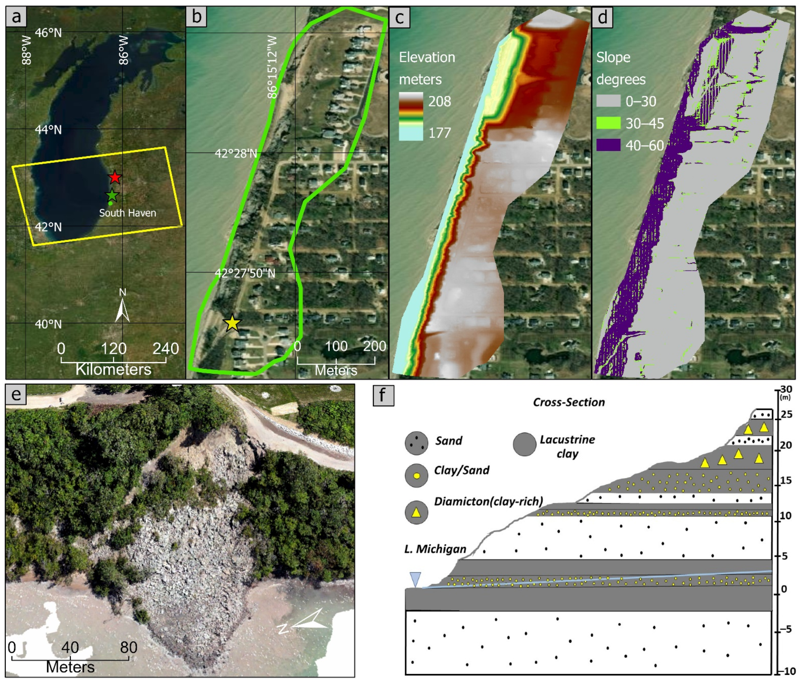
2. Study Area
3. Data and Methodology
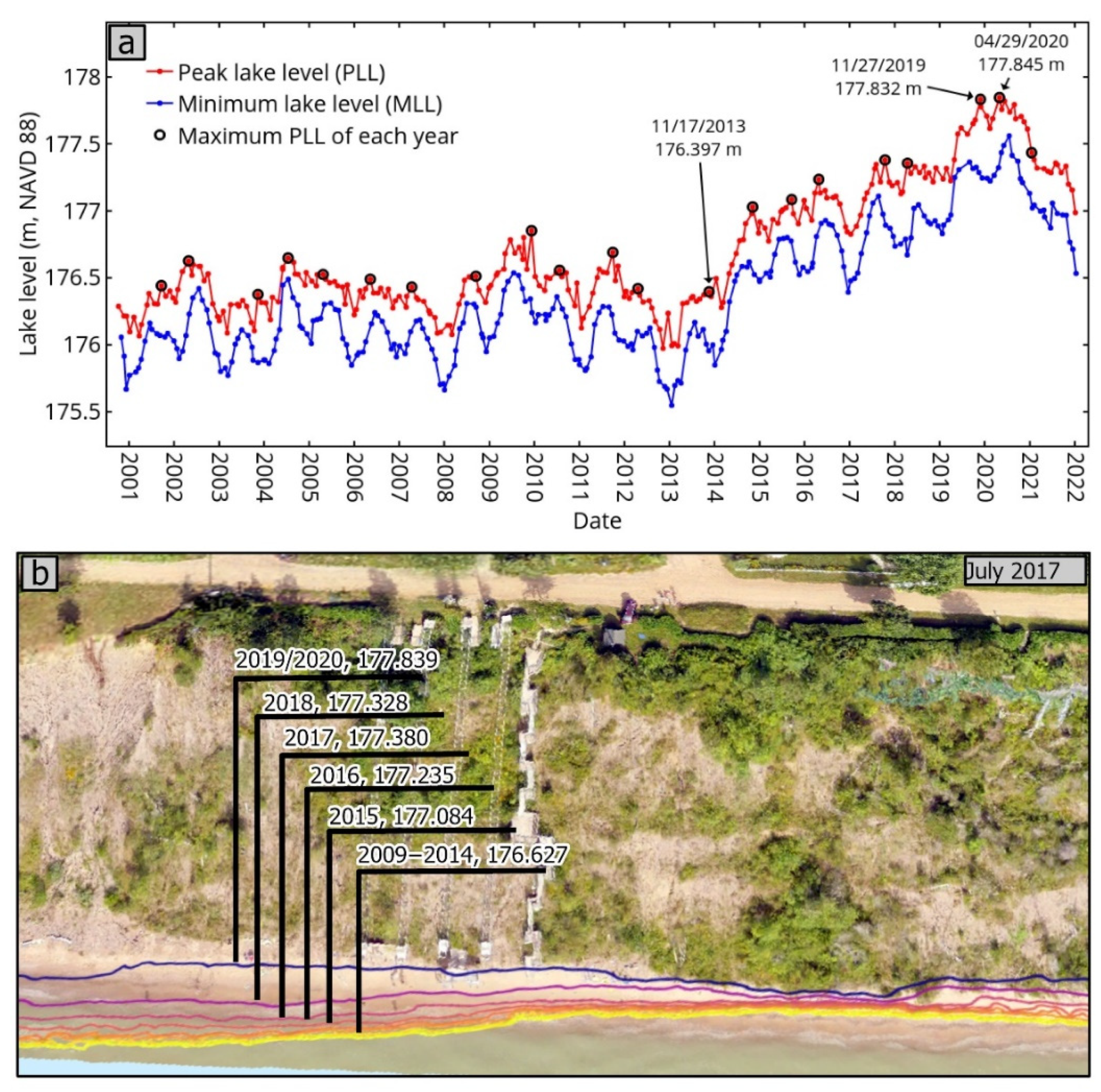
3.1. Lake Level
3.2. UAV Data and Processing
3.3. SAR Data
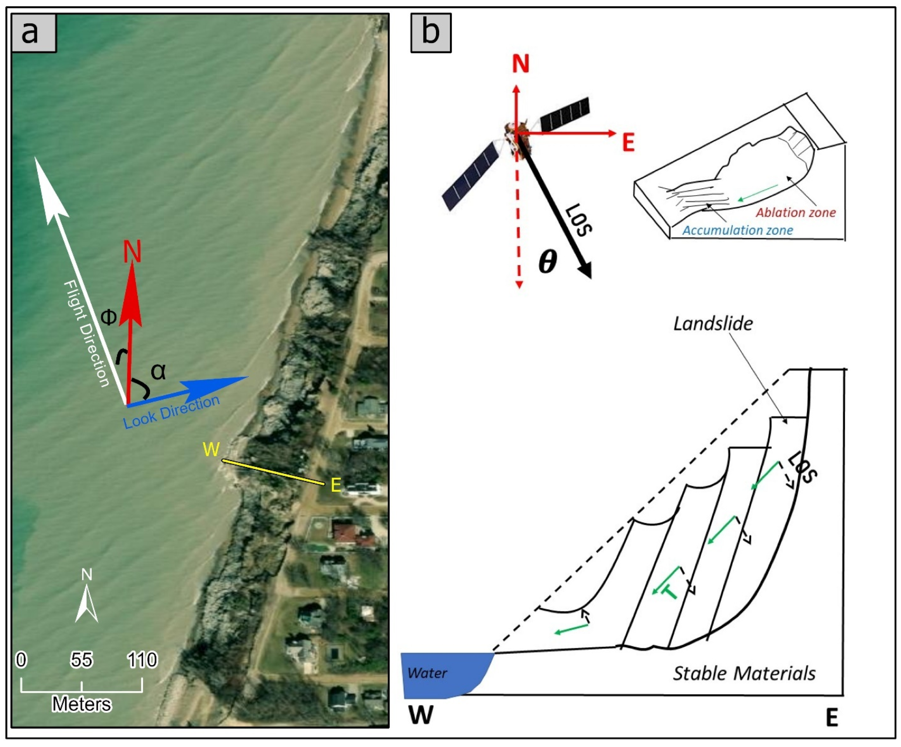
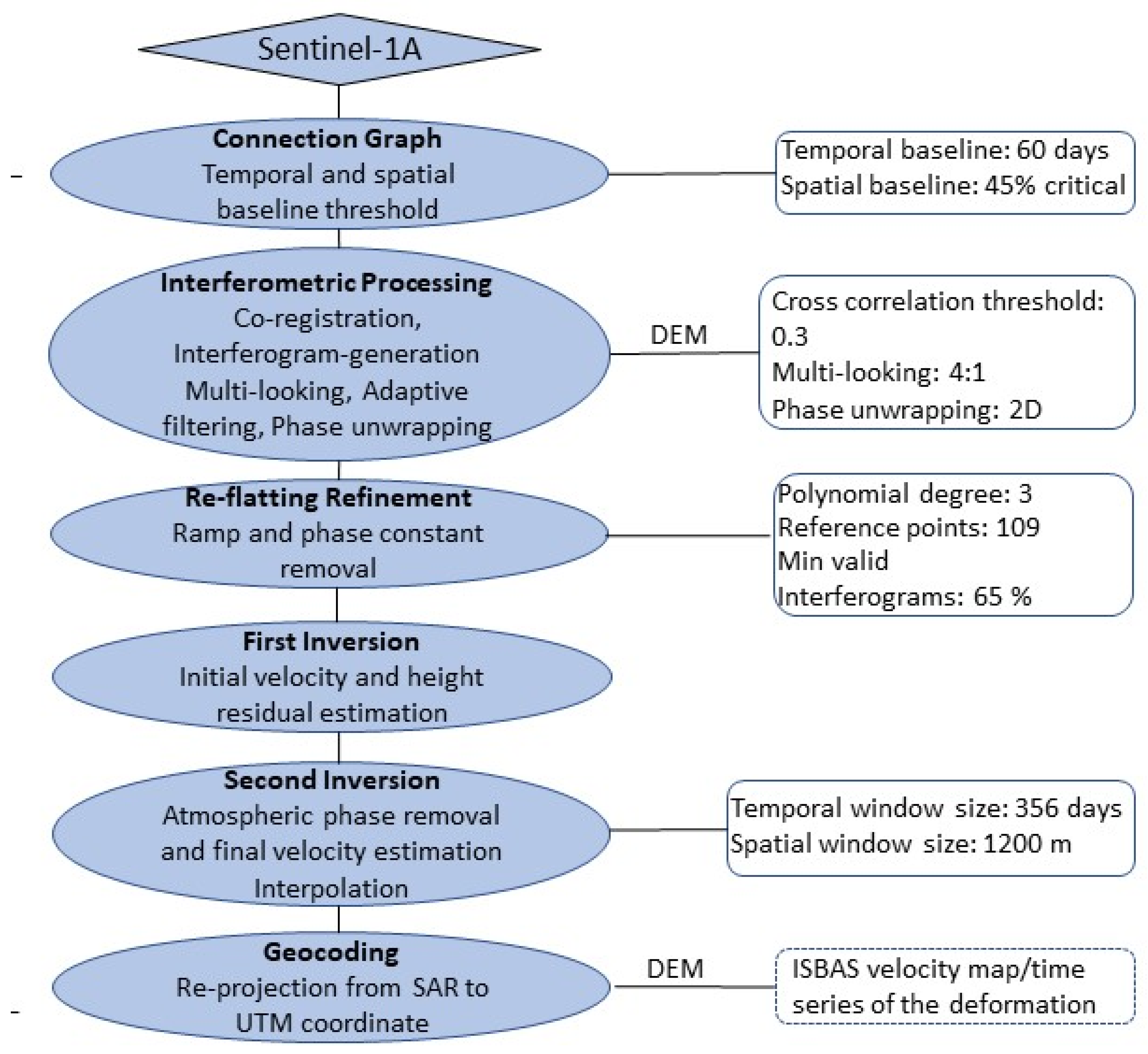
3.4. InSAR Methodology
4. Results
4.1. Refinement of SBAS Application
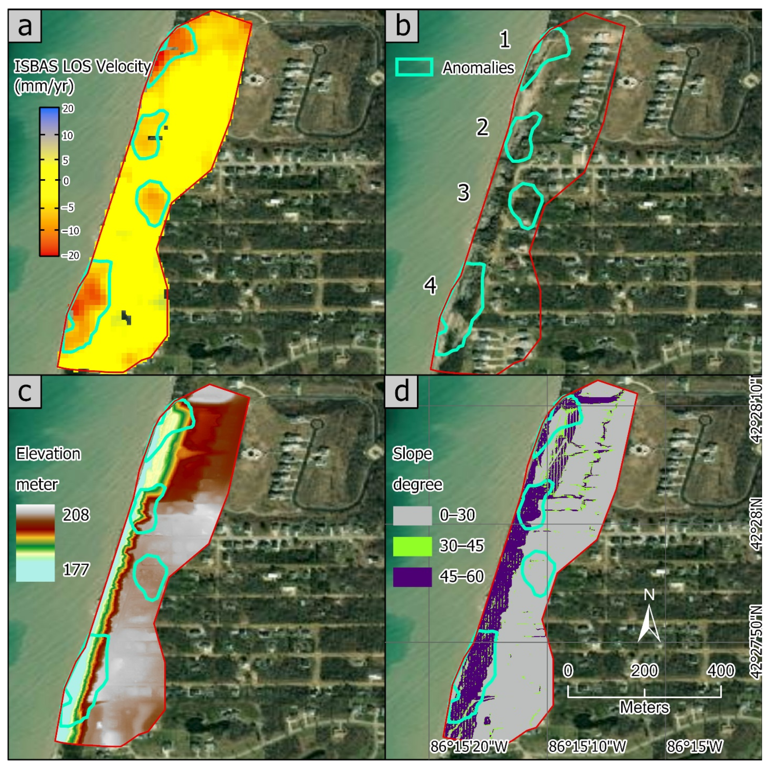
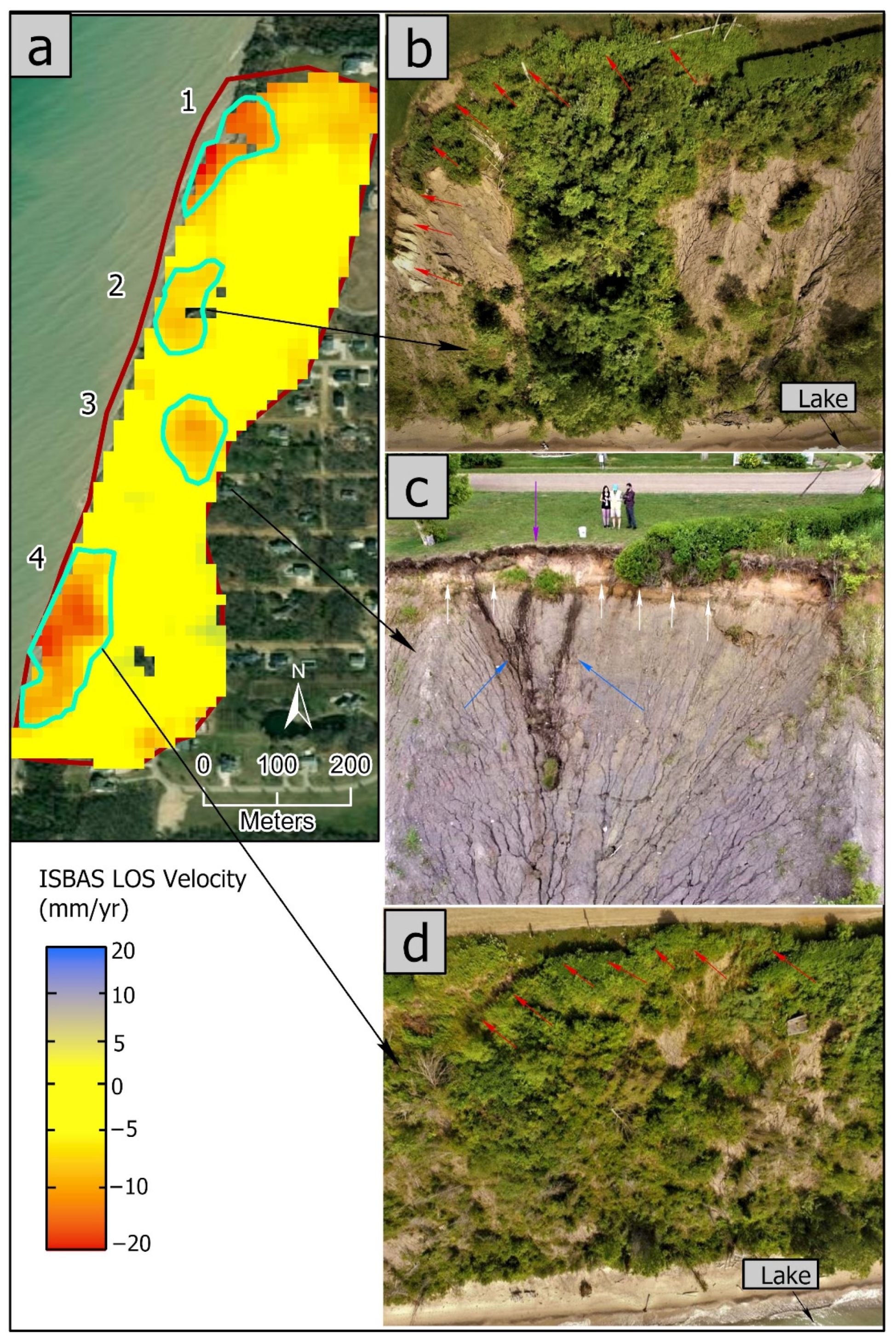
4.2. Slow Deformation, Spatial and Temporal Distribution, Controlling Factors
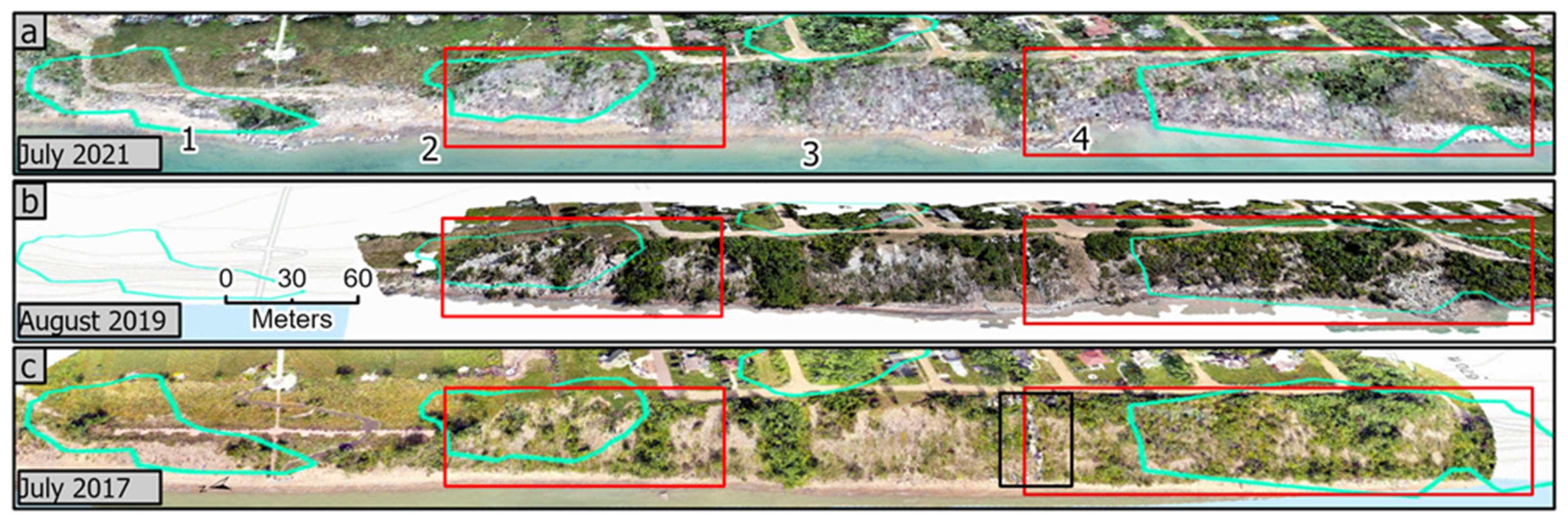
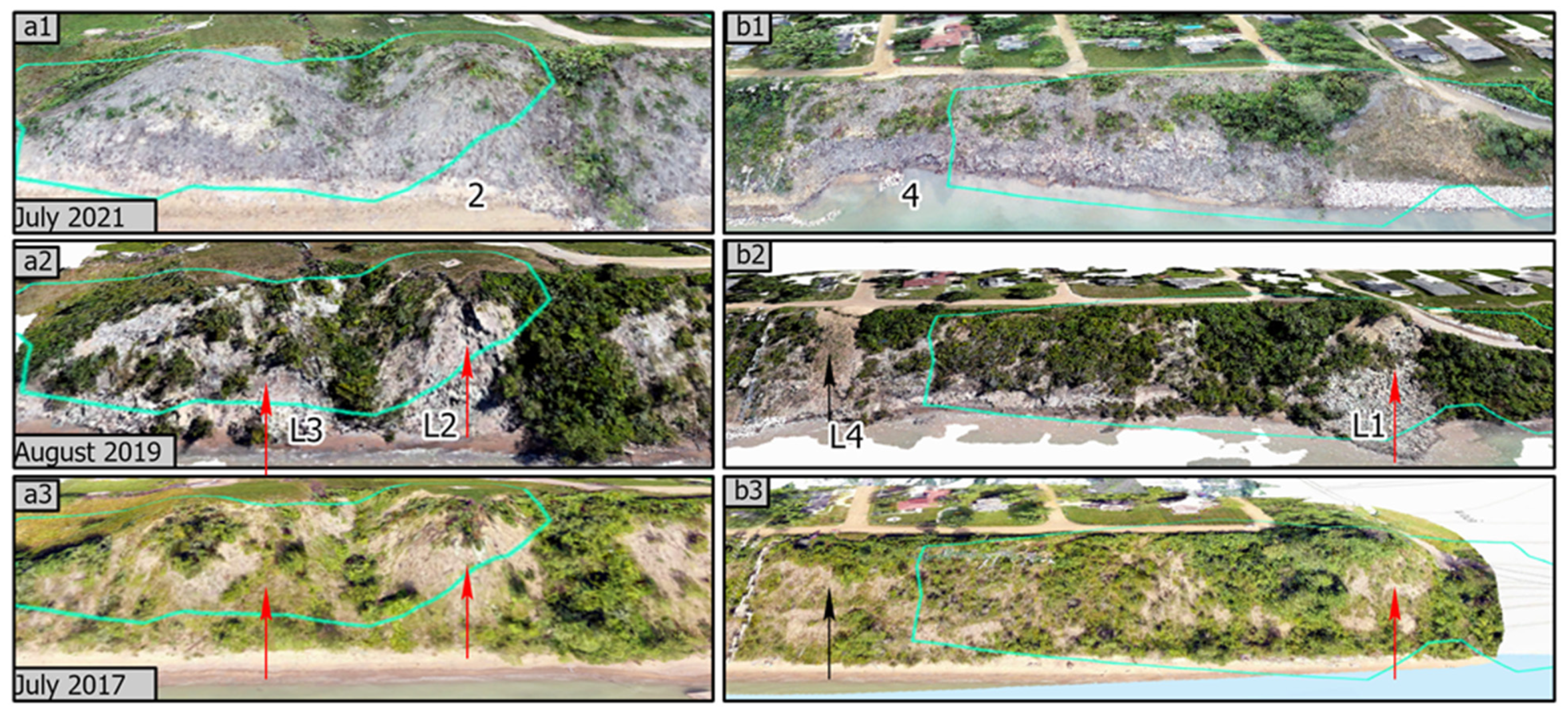
4.3. Rapid Deformation: Spatial and Temporal Distribution
5. Discussion
6. Conclusions
Author Contributions
Funding
Data Availability Statement
Acknowledgments
Conflicts of Interest
References
- Volpano, C.A.; Zoet, L.K.; Rawling, J.E.; Theuerkauf, E.J.; Krueger, R. Three-Dimensional Bluff Evolution in Response to Seasonal Fluctuations in Great Lakes Water Levels. J. Great Lakes Res. 2020, 46, 1533–1543. [Google Scholar] [CrossRef]
- Swenson, M.J.; Wu, C.H.; Edil, T.B.; Mickelson, D.M. Bluff Recession Rates and Wave Impact along the Wisconsin Coast of Lake Superior. J. Great Lakes Res. 2006, 32, 512–530. [Google Scholar] [CrossRef] [Green Version]
- Jibson, R.W.; Odum, J.K.; Staude, J.M. Rates and Processes of Bluff Recession Along the Lake Michigan Shoreline in Illinois. J. Great Lakes Res. 1994, 20, 135–152. [Google Scholar] [CrossRef]
- Lawrence, P.L. Natural Hazards of Shoreline Bluff Erosion: A Case Study of Horizon View, Lake Huron. Geomorphology 1994, 10, 65–81. [Google Scholar] [CrossRef]
- Castedo, R.; Fernández, M.; Trenhaile, A.S.; Paredes, C. Modeling Cyclic Recession of Cohesive Clay Coasts: Effects of Wave Erosion and Bluff Stability. Mar. Geol. 2013, 335, 162–176. [Google Scholar] [CrossRef]
- Meadows, G.A.; Meadows, L.A.; Wood, W.L.; Hubertz, J.M.; Perlin, M. The Relationship between Great Lakes Water Levels, Wave Energies, and Shoreline Damage. Bull. Am. Meteorol. Soc. 1997, 78, 675–683. [Google Scholar] [CrossRef] [Green Version]
- Gronewold, A.D.; Fortin, V.; Lofgren, B.; Clites, A.; Stow, C.A.; Quinn, F. Coasts, Water Levels, and Climate Change: A Great Lakes Perspective. Clim. Change 2013, 120, 697–711. [Google Scholar] [CrossRef]
- Edil, T.B.; Vallejo, L.E. Mechanics of Coastal Landslides and the Influence of Slope Parameters. Eng. Geol. 1980, 16, 83–96. [Google Scholar] [CrossRef]
- Meadows, G.A.; Grimm, A.; Brooks, C.N. Remote Sensing-Based Detection and Monitoring of Dangerous Nearshore Currents. In Proceedings of the IAGLR 58th Annual Conference on Great Lakes Research, University of Vermont, Burlington, VT, USA, 25–29 May 2015; Michigan Tech Research Institute Publications: Ann Arbor, MI, USA, 2015. [Google Scholar]
- Krueger, R.; Zoet, L.K.; Rawling, J.E. Coastal Bluff Evolution in Response to a Rapid Rise in Surface Water Level. J. Geophys. Res. Earth Surf. 2020, 125, e2019JF005428. [Google Scholar] [CrossRef]
- Brown, E.A.; Wu, C.H.; Mickelson, D.M.; Edil, T.B. Factors Controlling Rates of Bluff Recession at Two Sites on Lake Michigan. J. Great Lakes Res. 2005, 31, 306–321. [Google Scholar] [CrossRef] [Green Version]
- Montgomery, W.W. Groundwater Hydraulics and Slope Stability Analysis: Elements for Prediction of Shoreline Recession. Ph.D. Thesis, Western Michigan University, Kalamazoo, MI, USA, 1998. Available online: https://scholarworks.wmich.edu/dissertations/1583 (accessed on 25 May 2022).
- Friele, P.; Millard, T.H.; Mitchell, A.; Allstadt, K.E.; Menounos, B.; Geertsema, M.; Clague, J.J. Observations on the May 2019 Joffre Peak Landslides, British Columbia. Landslides 2020, 17, 913–930. [Google Scholar] [CrossRef] [Green Version]
- Lantz, T.C.; Kokelj, S.V. Increasing Rates of Retrogressive Thaw Slump Activity in the Mackenzie Delta Region, N.W.T., Canada. Geophys. Res. Lett. 2008, 35, L06502. [Google Scholar] [CrossRef]
- Glynn, M.E.; Chase, R.B.; Kehew, A.E.; Selegean, J.P.; Ferrick, M.G.; Hansen, C.M. Lake Michigan Bluff Dewatering and Stabilization Study—Allegan County, Michigan; U.S. Army Corps of Engineers: Washington, DC, USA, 2012.
- Kaufmann, V. Mapping of the 3D Surface Motion Field of Doesen Rock Glacier (Ankogel Group, Austria) and Its Spatio-Temporal Change (1954-1998) by Means of Digital Photogrammetry. In Proceedings of the 7th International Conference on Permafrost, Yellowknife, Canada, 23–27 June 1998; pp. 551–556. [Google Scholar]
- Eriksen, H.Ø.; Lauknes, T.R.; Larsen, Y.; Corner, G.D.; Bergh, S.G.; Dehls, J.; Kierulf, H.P. Visualizing and Interpreting Surface Displacement Patterns on Unstable Slopes Using Multi-Geometry Satellite SAR Interferometry (2D InSAR). Remote Sens. Environ. 2017, 191, 297–312. [Google Scholar] [CrossRef] [Green Version]
- Kaunda, R.B.; Chase, R.B.; Kehew, A.E.; Kaugars, K.; Selegean, J.P. Interpretation of a Progressive Slope Movement Using Balanced Cross Sections and Numerical Integration. Environ. Eng. Geosci. 2008, 14, 121–131. [Google Scholar] [CrossRef]
- Chase, R.B.; Kehew, A.E.; Glynn, M.E.; Selegean, J.P. Modeling Debris Slide Geometry with Balanced Cross Sections: A Rigorous Field Test. Environ. Eng. Geosci. 2007, 13, 45–53. [Google Scholar] [CrossRef]
- Zoet, L.K.; Rawling, J.E. Analysis of a Sudden Bluff Failure along the Southwest Lake Michigan Shoreline. J. Great Lakes Res. 2017, 43, 999–1004. [Google Scholar] [CrossRef]
- Konrad, S.K.; Humphrey, N.F.; Steig, E.J.; Clark, D.H.; Potter, N.; Pfeffer, W.T. Rock Glacier Dynamics and Paleoclimatic Implications. Geology 1999, 27, 1131–1134. [Google Scholar] [CrossRef]
- Krainer, K.; He, X. Flow Velocities of Active Rock Glaciers in the Austrian Alps. Geogr. Ann. Ser. A Phys. Geogr. 2006, 88, 267–280. [Google Scholar] [CrossRef]
- Bauer, A.; Paar, G.; Kaufmann, V. Terrestrial Laser Scanning for Rock Glacier Monitoring. In Proceedings of the 8th International Conference on Permafrost, Zurich, Switzerland, 21-25 July 2003; pp. 55–60. [Google Scholar]
- Hilley, G.E.; Bürgmann, R.; Ferretti, A.; Novali, F.; Rocca, F. Dynamics of Slow-Moving Landslides from Permanent Scatterer Analysis. Science 2004, 304, 1952–1955. [Google Scholar] [CrossRef] [Green Version]
- Berardino, P.; Costantini, M.; Franceschetti, G.; Iodice, A.; Pietranera, L.; Rizzo, V. Use of Differential SAR Interferometry in Monitoring and Modelling Large Slope Instability at Maratea (Basilicata, Italy). Eng. Geol. 2003, 68, 31–51. [Google Scholar] [CrossRef]
- Lauknes, T.R.; Piyush Shanker, A.; Dehls, J.F.; Zebker, H.A.; Henderson, I.H.C.; Larsen, Y. Detailed Rockslide Mapping in Northern Norway with Small Baseline and Persistent Scatterer Interferometric SAR Time Series Methods. Remote Sens. Environ. 2010, 114, 2097–2109. [Google Scholar] [CrossRef]
- Othman, A.; Sultan, M.; Becker, R.; Alsefry, S.; Alharbi, T.; Gebremichael, E.; Alharbi, H.; Abdelmohsen, K. Use of Geophysical and Remote Sensing Data for Assessment of Aquifer Depletion and Related Land Deformation. Surv. Geophys. 2018, 39, 543–566. [Google Scholar] [CrossRef] [Green Version]
- Liu, Y.; Liu, J.; Xia, X.; Bi, H.; Huang, H.; Ding, R.; Zhao, L. Land Subsidence of the Yellow River Delta in China Driven by River Sediment Compaction. Sci. Total Environ. 2021, 750, 142165. [Google Scholar] [CrossRef]
- Zhang, Y.; Huang, H.; Liu, Y.; Liu, Y.; Bi, H. Spatial and Temporal Variations in Subsidence Due to the Natural Consolidation and Compaction of Sediment in the Yellow River Delta, China. Mar. Georesour. Geotechnol. 2019, 37, 152–163. [Google Scholar] [CrossRef]
- Higgins, S.A. Review: Advances in Delta-Subsidence Research Using Satellite Methods. Hydrogeol. J. 2016, 24, 587–600. [Google Scholar] [CrossRef]
- Gebremichael, E.; Sultan, M.; Becker, R.; El Bastawesy, M.; Cherif, O.; Emil, M. Assessing Land Deformation and Sea Encroachment in the Nile Delta: A Radar Interferometric and Inundation Modeling Approach. J. Geophys. Res. Solid Earth 2018, 123, 3208–3224. [Google Scholar] [CrossRef]
- Massonnet, D.; Feigl, K.L. Radar Interferometry and Its Application to Changes in the Earth’s Surface. Rev. Geophys. 1998, 36, 441–500. [Google Scholar] [CrossRef] [Green Version]
- Liu, L.; Millar, C.I.; Westfall, R.D.; Zebker, H.A. Surface Motion of Active Rock Glaciers in the Sierra Nevada, California, USA: Inventory and a Case Study Using InSAR. Cryosphere 2013, 7, 1109–1119. [Google Scholar] [CrossRef] [Green Version]
- Anantrasirichai, N.; Biggs, J.; Albino, F.; Hill, P.; Bull, D. Application of Machine Learning to Classification of Volcanic Deformation in Routinely Generated InSAR Data. J. Geophys. Res. Solid Earth 2018, 123, 6592–6606. [Google Scholar] [CrossRef] [Green Version]
- Kobayashi, T.; Morishita, Y.; Yarai, H.; Fujiwara, S. InSAR-Derived Crustal Deformation and Reverse Fault Motion of the 2017 Iran-Iraq Earthquake in the Northwest of the Zagros Orogenic Belt. Bull. Geospatial Inf. Auth. Japan 2018, 66, 1–9. Available online: https://www.gsi.go.jp/common/000197807.pdf (accessed on 25 May 2022).
- Zhang, M.; Burbey, T.J. Inverse Modelling Using PS-InSAR Data for Improved Land Subsidence Simulation in Las Vegas Valley, Nevada. Hydrol. Process. 2016, 30, 4494–4516. [Google Scholar] [CrossRef]
- Galloway, D.L.; Burbey, T.J. Review: Regional Land Subsidence Accompanying Groundwater Extraction. Hydrogeol. J. 2011, 19, 1459–1486. [Google Scholar] [CrossRef]
- Calvello, M.; Peduto, D.; Arena, L. Combined Use of Statistical and DInSAR Data Analyses to Define the State of Activity of Slow-Moving Landslides. Landslides 2017, 14, 473–489. [Google Scholar] [CrossRef]
- García-Davalillo, J.C.; Herrera, G.; Notti, D.; Strozzi, T.; Álvarez-Fernández, I. DInSAR Analysis of ALOS PALSAR Images for the Assessment of Very Slow Landslides: The Tena Valley Case Study. Landslides 2014, 11, 225–246. [Google Scholar] [CrossRef]
- Chen, Q.; Cheng, H.; Yang, Y.; Liu, G.; Liu, L. Quantification of Mass Wasting Volume Associated with the Giant Landside Daguangbao Induced by the 2008 Wenchuan Earthquake from Persistent Scatterer InSAR. Remote Sens. Environ. 2014, 152, 125–135. [Google Scholar] [CrossRef]
- Herrera, G.; Gutiérrez, F.; García-Davalillo, J.C.; Guerrero, J.; Notti, D.; Galve, J.P.; Fernández-Merodo, J.A.; Cooksley, G. Multi-Sensor Advanced DInSAR Monitoring of Very Slow Landslides: The Tena Valley Case Study (Central Spanish Pyrenees). Remote Sens. Environ. 2013, 128, 31–43. [Google Scholar] [CrossRef]
- Herrera, G.; Notti, D.; García-Davalillo, J.C.; Mora, O.; Cooksley, G.; Sánchez, M.; Arnaud, A.; Crosetto, M. Analysis with C- and X-Band Satellite SAR Data of the Portalet Landslide Area. Landslides 2011, 8, 195–206. [Google Scholar] [CrossRef]
- Xiong, Z.; Feng, G.; Feng, Z.; Miao, L.; Wang, Y.; Yang, D.; Luo, S. Pre- and Post-Failure Spatial-Temporal Deformation Pattern of the Baige Landslide Retrieved from Multiple Radar and Optical Satellite Images. Eng. Geol. 2020, 279, 105880. [Google Scholar] [CrossRef]
- Hu, J.; Guo, J.; Xu, Y.; Zhou, L.; Zhang, S.; Fan, K. Differential Ground-Based Radar Interferometry for Slope and Civil Structures Monitoring: Two Case Studies of Landslide and Bridge. Remote Sens. 2019, 11, 2887. [Google Scholar] [CrossRef] [Green Version]
- Bonì, R.; Bordoni, M.; Vivaldi, V.; Troisi, C.; Tararbra, M.; Lanteri, L.; Zucca, F.; Meisina, C. Assessment of the Sentinel-1 Based Ground Motion Data Feasibility for Large Scale Landslide Monitoring. Landslides 2020, 17, 2287–2299. [Google Scholar] [CrossRef]
- Crosetto, M.; Monserrat, O.; Devanthéry, N.; Cuevas-González, M.; Barra, A.; Crippa, B. Persistent Scatterer Interferometry Using Sentinel-1 Data. Int. Arch. Photogramm. Remote Sens. Spat. Inf. Sci.-ISPRS Arch. 2016, 41, 835–839. [Google Scholar] [CrossRef] [Green Version]
- Dai, K.; Li, Z.; Tomás, R.; Liu, G.; Yu, B.; Wang, X.; Cheng, H.; Chen, J.; Stockamp, J. Monitoring Activity at the Daguangbao Mega-Landslide (China) Using Sentinel-1 TOPS Time Series Interferometry. Remote Sens. Environ. 2016, 186, 501–513. [Google Scholar] [CrossRef] [Green Version]
- Raspini, F.; Bianchini, S.; Ciampalini, A.; Del Soldato, M.; Solari, L.; Novali, F.; Del Conte, S.; Rucci, A.; Ferretti, A.; Casagli, N. Continuous, Semi-Automatic Monitoring of Ground Deformation Using Sentinel-1 Satellites. Sci. Rep. 2018, 8, 7253. [Google Scholar] [CrossRef] [Green Version]
- Ferretti, A.; Fumagalli, A.; Novali, F.; Prati, C.; Rocca, F.; Rucci, A. A New Algorithm for Processing Interferometric Data-Stacks: SqueeSAR. IEEE Trans. Geosci. Remote Sens. 2011, 49, 3460–3470. [Google Scholar] [CrossRef]
- Zhao, C.; Lu, Z.; Zhang, Q.; de la Fuente, J. Large-Area Landslide Detection and Monitoring with ALOS/PALSAR Imagery Data over Northern California and Southern Oregon, USA. Remote Sens. Environ. 2012, 124, 348–359. [Google Scholar] [CrossRef]
- Rott, H.; Nagler, T.; Scheiber, R. Snow Mass Retrieval by Means of Sar Interferometry. In Proceedings of the 3rd FRINGE Workshop, European Space Agency, Earth Observation (ESA SP-550, June 2004), Frascati, Italy, 1–5 December 2003; pp. 187–192. [Google Scholar]
- Borlaf-Mena, I.; Santoro, M.; Villard, L.; Badea, O.; Tanase, M.A. Investigating the Impact of Digital Elevation Models on Sentinel-1 Backscatter and Coherence Observations. Remote Sens. 2020, 12, 3016. [Google Scholar] [CrossRef]
- Monaghan, G.W.; Larson, G.J.; Gephart, G.D. Late Wisconsinan Drift Stratigraphy of the Lake Michigan Lobe in Southwestern Michigan. Geol. Soc. Am. Bull. 1986, 97, 329–334. [Google Scholar] [CrossRef]
- Evenson, E.B.; Farrand, W.R.; Eschman, D.F. Late Pleistocene Shorelines and Stratigraphic Relations in the Lake Michigan Basin: Reply. Bull. Geol. Soc. Am. 1974, 85, 661–664. [Google Scholar] [CrossRef]
- Buckler, W.R.; Winters, A. Lake Michigan Bluff Recession. Ann. Assoc. Am. Geogr. 1983, 73, 89–110. [Google Scholar] [CrossRef]
- Kaunda, R.B.; Chase, R.B.; Kehew, A.E.; Kaugars, K.; Selegean, J.P. Neural Network Modeling Applications in Active Slope Stability Problems. Environ. Earth Sci. 2010, 60, 1545–1558. [Google Scholar] [CrossRef]
- U.S. Geological Survey 3D Elevation Program. 1-Meter Resolution Digital Elevation Model. Available online: https://elevation.nationalmap.gov/arcgis/rest/services/3DEPElevation/ImageServer (accessed on 22 June 2018).
- Palaseanu-Lovejoy, M.; Becker, R.; Yellich, J.A.; Painter, B.S. 2020, Structure-from-Motion Photos and Derived Point Clouds from Bluffs, Miami Park, MI, 2019: U.S. Geological Survey Data Release. Available online: https://data.usgs.gov/datacatalog/data/USGS:5f92f93882ce720ee2d5789c (accessed on 10 July 2020). [CrossRef]
- Palaseanu-Lovejoy, M.; Becker, R.; Yellich, J.A.; Painter, B.S. 2022, Structure-from-Motion Photos and Derived Point Clouds from Bluffs in Miami Park, MI, July 19, 2021: U.S. Geological Survey Data Release. Available online: https://www.usgs.gov/data/structure-motion-photos-and-derived-point-clouds-bluffs-miami-park-mi-july-19-2021 (accessed on 12 March 2022). [CrossRef]
- Warrick, J.A.; Ritchie, A.C.; Schmidt, K.M.; Reid, M.E.; Logan, J. Characterizing the Catastrophic 2017 Mud Creek Landslide, California, Using Repeat Structure-from-Motion (SfM) Photogrammetry. Landslides 2019, 16, 1201–1219. [Google Scholar] [CrossRef]
- Nikolaeva, E.; Walter, T.R.; Shirzaei, M.; Zschau, J. Landslide Observation and Volume Estimation in Central Georgia Based on L-Band InSAR. Nat. Hazards Earth Syst. Sci. 2014, 14, 675–688. [Google Scholar] [CrossRef] [Green Version]
- Sowter, A.; Bateson, L.; Strange, P.; Keith, A.; Fifik Syafiudin, M. DInSAR Estimation of Land Motion Using Intermittent Coherence with Application to the South Derbyshire and Leicestershire Coalfields. Remote Sens. Lett. 2013, 4, 979–987. [Google Scholar] [CrossRef] [Green Version]
- Bateson, L.; Cigna, F.; Boon, D.; Sowter, A. The Application of the Intermittent SBAS (ISBAS) InSAR Method to the South Wales Coalfield, UK. Int. J. Appl. Earth Obs. Geoinf. 2015, 34, 249–257. [Google Scholar] [CrossRef] [Green Version]
- Novellino, A.; Cesarano, M.; Cappelletti, P.; Di Martire, D.; Di Napoli, M.; Ramondini, M.; Sowter, A.; Calcaterra, D. Slow-Moving Landslide Risk Assessment Combining Machine Learning and InSAR Techniques. Catena 2021, 203, 105317. [Google Scholar] [CrossRef]
- Kang, Y.; Lu, Z.; Zhao, C.; Xu, Y.; Kim, J.W.; Gallegos, A.J. InSAR Monitoring of Creeping Landslides in Mountainous Regions: A Case Study in Eldorado National Forest, California. Remote Sens. Environ. 2021, 258, 112400. [Google Scholar] [CrossRef]
- Berardino, P.; Fornaro, G.; Lanari, R.; Sansosti, E. A New Algorithm for Surface Deformation Monitoring Based on Small Baseline Differential SAR Interferograms. IEEE Trans. Geosci. Remote Sens. 2002, 40, 2375–2383. [Google Scholar] [CrossRef] [Green Version]
- Lanari, R.; Mora, O.; Manunta, M.; Mallorquí, J.J.; Berardino, P.; Sansosti, E. A Small-Baseline Approach for Investigating Deformations on Full-Resolution Differential SAR Interferograms. IEEE Trans. Geosci. Remote Sens. 2004, 42, 1377–1386. [Google Scholar] [CrossRef]
- Ferretti, A.; Prati, C.; Rocca, F. Nonlinear Subsidence Rate Estimation Using Permanent Scatterers in Differential SAR Interferometry. IEEE Trans. Geosci. Remote Sens. 2000, 38, 2202–2212. [Google Scholar] [CrossRef] [Green Version]
- Li, S.; Xu, W.; Li, Z. Review of the SBAS InSAR Time-Series Algorithms, Applications, and Challenges. Geod. Geodyn. 2022, 13, 114–126. [Google Scholar] [CrossRef]
- Reinosch, E.; Gerke, M.; Riedel, B.; Schwalb, A.; Ye, Q.; Buckel, J. Rock Glacier Inventory of the Western Nyainqêntanglha Range, Tibetan Plateau, Supported by InSAR Time Series and Automated Classification. Permafr. Periglac. Process. 2021, 32, 657–672. [Google Scholar] [CrossRef]
- Darvishi, M.; Schlögel, R.; Kofler, C.; Cuozzo, G.; Rutzinger, M.; Zieher, T.; Toschi, I.; Remondino, F.; Mejia-Aguilar, A.; Thiebes, B.; et al. Sentinel-1 and Ground-Based Sensors for Continuous Monitoring of the Corvara Landslide (South Tyrol, Italy). Remote Sens. 2018, 10, 1781. [Google Scholar] [CrossRef] [Green Version]
- Goldstein, R.M.; Werner, C.L. Radar Interferogram Filtering for Geophysical Applications. Geophys. Res. Lett. 1998, 25, 4035–4038. [Google Scholar] [CrossRef] [Green Version]
- Costantini, M.; Rosen, P.A. Generalized Phase Unwrapping Approach for Sparse Data. Int. Geosci. Remote Sens. Symp. 1999, 1, 267–269. [Google Scholar] [CrossRef]
- Chase, R.B.; Kehew, A.E.; Kaunda, R.B.; Glynn, M.E. Mitigation of Slope Failures in a Freeze/Thaw Environment by Removal of Ground Water. In Proceedings of the 1st North American Landslide Conference: Association of Engineering Geologists, Vail, Colorado, USA, June 3-8 2007; pp. 1582–1594. [Google Scholar]
- Tagarelli, V.; Cotecchia, F. The Effects of Slope Initialization on the Numerical Model Predictions of the Slope-Vegetation-Atmosphere Interaction. Geosciences 2020, 10, 85. [Google Scholar] [CrossRef] [Green Version]
- Oorthuis, R.; Hürlimann, M.; Fraccica, A.; Lloret, A.; Moya, J.; Puig-Polo, C.; Vaunat, J. Monitoring of a Full-Scale Embankment Experiment Regarding Soil-Vegetation-Atmosphere Interactions. Water 2018, 10, 688. [Google Scholar] [CrossRef]
- Pedone, G.; Aikaterini, T.; Federica, C.; Lidija, Z. Coupled Hydro-Mechanical Modelling of Soil–Vegetation–Atmosphere Interaction in Natural Clay Slopes. Can. Geotech. J. 2021, 59, 272–290. [Google Scholar] [CrossRef]
- Sidle, R.C.; Greco, R.; Bogaard, T. Overview of Landslide Hydrology. Water 2019, 11, 148. [Google Scholar] [CrossRef] [Green Version]
- Pelascini, L.; Steer, P.; Mouyen, M.; Longuevergne, L. Modelling the Control of Groundwater on Landslides Triggering: The Respective Role of Atmosphere and Rainfall during Typhoons. Nat. Hazards Earth Syst. Sci. Discuss 2021, 1–24. [Google Scholar] [CrossRef]


| Date | Flight Path | Survey Type | Number of Photos Used | Number of GCPs * Used | UAV ** |
|---|---|---|---|---|---|
| 2017-07-10 | Miami Park | SfM *** | 585 | None | DJI Phantom 3 Pro |
| 2019-08-10 | Miami Park | SfM | 557 | None | DJI Mavic 2 Enterprise |
| 2021-07-10 | Miami Park | SfM | 1350 | 7 | DJI Phantom 4 Pro |
| Parameters | Value |
|---|---|
| Azimuth angle | 301° |
| Incident angle | 29–46° |
| Spatial resolution in slant range | ~5 m |
| Spatial resolution in azimuth | ~20 m |
| Wavelength | 5.6 cm |
| Satellite geometry | Right Looking |
| Acquisition Period | Geometry | Track | #Images | #Selected | #Interferograms |
|---|---|---|---|---|---|
| 7 March 2017 to 3 April 2021 | Ascending | 121 | 102 | 91 | 229 |
| Area of Interests | Mean Deformation Velocity (mm/Year) | Max Deformation Velocity (mm/Year) | Average Seasonal Amplitude (mm) |
|---|---|---|---|
| Anomaly 1 | −9 | −21 | -- |
| Anomaly 2 | −7 | −8 | 7 |
| Anomaly 3 | −6 | −10 | 2 |
| Anomaly 4 | −9 | −18 | 8 |
| Stable Slope | 1 | −2 | 4 |
| Stable Plateau 1 | 1 | −1 | 2 |
| Stable Plateau 2 | −1 | –2 | 1 |
Publisher’s Note: MDPI stays neutral with regard to jurisdictional claims in published maps and institutional affiliations. |
© 2022 by the authors. Licensee MDPI, Basel, Switzerland. This article is an open access article distributed under the terms and conditions of the Creative Commons Attribution (CC BY) license (https://creativecommons.org/licenses/by/4.0/).
Share and Cite
Sataer, G.; Sultan, M.; Emil, M.K.; Yellich, J.A.; Palaseanu-Lovejoy, M.; Becker, R.; Gebremichael, E.; Abdelmohsen, K. Remote Sensing Application for Landslide Detection, Monitoring along Eastern Lake Michigan (Miami Park, MI). Remote Sens. 2022, 14, 3474. https://doi.org/10.3390/rs14143474
Sataer G, Sultan M, Emil MK, Yellich JA, Palaseanu-Lovejoy M, Becker R, Gebremichael E, Abdelmohsen K. Remote Sensing Application for Landslide Detection, Monitoring along Eastern Lake Michigan (Miami Park, MI). Remote Sensing. 2022; 14(14):3474. https://doi.org/10.3390/rs14143474
Chicago/Turabian StyleSataer, Guzalay, Mohamed Sultan, Mustafa Kemal Emil, John A. Yellich, Monica Palaseanu-Lovejoy, Richard Becker, Esayas Gebremichael, and Karem Abdelmohsen. 2022. "Remote Sensing Application for Landslide Detection, Monitoring along Eastern Lake Michigan (Miami Park, MI)" Remote Sensing 14, no. 14: 3474. https://doi.org/10.3390/rs14143474
APA StyleSataer, G., Sultan, M., Emil, M. K., Yellich, J. A., Palaseanu-Lovejoy, M., Becker, R., Gebremichael, E., & Abdelmohsen, K. (2022). Remote Sensing Application for Landslide Detection, Monitoring along Eastern Lake Michigan (Miami Park, MI). Remote Sensing, 14(14), 3474. https://doi.org/10.3390/rs14143474