Spatial Resolution and Data Integrity Enhancement of Microwave Radiometer Measurements Using Total Variation Deconvolution and Bilateral Fusion Technique

Abstract

Passive multi-frequency microwave sensors are indispensable instruments for worldwide environmental monitoring. However, they often suffer from the issues of poor spatial resolution and the original land–sea transition zone data are contaminated severely. Conventional analytical deconvolution methods enhance the spatial resolution at the expense of noise amplification and Gibbs fluctuations in the land–sea transition zone. In order to enhance the spatial resolution as well as simultaneously enhance the integrity of the Microwave Radiometer data, a method based on Total Variation deconvolution, Bilateral Filter, and data fusion (TVBF+) is proposed. Our method substantially improves data integrity and obtains similar enhanced resolution compared to existing methods. Experiments performed using both simulated and actual microwave radiation Imager (MWRI) data demonstrate the method’s robustness and effectiveness.

1. Introduction

Satellite microwave remote sensing using the radiometer has been widely used for global monitoring of weather parameters for its continuous, all-weather, all-day observing capabilities [1]. The ability to see through clouds is a crucial feature of the microwave instruments, allowing an uninterrupted view of the measurements. The passive microwave instrument is designed to receive emissions from the atmosphere and Earth surface at multi-frequency and multi-polarization. It plays a critical role in the retrieval of surface temperature, sea-ice concentration, snow water equivalent, and soil moisture [1,2,3,4].

However, the existing microwave radiometers can only provide a relatively coarse spatial resolution compared with the infrared and optical sensors [5,6,7]. Furthermore, the spatial resolution of the different channels is non-uniform. The original resolution cannot meet the requirement of regional-scale distribution parameters acquisition and joint multichannel geological parameter retrieval [8,9]. In particular, the original land–sea transition zone data are contaminated due to the relatively large antenna footprint covering both land and water in the land–sea transition zone [10,11]. The contaminated measured data result in the lack of retrieval products in these areas [12]. Therefore, recent developments in precise weather forecasting have heightened the need for enhanced spatial resolution and data integrity [13,14].

The deterioration of the radiometer data is attributed to the blurring effect caused by the antenna pattern convolution and the noise introduced by the receiver. A considerable number of approaches have been proposed to handle multiple degradation factors, which can be categorized as data fusion algorithms, antenna pattern inversion algorithms, and deep learning methods. The data fusion technique exploits the related information from optical [15] and higher frequency channels [16] with a finer resolution. The antenna pattern inversion algorithm utilizes redundant information of antenna footprint overlap, which is represented by the Backus–Gilbert (BG) inversion methods [17,18], the Wiener filtering method [5], and the radiometer versions of the scatterometer image reconstruction (rSIR) algorithm [19] and the methods addressed in Banach and Hilbert space [20,21]. The deep learning methods based on convolutional neural network (CNN) solve the comprehensive degradation problem by learning an end-to-end mapping between low- and high-resolution images [22,23,24].

In fact, unlike the optical image, precise values are essential for radiometer data during quantitative parameter retrieval [4,10,12]. Admittedly, the existing algorithms have achieved a satisfactory reconstruction result, but their deficiencies are apparent. The fusion algorithms are performed under the assumption that the information from diverse sources is highly correlated [25]. The inversion algorithms introduce rapid noise amplification [26,27] and oscillation due to the Gibbs fluctuations [6]. Deep learning methods are model-dependent, time-consuming, and resource-intensive [24]. Notably, partial high-frequency information is irreversibly lost during degradation. Thus, existing spatial resolution enhancement algorithms introduce Gibbs fluctuations in the land–sea transition zone. In summary, although the spatial resolution is enhanced, the data integrity is not ameliorated due to the mismatched fusion information, the noise, and Gibbs fluctuations.

To solve these problems, a new and practical spatial resolution and data integrity enhancement algorithm based on the Total Variation deconvolution, cascaded Bilateral Filter, and data fusion (TVBF+) technique is proposed in this paper. The illustration of the method is shown in Figure 1.

Overall, the contributions of this paper are as follows:

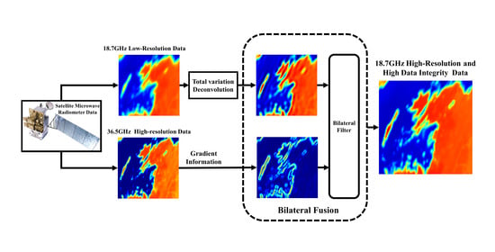
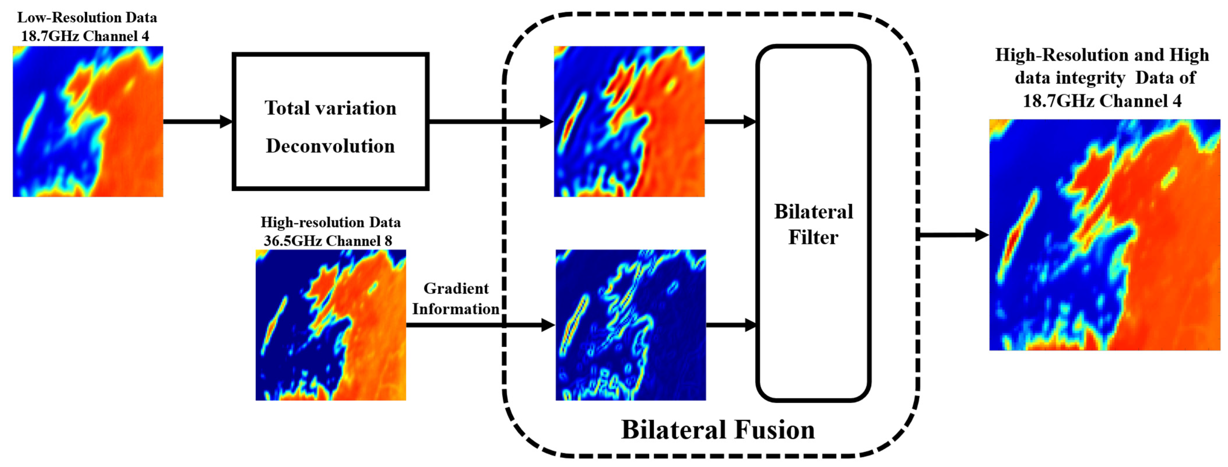
• A deconvolution algorithm based on TV regularization is proposed to reconstruct the deteriorated image aiming to enhance the spatial resolution with minimal noise amplification.
• A bilateral fusion module is cascaded with the deconvolution module to ameliorate the data integrity of reconstructed data.
• Evaluation methods are proposed to evaluate the resolution enhancement and data integrity in the coastal transition zone.

The rest of this article is organized as follows. The relevant instrument, imaging theory, and algorithm evaluation methodology are briefly described in Section 2. In Section 3, the theoretical background of the proposed method is described. Moreover, the experiment on simulated data and actual microwave radiometer imager (MWRI) measurements is performed and analyzed in Section 4. Finally, Section 5 and Section 6 draw the discussion and conclusion, respectively.

2. Related Work

2.1. MWRI Instrument

The FY-3D is the fourth generation of the Chinese FY-3 series of meteorological polar-orbiting satellites with a conical-scanning MWRI on board. It provides highly accurate measurements of the microwave emission intensity at five frequencies (10.65, 18.7, 23.8, 37, and 89 GHz) with vertical and horizontal polarization [28,29]. The spatial resolution of the MWRI image is frequency dependent, with high-frequency data having a high resolution due to the narrow beamwidth. The specific performance [29] of the FY-3D MWRI instrument is shown in

Table 1. Main characteristics of the FY3D MWRI.

Frequency (GHz)	Polarization	The Instantaneous Field of View (km)	Sampling Interval (km)	Integration Time (ms)
10.65	V/H	51 × 85	6 × 11	15.0
18.7	V/H	30 × 50	6 × 11	10.0
23.8	V/H	27 × 45	6 × 11	7.5
37	V/H	18 × 30	6 × 11	5.0
89	V/H	9 × 15	6 × 11	2.5

.

All experiments with actual measurement data are demonstrated and validated based on Level-1 (L1) data obtained by the FY-3D MWRI, which flew at an altitude of 836 km and measured the Earth’s surface brightness temperature at a 45° observation angle. The conical scanning mode is adopted, resulting in a swath of 1400 km [30]. The sampling points are $266\times 1825$ along the scan direction and the track direction. The observation footprint varies along the scanning direction due to the oblique projection of the antenna pattern. Thus, the along scan direction data is considered under the influence of relative geometry variation.

2.2. Imaging Process

The brightness temperature $T_A\left(s_0,v\right)$ obtained by the MWRI at any given frequency $v$ at the location $s=s_0$ is the convolution of the actual scene brightness temperature $T_{\mathrm{B}}\left(s,v\right)$ with the normalized antenna pattern $G\left(s_0,s,v\right)$, which can be represented by [18]

$$T_A\left(s_0,v\right)=\underset{\mathsf{\Omega }}{{\displaystyle \iint }}G\left(s_0,s,v\right)T_B\left(s,v\right)dA+n$$

(1)

where variable $s=\left(\alpha ,\beta ,\theta ,\phi \right)$ contains the longitude ($\alpha$), latitude ($\beta$), azimuth ($\theta$), and zenith angle ($\phi$). $n$ denotes the system noise.

Therefore, the actual smooth integral kernel used in Equation (1) should be the projection of the original antenna pattern on the Earth’s surface, which is calculated from the scan geometry defined by parameter $s$.

The linearity problem defined by Equation (1) can be cast in a discrete setting [25] and be expressed by:

$$m=Hf+n$$

(2)

where $f\in {ℝ}^{M\times 1}$ is a vector that denotes the unknown image $T_B$. $m\in {ℝ}^{N\times 1}$ is the vector of noise-containing measurements $T_A$. $H\in {ℝ}^{M\times N}$ is the matrix that describes a linear transformation representing the convolution operation, and $n\in {ℝ}^{N\times 1}$ is a vector corresponding to radiometric noise $NE\Delta T$.

However, in this paper, $M$ equals $N$ since the subsequent data fusion operation requires two matrices to have the same size. The general purpose of the algorithms is to recover $f$ from the degraded data $m$.

2.3. Evaluation Criteria

This paper presents several evaluation metrics to assess the reconstructed image quality from different perspectives. To objectively evaluate the overall image, the peak signal-to-noise ratio (PSNR) and structural similarity (SSIM) [31] are chosen since they are well-known for their ability to evaluate an image in terms of the similarity of the pixels in the whole image. Additionally, the noise evaluation is applied to the synthetic simulation data and it is quantitively evaluated by calculating the standard variance of the data in a flat zone.

Besides the quality of the overall image, the quality of local data in the coastal transition zones should also be considered. In particular, the capability to reconstruct spot-like targets and abrupt discontinuities related to the land–sea transition zone ought to be quantitively evaluated when noise amplification and Gibbs fluctuations are introduced. As shown in Figure 2, the simulated transect along the normal direction of the coastline demonstrates the specific situation. The absolute value of the tangent slope is defined as Resolution Factor (RF), which represents the ability to reconstruct abrupt discontinuities. The local data integrity is defined by the number of the contaminated sampling point (CP). The contaminated data has an excessive deviation from the actual $T_B$. In a complicated two-dimensional MWRI image, CP is specifically defined as the number of contaminated points in the normal direction of the local coastline.

As illustrated in Figure 2, the antenna inversion algorithm provides comparatively acceptable capabilities in terms of improving spatial resolution. Conversely, the improvement in data integrity is limited due to Gibbs fluctuations. A few sampling points are over-enhancing, which impairs data quality. Accordingly, the inversion algorithm only optimizes the data integrity for just two points in this case. However, the Gibbs fluctuations further deteriorate data integrity in some complicated scenarios. The deconvolution results are equivalent to or inferior to the original measured data.

3. Methods

The proposed algorithm is implemented according to the flowchart described in Figure 3. In this paper, 18 GHz is used as an example of low-resolution data, and 37 GHz is used as an instance of high-resolution data. The proposed algorithms can be applied in a broader frequency channel with different spatial resolutions.

Using a TV regularization deconvolution, the antenna inversion version of $T_{B-18GHz-TV}$ is obtained, which is shown in green block 1. With the intention of obtaining the noise-free and Gibbs fluctuation-free data, the Bilateral Fusion module is cascaded with $T_{B-18GHz-TV}$. The results are represented in green blocks 2 and 3, where the numbers in the green blocks represent the proposed algorithm’s restoration level. $T_{B-18GHz-TVBF}$ is obtained by Bilateral Filter operation to $T_{B-18GHz-TV}$, which aims at achieving a noise-free version. Fused with the gradient information of the 37 GHz channel to the Bilateral Filter, $T_{B-18GHz-TVBF+}$ is obtained. The Bilateral Filter and data fusion of the 37 GHz channel are combined as the proposed Bilateral Fusion module.

3.1. Total Variation Regularization Deconvolution

Since most algorithms amplify noise during image restoration, a small amount of noise in the original data may significantly impair the restoration result. To eliminate possible artifacts and noise suppression from the restoration process, specific regular terms are added to the optimization problem’s model. The TV norm is a common type of regularization [32]. The solution to the problem defined by the Equation (2) can be expressed as:

$$\underset{f}{\mathrm{minimize}}\frac{\mu }{2}\parallel Hf-m{\parallel }^2+\parallel f{\parallel }_{TV}$$

(3)

where ${\parallel ·\parallel }^2$ is the conventional L2-norm and $\mu$ is the regularization parameter,

$${\parallel f\parallel }_{TV}={\displaystyle \sum }_i\left({\left|{\Delta }_{x}f\right|}_i+{\left|{\Delta }_{y}f\right|}_i\right)$$

(4)

is the TV-norm, $i$ denotes $i$th component of $f$. ${\Delta }_x$ and ${\Delta }_y$ are the forward finite-difference operators of horizontal and vertical directions, respectively. Thus, the Equation (3) can be equivalent as follows:

$$\underset{f}{\mathrm{minimize} }\frac{\mu }{2}\parallel Hf-m{\parallel }^2+\parallel \Delta f{\parallel }_1$$

(5)

where

$$\Delta ={\left[{\Delta }_x^{\mathrm{T}} {\Delta }_y^{\mathrm{T}}\right]}^{\mathrm{T}}$$

(6)

To solve the problem defined by Equation (5), the intermediate variable $u$ can be introduced to transform the problem, which can be expressed as:

$$\underset{u}{\mathrm{minimize} }\frac{\mu }{2}\parallel Hf-m{\parallel }^2+\parallel u{\parallel }_1 \mathrm{subject} \mathrm{to} u=\Delta f$$

(7)

The augmented Lagrangian [33,34] of Equation (7) can be formulated as:

$$L\left(f,u,y\right)=\frac{\mu }{2}\parallel Hf-m{\parallel }^2+\parallel u{\parallel }_1-p^{\mathrm{T}}\left(u-\Delta f\right)+\frac{{\rho }_r}{2}\parallel u-\Delta f{\parallel }^2$$

(8)

where ${\rho }_r$ is a regularization parameter associated with the quadratic penalty term $\parallel u-\Delta f{\parallel }^2$. $p$ is the Lagrange multiplier associated with the constraint $u=\Delta f$.

The solution to Equation (8) is to find a saddle point of $L\left(f,u,y\right)$. Consequently, we use the alternating Direction Method of Multipliers (ADMM) [35] to solve the two subsequent subproblems in alternating iterations:

$$\{\begin{array}{l}\left(1\right):f_{k+1}=\underset{f}{arg min}\frac{\mu }{2}\parallel Hf-m{\parallel }^2-p_k^{\mathrm{T}}\left(u_k-\Delta f\right)+\frac{{\rho }_r}{2}{\parallel u_k-\Delta f\parallel }^2\\ \left(2\right):u_{k+1}=\underset{u}{arg min}\parallel u{\parallel }_1-p_k^{\mathrm{T}}\left(u-\Delta f_{k+1}\right)+\frac{{\rho }_r}{2}{\parallel u-\Delta f_{k+1}\parallel }^2\end{array}$$

(9)

For subproblem (1), since $L$ is derivable with respect to $f$, the solution can be obtained by taking the derivative:

$$f={ℱ}^{-1}\left[\frac{ℱ\left[\mu H^{\mathrm{T}}m+{\rho }_r{\Delta }^{\mathrm{T}}u-{\Delta }^{\mathrm{T}}p\right]}{\mu |ℱ\left[H\right]{|}^2+{\rho }_r\left({\left|ℱ\left[{\Delta }_x\right]\right|}^2+{\left|ℱ\left[{\Delta }_y\right]\right|}^2\right)}\right]$$

(10)

where $ℱ$ denotes the Fourier transform operator.

To solve the subproblem (2), a shrinkage formula [36] is introduced. Thus, the solution of $u_x$ is given as:

$$u_x=max\left\{\left|{\Delta }_{x}f+\frac{1}{{\rho }_r}{p}_x\right|-\frac{1}{{\rho }_r},0\right\}·\mathrm{sign}\left({\Delta }_{x}f+\frac{1}{{\rho }_r}{p}_x\right)$$

(11)

The solution for $u_y$ is also obtained using a similar formula as Equation (11). Therefore, the solution for the $u$-subproblem is represented as:

$$u={\left[u_x^T u_y^T\right]}^{\mathrm{T}}$$

(12)

By alternating iterations of two subproblems, the Lagrange multiplier $p$ can be updated as follows:

$$p_{k+1}=p_k-{\rho }_r\left(u_{k+1}-\Delta f_{k+1}\right)$$

(13)

The initial values $f_0=m$, $u_0=\Delta f$, $p_0=0$, and parameters ${\rho }_r=5$ are chosen. In the $k^{\mathrm{th}}$ iteration, $f_{k+1}$,$u_{k+1}$, and $p_{k+1}$ are updated sequentially according to Equations (10), (11), and (13). The convergence condition of the iterations is shown as follows:

$${\parallel f_{k+1}-f_k\parallel }_2/{\parallel f_k\parallel }_2\le {1\mathrm{e}}^{-3}$$

(14)

The result of iteration is defined as $T_{B-18GHz-TV}$, which is abbreviated as $T_{TV}.$

3.2. Data Integrity Enhancement with Bilateral Fusion

3.2.1. Bilateral Filter Denoising

However, during the process of obtaining $T_{TV}$, the spatial resolution enhancement is still achieved at the expense of noise amplification. The microwave radiometer image is steep only at the land–sea transition zone and comparatively flat in both terrestrial and marine areas. To mitigate the effects of amplified noise for the microwave radiometer image, the Bilateral Filter (BF) [37] is selected.

Bilateral Filtering is a local, nonlinear, and non-iterative technique that combines a classical Gaussian filter with an edge protection function that attenuates the filter kernel when the values between sampling points vary drastically. As brightness temperature similarities and closeness of the neighboring sampling points are considered simultaneously, the weights of the filter depend not only on geographic distance but also on the distance in brightness temperature space. The advantage of the filter is that the amplified noise in the flat regions of $T_{TV}$ is suppressed. At the same time, the coastal transition zone, which represents high-frequency information of the image, is retained. Mathematically, the Bilateral Filter output $T_{TVBF}$ derived from $T_{TV}$ is calculated as follows:

$$T_{TVBF}\left(a\right)=\frac{1}{W}{\displaystyle \sum }_{b\in S}{G}_{{\sigma }_s}\left(\parallel a-b\parallel \right)G_{{\sigma }_r}\left(\left|T_{TV}\left(a\right)-T_{TV}\left(b\right)\right|\right)\ast T_{TV}\left(b\right)$$

(15)

where $a$ is the target location, $S$ is a spatial neighborhood of $a$, $b$ is the location of adjacent sampling points in the neighborhood $S$. $\parallel ·\parallel$ denotes the geographic distance in Euclidean space, $\left|T_{TV}\left(a\right)-T_{TV}\left(b\right)\right|$ is the transition stopping function. $G_{\sigma }$ denotes the Gaussian-like kernel. ${\sigma }_r$ and ${\sigma }_s$ are the standard deviations of the Gaussian kernel.

Figure 4 depicts the effect of the Bilateral Filter, which is space-variant when applied to a real MWRI scenario. The kernel is Gaussian-like when centered inside the flat land–sea transition zone for noise reduction, while the kernel reduces to zero near the land–sea transition zone to retain the gradient variation information. In the flat zone, it is a complete Gaussian-like filter. In the land–sea transition zone, the filter is attenuated and this operation is equivalent to keeping it the same as $T_{B-18GHz-TV}$ in this area. In brief, besides cleaning the noise introduced by the TV reconstruction process mentioned above, the Bilateral Filter operation preserves the high-frequency components of the steep transition region.

3.2.2. Bilateral Fusion

The Bilateral Filter mainly suppresses the noise in the flat zone. Due to the loss of unrecoverable high-frequency information, the Gibbs fluctuations are complicated to remove. Therefore, data integrity in steep transition zones does not meet the requirements of practical meteorological applications [12].

To further eliminate noise and fluctuations, the Bilateral Fusion technique is utilized to further improve the accuracy of resolution-enhancing products. The proposed Bilateral Fusion intends to fuse the gradient information of the high-resolution image instead of the specific per-pixel values. Although the behaviors between the low- and high-frequency channels are not exactly the same, as shown in Figure 5. Their brightness temperature distribution characteristics are relatively similar in the terrestrial and marine zone, respectively. The gradient of the images is calculated with the Sobel operator. Their gradient variations are also approximate, except that the 37 GHz image has narrower gradient transition bands. In order to give a more thorough comparison of the multichannel distribution properties, the along-scan transects (labeled with the black dash-dotted line in Figure 5a) of 10.65, 18.7, 23.8, and 37 GHz brightness temperature, and the value of the land–sea mask are depicted in the Figure 5e. Their trends are analogous, with only minor fluctuations.

Specifically, the relationship between 18 and 37 GHz of the whole image can be defined as the ratio $R$:

$$R=\frac{T_{B37}}{T_{B18}}$$

(16)

As shown in Figure 6, the value of $R$ is approximately constant in the terrestrial and marine regions separately, which indicates that the brightness temperature of these two channels is roughly linear in these two areas.

Consequently, we fuse the gradient information of the 37 GHz channel measured data, which has higher resolution and no Gibbs fluctuations in the coastal transition zone, to guide the Bilateral Filtering process. The Equation (15) can be modified as follows:

$$T_{TVBF+}\left(a\right)=\frac{1}{W}{\displaystyle \sum }_{b\in S}{G}_{{\sigma }_s}\left(\parallel a-b\parallel \right)G_{{\sigma }_r}\left(\left|T_{A37}\left(a\right)-T_{A37}\left(b\right)\right|\right)\ast T_{TV}\left(b\right)$$

(17)

The simulated transect analysis explains the effectiveness of the Bilateral Fusion near the land–sea transition zone, which is shown in Figure 7. The resolution of the reconstructed image is enhanced at the expense of noise amplification in the flat zone and the Gibbs fluctuations near the steep zone.

The noise and the Gibbs fluctuations lead to the wrong land–sea zone division for the Bilateral Filter. Fused with the information of $T_{A37}$, the Bilateral Fusion properly delineates the steep and flat zone to felicitate the maximization of noise and fluctuation removal without the resolution reduction. The flat land–ocean and steep transition zones are divided according to the gradient information of 37 GHz, as illustrated by the red, green, and blue backgrounds. Notably, using the gradient information of the reconstructed deconvolution image could result in a 1~2 pixel position offset due to the Gibbs fluctuations. This mismatched region division affects the accuracy of the algorithm. In conclusion, fused with the gradient information of the high-resolution image, noise and Gibbs fluctuations are better eliminated.

4. Results

4.1. Synthetic Scenario Evaluation

In this section, synthetic simulation data and synthetic MWRI data are used to evaluate the performance of the proposed Total Variation Regularization Deconvolution and cascaded Bilateral Fusion algorithms. As a demonstration, the synthetic 18.7 GHz channel antenna temperature is generated by Equation (1), where 37 GHz channel antenna temperature is used as the scene temperature for simulation. The classic BG algorithm is used as a reference benchmark for contrast. The comparison between the results of $T_{BG}$ and our proposed $T_{TV}, T_{TVBF}, T_{TVBF+}$ are illustrated by evaluation metrics and visualization performance.

4.1.1. Synthetic Simulation Data

Quantitative analysis of resolution enhancement and data integrity assessment using actual MWRI data is challenging, and the non-uniform performance of the different frequency channels aggravates the difficulties. The synthetic simulation data depicted in Figure 8a, which has relatively regular scenes, can be alternatives. In this experiment, the synthetic scenario is characterized by a 180K background representing the ocean area. The three hot spots with gradually increased dimension and brightness temperature along the cross-scan direction indicate the small isolated islands. A large hot spot representing the continent is also generated near the small hot spots to illustrate the reconstruction performance near the abrupt discontinuities.

The degraded image is depicted in Figure 8b. The reconstruction results obtained using BG and our proposed method are depicted in Figure 8c–f. For a better visual evaluation, the local areas of the three hot spot margin of the simulated continental (enclosed by a white dash-dotted rectangle) are enlarged.

By contrasting the reconstruction results and $T_B$, all methods have sharper reconstructed fields than $T_A$. The noise in the background area of the proposed $T_{TV}$ is less than the BG method. The $T_{TVBF}$, $T_{TVBF+}$ provide noise-free images of the flat areas in visual effects. However, the Gibbs fluctuations are presented as local over-reconstruction in a two-dimensional (2D) image. The results of $T_{TVBF}$ and $T_{TVBF+}$ outperform $T_{TV}$ and BG since the Gibbs fluctuations near the transition zone are considerably mitigated.

Detailed analyses of the brightness temperature reconstruction performance are evaluated with the along-track transects (labeled with the dash-dotted line in Figure 8a), as shown in Figure 9. The ability to reconstruct the tiny target precisely is shown in area A of Figure 9. The sharpness and amplitude of $T_B$ are attenuated. All reconstruction methods improve edge sharpness to a similar degree, but the amplitude of these methods is higher than the actual value. Among them, $T_{TVBF+}$ achieves the optimum reconstruction in amplitude since it significantly alleviates the over-recovery phenomenon. The Gibbs fluctuations and the resolution factor (RF) are evaluated in area B. The RF for all methods is close. In particular, $T_{TVBF+}$ obtains a slightly better result, which is shown in

Table 2. The evaluation indices of the synthetic simulation scenario.

Methods	PSNR (dB)	SSIM	Noise	RF	CP
$T_A$	37.0367	0.9592	1.3262	15.1663	7
$T_{BG}$	38.1755	0.9642	1.8169	26.2721	7
$T_{TV}$	39.4317	0.9726	1.2427	26.1438	7
$T_{TVBF}$	40.9258	0.9936	0.0881	26.7613	3
$T_{TVBF+}$	41.0187	0.9940	0.0287	27.0301	1

. Furthermore, the $T_{TVBF}$ and $T_{TVBF+}$ demonstrate outstanding ability to reconstruct abrupt discontinuity for they overcome the Gibbs fluctuations. In area C, the noise amplification is illustrated by the degree of fluctuation. $T_{TV}$ shows a slightly better result than BG. Moreover, $T_{TVBF}$ and $T_{TVBF+}$ suppress the majority of the noise. The noise amplification is quantitively evaluated by calculating the standard variance of the data in the red dash-dotted square in Figure 8a, as shown in Table 2.

The PSNR and SSIM are evaluated over the whole image. The noise is evaluated in the flat area. The RF and CP are evaluated near the abrupt discontinuity. The experiments are performed 100 times independently for statistical evaluation, and averaged indices are shown in Table 2. Specifically, the best indices are shown in bold. The proposed $T_{TVBF+}$ outperforms other methods in terms of all five indices.

4.1.2. Synthetic MWRI Data

However, the simulated scene in Section 4.1.1 is comparatively simple since it has only horizontal and vertical components. To further test the performance of the proposed algorithm under a complicated condition, 200 images of FY3D MWRI from 1 September 2021 to 15 September 2021 are chosen. Most of these images are from the northern hemisphere. Consequently, their geographical features include sufficient gradient variation. As indicated in Figure 10, the proposed $T_{TV}$, $T_{TVBF}$, $T_{TVBF+}$ all outstrip BG in terms of PSNR and SSIM. In particular, the results of $T_{TVBF}$ are slightly better than $T_{TV}$. Furthermore, $T_{TVBF+}$ achieves the pre-eminent results.

Aiming to illustrate the reconstruction performance visually, a representative scenario around the northern region of Australia and the southern region of Indonesia is selected. The region has enough islands and a margin of mainland whose local tangent line is perpendicular to the along-track direction. As shown in Figure 11, all the algorithms produce clear boundaries and interfaces. Apparently, both $T_{TV}$ and $T_{BG}$ methods enhance the resolution at the expense of noise amplification, which can be demonstrated by the artifacts in Figure 11c,d. The results in $T_{TVBF}$ ameliorate this phenomenon and $T_{TVBF+}$ provides the outstanding performance in which almost all the artifacts introduced by noise and Gibbs fluctuations were eliminated.

For more convincing analyses of the reconstruction performance, the brightness temperature values are evaluated using the along-track transect (label with a white dash-dotted line in Figure 11a), which is shown in Figure 12. The transect is perpendicular to the local coastal line in Australia. The Australia coastal transition zone is enlarged to elaborate the ability to handle the Gibbs fluctuations.

The image sharpness of all methods’ results is approximately the same, whereas the $T_{TVBF+}$ provides the best performance with the elimination of Gibbs fluctuations. In addition, the fluctuation of $T_{TVBF+}$ in the flat zone is suppressed as well. Thus, the reconstructed $T_{TVBF+}$ produced the most satisfactory data in accordance with spatial resolution and data integrity.

A metric analysis similar to that in Section 4.1.1 is performed, which is shown in

Table 3. The averaged evaluation indices of the 200 synthetic MWRI scenarios.

Methods	PSNR (dB)	SSIM	RF	CP
$T_A$	30.2345	0.8972	26.5221	7
$T_{BG}$	35.6404	0.9048	43.8413	7
$T_{TV}$	36.5938	0.9361	43.7943	7
$T_{TVBF}$	37.3895	0.9634	43.7260	5
$T_{TVBF+}$	42.5372	0.9924	45.4776	1

. The $T_{TVBF+}$ still attains the most desirable results in PSNR, SSIM, RF, and CP. It is essential to note that the RF and CP calculation is marginally imprecise due to irregular geographic image patterns. Nonetheless, it does not affect the demonstration of the superiority of our algorithm. Therefore, these results demonstrated our methods’ effective spatial resolution and data integrity enhancement ability in practical use.

To intuitively illustrate the algorithm’s two-dimensional visual effect on complex images, another typical scene is chosen, which includes parts of the Mediterranean, continental Europe, and Africa. In addition, the image of the Peloponnese region (enclosed by the white dash-dotted rectangle) in the northern part of the Hellenic Republic and the Canakkale region (enclosed by the red dash-dotted rectangle) in the western part of Turkey is locally enlarged. In the majority of articles, the brightness temperature range of the image is set to be relatively wide [13,22], and thus the changes in detail are not readily visible visually. We adopt the strategy that sets the brightness temperature of the image to a narrow range, [250 K, 300 K], which is equivalent to adding a mask to the sea surface area. Therefore, variations in the brightness temperature of the continent can be observed more distinctly. As depicted in Figure 13, all algorithms provide a relatively sharp edge. The notable example of two enlarged regions showed the exceptional ability of $T_{TVBF+}$ to reduce artifacts and over-reconstructed details at the edge of the coastline.

In this scenario, due to the lack of coastline whose tangent line is perpendicular to the cross-track direction, the values of CP and RF are difficult to calculate. The objective evaluation indices of PSNR and SSIM are shown in

Table 4. The evaluation indices of the synthetic MWRI scenario.

Methods	PSNR (dB)	SSIM
$T_A$	29.3485	0.9045
$T_{BG}$	34.4271	0.9280
$T_{TV}$	35.7685	0.9316
$T_{TVBF}$	36.3284	0.9612
$T_{TVBF+}$	41.3148	0.9918

. The indices for $T_{TV}$, $T_{TVBF}$, and $T_{TVBF+}$ are incremental. In particular, the result obtained by $T_{TVBF+}$ is substantially ahead of other methods.

4.2. Actual MWRI Measurements Evaluation

The results shown above are based on the degenerate model. The validation of the proposed methods on actual MWRI measurements is still elusive. In this section, the actual 18.7 and 37 GHz data with the horizontal polarization are used to demonstrate the effectiveness of the proposed TV deconvolution and Bilateral Fusion. The scenarios with the same geographic area as Section 4.1.1 are selected. Since the ideal $T_B$ of 18.7 GHz is unavailable, 37 GHz data are used for reference in terms of resolution and Gibbs fluctuations in the land–sea transition zone.

As shown in Figure 14, which shows the same area as Figure 8, all the algorithms produce precise edges and interfaces for the 18.7 GHz channel. The sharpness of the enhanced resolution results is comparable to that of the 37 GHz channel. It is imperative to note that the results of both $T_{TV}$ and $T_{BG}$ introduce artifacts near the coastal transition zone of Australia, as depicted in Figure 14c,d. $T_{TVBF}$ improves this artifact to some extent and $T_{TVBF+}$ provides the best Gibbs artifact removal behavior.

Similarly, the along-track transect analysis can be applied to the actual MWRI data, as illustrated in Figure 15. There are differences in emission characteristics of 18.7 and 37 GHz channels. Nonetheless, trends in gradient changes can be used to reference since 37 GHz offers steeper variations in the abrupt discontinuities area. All methods restore the resolution of the 18.7 GHz image to a level comparable to or even exceeding that of the 37 GHz image representing a significant improvement in resolution. Furthermore, the zoomed transition zone shows $T_{TVBF+}$’s distinguished competence in eradicating the Gibbs fluctuations compared to BG and other proposed methods.

Due to the lack of the ideal label for index calculation, PSNR and SSIM are difficult to access. Moreover, RF and CP can only be approximately calculated. The indices are listed in

Table 5. The evaluation indices of the actual scenario.

Methods	RF	CP
$T_{A-37GHz}$	55.7500	3
$T_{A-18GHz}$	38.7800	5
$T_{BG}$	75.3224	7
$T_{TV}$	77.3252	7
$T_{TVBF}$	77.4811	5
$T_{TVBF+}$	78.9571	4

. Despite the increased resolution, the $T_{BG}$ method and $T_{TV}$ result in more sample points being contaminated while only $T_{TVBF+}$ improves both indices simultaneously.

Moreover, the same scene in Figure 13 is also utilized to demonstrate the capability to deal with unnatural ringing artifacts caused by over-enhancing high-frequency edges.

As shown in Figure 16, we set the color range to [240 K, 310 K] to better visually observe the terrestrial areas. $T_{TVBF}$ removes most of the artifacts introduced by $\mathrm{TV}$ deconvolution in the Canakkale region. Further, $T_{TVBF+}$ delivers nearly flawless results. For the Peloponnese region, $T_{A-18\mathrm{GHz}}$ has a noticeably blurrier edge than 37 GHz $T_A$ and only $T_{TVBF+}$ provides a pleasing enhanced-resolution product without any artifacts. Accordingly, these results demonstrated our algorithm’s superior spatial resolution enhancement and artifact suppression abilities, representing the significantly improved data integrity in practical applications.

5. Discussion

In this paper, using the proposed TVBF+ methods, the spatial resolution and the data integrity were enhanced. Experiments under one-dimensional transect analysis and visualization of two-dimensional brightness temperature demonstrate the validity and effectiveness of the proposed method. The reconstruction’s performance is further discussed quantitatively through objective metrics.

Several studies in related fields have demonstrated similar antenna inversion ability [5,17,38], but most of them do not consider the validity of the enhanced data, which are contaminated by the Gibbs fluctuations. The LW+ and Lp-penalization methods take effect to directly reduce Gibbs fluctuations during the deconvolution process [20]. In contrast, our proposed Bilateral fusion technique suppresses the Gibbs fluctuations after the deconvolution operation. High-resolution channel gradient information is used instead of pixel-level fusion [14] to avoid the problem of different behavior in a different channel. This gradient information is used as the complement of irreversible high-frequency information. The results in Section 4 demonstrated the surpassing superiority and effectiveness of the proposed method in the land–sea transition zone, which generates products with comparable resolution but relatively fewer Gibbs fluctuations and noise compared with the prevailing methods.

In addition, the 89 GHz channel has the most satisfactory spatial resolution. Theoretically, the sharpest gradient information can be extracted and exploited. However, the 89 GHz brightness temperature is susceptible to atmospheric effects, which may lead to unpredictable and unstable behavior. The tuned method of utilizing 89 GHz information needs further research. Further development will also be devoted to utilizing the ideal gradient information generated from Radiative Transfer for TOVS (RTTOV).

6. Conclusions

In this paper, to enhance the spatial resolution and data integrity, the TVBF+ method based on the TV regularization deconvolution, Bilateral Filter, and data fusion technique is proposed. The algorithm aims to improve the resolution of microwave radiometer data and simultaneously enhance data reliability. Specifically, the TV regularization deconvolution technique generates products with comparable resolution but relatively less noise than the conventional BG method. In addition, the cascaded Bilateral Filter and data fusion can ameliorate the unnatural ringing artifacts introduced by the noise and Gibbs fluctuations.

Unlike the conventional methods that mainly focus on improving the sharpness of the deteriorated image, the data integrity in the local transition zone near the abrupt discontinuities is also considered. Numerous experiments conducted in simulated and actual scenarios have substantiated the soundness of the proposed TVBF+ method, surpassing the traditional methods in accurately reconstructing measured radiometer data. The products produced with the proposed method have fewer contaminated sampling points. Thus, more microwave radiometers near the land–sea interface can be utilized for geological parameter retrieval.

References

1. Bindlish, R.; Jackson, T.J.; Wood, E.; Gao, H.; Starks, P.; Bosch, D.; Lakshmi, V. Soil moisture estimates from TRMM Microwave Imager observations over the Southern United States. Remote Sens. Environ. 2003, 85, 507–515. [Google Scholar] [CrossRef]
2. Li, X.; Zhao, K.; Wu, L.; Zheng, X.; Jiang, T. Spatiotemporal analysis of snow depth inversion based on the FengYun-3B microwave radiation imager: A case study in Heilongjiang Province, China. J. Appl. Remote Sens. 2014, 8, 084692. [Google Scholar] [CrossRef]
3. Wang, Y.; Fu, Y.; Fang, X.; Zhang, Y. Estimating ice water path in tropical cyclones with multispectral microwave data from the FY-3B satellite. IEEE Trans. Geosci. Remote Sens. 2014, 52, 5548–5557. [Google Scholar] [CrossRef]
4. Yang, H.; Zou, X.; Li, X.; You, R. Environmental data records from FengYun-3B microwave radiation imager. IEEE Trans. Geosci. Remote Sens. 2012, 50, 4986–4993. [Google Scholar] [CrossRef]
5. Sethmann, R.; Burns, B.A.; Heygster, G.C. Spatial resolution improvement of SSM/I data with image restoration techniques. IEEE Trans. Geosci. Remote Sens. 1994, 32, 1144–1151. [Google Scholar] [CrossRef]
6. Lenti, F.; Nunziata, F.; Estatico, C.; Migliaccio, M. On the spatial resolution enhancement of microwave radiometer data in Banach spaces. IEEE Trans. Geosci. Remote Sens. 2013, 52, 1834–1842. [Google Scholar] [CrossRef]
7. Long, D.G.; Brodzik, M.J.; Hardman, M.A. Enhanced-resolution SMAP brightness temperature image products. IEEE Trans. Geosci. Remote Sens. 2019, 57, 4151–4163. [Google Scholar] [CrossRef]
8. Wang, Y.; Shi, J.; Jiang, L.; Du, J.; Tian, B. The development of an algorithm to enhance and match the resolution of satellite measurements from AMSR-E. Sci. China Earth Sci. 2011, 54, 410–419. [Google Scholar] [CrossRef]
9. Chen, K.; Fan, X.; Han, W.; Xiao, H. A remapping technique of FY-3D MWRI based on a convolutional neural network for the reduction of representativeness error. IEEE Trans. Geosci. Remote Sens. 2021, 60, 1–11. [Google Scholar] [CrossRef]
10. Gentemann, C.L.; Wentz, F.J.; Brewer, M.; Hilburn, K.; Smith, D. Passive microwave remote sensing of the ocean: An overview. In Oceanography from Space; Springer: Dordrecht, The Netherlands, 2010; pp. 13–33. [Google Scholar] [CrossRef]
11. Owen, M.P.; Long, D.G. Land-contamination compensation for QuikSCAT near-coastal wind retrieval. IEEE Trans. Geosci. Remote Sens. 2009, 47, 839–850. [Google Scholar] [CrossRef]
12. Yang, J.X.; Mckague, D.S.; Ruf, C.S. Land contamination correction for passive microwave radiometer data: Demonstration of wind retrieval in the great lakes using SSM/I. J. Atmos. Ocean. Technol. 2014, 31, 2094–2113. [Google Scholar] [CrossRef] [Green Version]
13. Nunziata, F.; Alparone, M.; Camps, A.; Park, H.; Zurita, A.M.; Estatico, C.; Migliaccio, M. An enhanced resolution brightness temperature product for future conical scanning microwave radiometers. IEEE Trans. Geosci. Remote Sens. 2021, 60, 1–12. [Google Scholar] [CrossRef]
14. Maeda, T.; Tomii, N.; Seki, M.; Sekiya, K.; Taniguchi, Y.; Shibata, A. Validation of Hi-Resolution Sea Surface Temperature Algorithm Toward the Satellite-Borne Microwave Radiometer AMSR3 Mission. IEEE Geosci. Remote Sens. Lett. 2021, 19, 1–5. [Google Scholar] [CrossRef]
15. Choi, M.; Hur, Y. A microwave-optical/infrared disaggregation for improving spatial representation of soil moisture using AMSR-E and MODIS products. Remote Sens. Environ. 2012, 124, 259–269. [Google Scholar] [CrossRef]
16. Santi, E. An application of SFIM technique to enhance the spatial resolution of spaceborne microwave imaging radiometers. Int. J. Remote Sens. 2010, 31, 2419–2428. [Google Scholar] [CrossRef]
17. Backus, G.E.; Gilbert, J.F. Numerical applications of a formalism for geophysical inverse problems. Geophys. J. Int. 1967, 13, 247–276. [Google Scholar] [CrossRef] [Green Version]
18. Stogryn, A. Estimates of brightness temperatures from scanning radiometer data. IEEE Trans. Antennas Propag. 1978, 26, 720–726. [Google Scholar] [CrossRef]
19. Long, D.G.; Hardin, P.J.; Whiting, P.T. Resolution enhancement of spaceborne scatterometer data. IEEE Trans. Geosci. Remote Sens. 1993, 31, 700–715. [Google Scholar] [CrossRef] [Green Version]
20. Alparone, M.; Nunziata, F.; Estatico, C.; Lenti, F.; Migliaccio, M. An adaptive LP-Penalization method to enhance the spatial resolution of microwave radiometer measurements. IEEE Trans. Geosci. Remote Sens. 2019, 57, 6782–6791. [Google Scholar] [CrossRef]
21. Lenti, F.; Nunziata, F.; Estatico, C.; Migliaccio, M. Conjugate gradient method in Hilbert and Banach spaces to enhance the spatial resolution of radiometer data. IEEE Trans. Geosci. Remote Sens. 2015, 54, 397–406. [Google Scholar] [CrossRef]
22. Hu, W.; Li, Y.; Zhang, W.; Chen, S.; Lv, X.; Ligthart, L. Spatial resolution enhancement of satellite microwave radiometer data with deep residual convolutional neural network. Remote Sens. 2019, 11, 771. [Google Scholar] [CrossRef] [Green Version]
23. Hu, W.; Zhang, W.; Chen, S.; Lv, X.; An, D.; Ligthart, L. A deconvolution technology of microwave radiometer data using convolutional neural networks. Remote Sens. 2018, 10, 275. [Google Scholar] [CrossRef] [Green Version]
24. Li, Y.; Hu, W.; Chen, S.; Zhang, W.; Guo, R.; He, J.; Ligthart, L. Spatial resolution matching of microwave radiometer data with convolutional neural network. Remote Sens. 2019, 11, 2432. [Google Scholar] [CrossRef] [Green Version]
25. Alparone, M.; Nunziata, F.; Estatico, C.; Migliaccio, M. A multichannel data fusion method to enhance the spatial resolution of microwave radiometer measurements. IEEE Trans. Geosci. Remote Sens. 2020, 59, 2213–2221. [Google Scholar] [CrossRef]
26. Alparone, M.; Nunziata, F.; Estatico, C.; Camps, A.; Park, H.; Migliaccio, M. On the trade-off between enhancement of the spatial resolution and noise amplification in conical-scanning microwave radiometers. IEEE Trans. Geosci. Remote Sens. 2022, 60, 1–14. [Google Scholar] [CrossRef]
27. Zhou, J.; Yang, H. Noise suppression in ATMS spatial resolution enhancement using adaptive window method. In Proceedings of the 2021 IEEE International Geoscience and Remote Sensing Symposium IGARSS, Brussels, Belgium, 11–16 July 2021; pp. 7693–7695. [Google Scholar]
28. Yang, H.; Weng, F.; Lv, L.; Lu, N.; Liu, G.; Bai, M.; Qian, Q.; He, J.; Xu, H. The FengYun-3 microwave radiation imager on-orbit verification. IEEE Trans. Geosci. Remote Sens. 2011, 49, 4552–4560. [Google Scholar] [CrossRef]
29. Yang, Z.; Lu, N.; Shi, J.; Zhang, P.; Dong, C.; Yang, J. Overview of FY-3 payload and ground application system. IEEE Trans. Geosci. Remote Sens. 2012, 50, 4846–4853. [Google Scholar] [CrossRef]
30. Tang, F.; Zou, X.; Yang, H.; Weng, F. Estimation and correction of geolocation errors in FengYun-3C microwave radiation imager data. IEEE Trans. Geosci. Remote Sens. 2015, 54, 407–420. [Google Scholar] [CrossRef]
31. Wang, Z.; Bovik, A.C.; Sheikh, H.R.; Simoncelli, E.P. Image quality assessment: From error visibility to structural similarity. IEEE Trans. Image Process. 2004, 13, 600–612. [Google Scholar] [CrossRef] [Green Version]
32. Chan, T.F.; Wong, C.-K. Total variation blind deconvolution. IEEE Trans. Image Process. 1998, 7, 370–375. [Google Scholar] [CrossRef] [Green Version]
33. Rockafellar, R.T. Augmented Lagrangians and applications of the proximal point algorithm in convex programming. Math. Oper. Res. 1976, 1, 97–116. [Google Scholar] [CrossRef]
34. Chan, S.H.; Khoshabeh, R.; Gibson, K.B.; Gill, P.E.; Nguyen, T.Q. An augmented Lagrangian method for total variation video restoration. IEEE Trans. Image Process. 2011, 20, 3097–3111. [Google Scholar] [CrossRef] [PubMed]
35. Gabay, D.; Mercier, B. A dual algorithm for the solution of nonlinear variational problems via finite element approximation. Comput. Math. Appl. 1976, 2, 17–40. [Google Scholar] [CrossRef] [Green Version]
36. Li, C. An Efficient Algorithm for Total Variation Regularization with Applications to the Single Pixel Camera and Compressive Sensing; Rice University: Houston, TX, USA, 2010. [Google Scholar]
37. Tomasi, C.; Manduchi, R. Bilateral filtering for gray and color images. In Proceedings of the Sixth International Conference on Computer Vision (IEEE Cat. No. 98CH36271), Bombay, India, 4–7 January 1998; pp. 839–846. [Google Scholar]
38. Long, D.G.; Daum, D.L. Spatial resolution enhancement of SSM/I data. IEEE Trans. Geosci. Remote Sens. 1998, 36, 407–417. [Google Scholar] [CrossRef] [Green Version]
Figure 1. Illustration of the proposed spatial resolution and data integrity TVBF+ method.
Remotesensing 14 03502 g001
Figure 2. Pictorial view of the Resolution Factor and contamination area with the normal transect near the abrupt discontinuity.
Remotesensing 14 03502 g002
Figure 3. The flowchart of the proposed method. (The blue blocks denote the observations collected by MWRI. The green blocks denote the output of the proposed methods and the number in the upper right corner of the green blocks denotes the level of the restoration).
Remotesensing 14 03502 g003
Figure 4. Illustration of the Bilateral Filter’s denoising operation in an actual MWRI scenario. (In the center of the figure is the performance of the spatial-variant Bilateral Filter at different geolocation positions).
Remotesensing 14 03502 g004
Figure 5. Performances of the different frequency channels. (a) 18.7 GHz Vertical Polarization scene temperature; (b) 37 GHz Vertical Polarization scene temperature; (c) the gradient of 18.7 GHz Vertical Polarization scene temperature; (d) the gradient of 37 GHz Vertical Polarization scene temperature; (e) the along-track transects of the synthetic scenario (labeled with the dash-dotted line in (a)).
Remotesensing 14 03502 g005
Figure 6. Value of R in actual MWRI scene with horizontal and vertical polarization. (a) Value of R for Vertical Polarization; (b) value of R for Horizontal Polarization.
Remotesensing 14 03502 g006
Figure 7. Simulated performance of 18 and 37 GHz near the transition zone with abrupt discontinuity.
Remotesensing 14 03502 g007
Figure 8. The synthetic scenario and resolution enhancement results. (a) Synthetic 18.7 GHz scene temperature; (b) simulated 18.7 GHz antenna temperature; (c) the Backus–Gilbert enhancement results; (d) the TV enhancement results; (e) the TVBF enhancement results; (f) the TVBF+ enhancement results.
Remotesensing 14 03502 g008
Figure 9. The along-track transects of the synthetic scenario (labeled with the dash-dotted line in Figure 8).
Remotesensing 14 03502 g009
Figure 10. The evaluation indices of the 200 images. (a) PSNR; (b) SSIM.
Remotesensing 14 03502 g010
Figure 11. The synthetic MWRI scenario and resolution enhancement results. (a) Synthetic 18.7 GHz scene temperature; (b) simulated 18.7 GHz antenna temperature; (c) the Backus–Gilbert enhancement results; (d) the TV enhancement results; (e) the TVBF enhancement results; (f) the TVBF+ enhancement results.
Remotesensing 14 03502 g011
Figure 12. The along-track transects of the synthetic MWRI scenario (labeled with the dash-dotted line in Figure 11a).
Remotesensing 14 03502 g012
Figure 13. The synthetic MWRI scenario and resolution enhancement results. (a) Synthetic 18.7 GHz scene temperature; (b) simulated 18.7 GHz antenna temperature; (c) the Backus–Gilbert enhancement results; (d) the TV enhancement results; (e) the TVBF enhancement results; (f) the TVBF+ enhancement results. (The image in the bottom-left corner is a partial enlargement of the white dotted square and the image in the bottom-right corner is a partial enlargement of the red dotted square).
Remotesensing 14 03502 g013
Figure 14. The actual MWRI scenario and resolution enhancement results. (a) Actual 37 GHz scene temperature; (b) actual 18.7 GHz antenna temperature; (c) the Backus–Gilbert enhancement results; (d) the TV enhancement results; (e) the TVBF enhancement results; (f) the TVBF+ enhancement results.
Remotesensing 14 03502 g014
Figure 15. The along-track transects of the actual scenario (labeled with the dash-dotted line in Figure 14).
Remotesensing 14 03502 g015
Figure 16. The actual MWRI scenario and resolution enhancement results. (a) Actual 37 GHz scene temperature; (b) actual 18.7 GHz antenna temperature; (c) the Backus–Gilbert enhancement results; (d) the TV enhancement results; (e) the TVBF enhancement results; (f) the TVBF+ enhancement results. (The image in the bottom-left corner is a partial enlargement of the white dotted square and the image in the bottom-right corner is a partial enlargement of the red dotted square).
Remotesensing 14 03502 g016