
RSEDM: A New Rotational-Scan Exponential Decay Model for Extracting the Surface Urban Heat Island Footprint


1
School of Geographical Sciences, Nantong University, Nantong 226007, China
2
Department of Land Surveying and Geo-Informatics, The Hong Kong Polytechnic University, Hong Kong 999077, China
*
Author to whom correspondence should be addressed.
Remote Sens. 2022, 14(14), 3505; https://doi.org/10.3390/rs14143505
Submission received: 21 June 2022
/
Revised: 19 July 2022
/
Accepted: 20 July 2022
/
Published: 21 July 2022
(This article belongs to the Section Urban Remote Sensing)
Abstract
:Surface urban heat islands are widely focused on due to their close relationship with a series of environmental issues. Obtaining a precise footprint is an important prerequisite for heat island research. However, the land surface temperature curves used for calculating footprint are affected by factors such as the complexity of land-use types, thereby affecting the accuracy of footprint. Therefore, the rotational-scan exponential decay model is developed in this paper, which first takes the gravity center of an urban area as the origin of polar coordinates, specifies due north as the starting direction, and rotationally scans the suburbs that are within 20 km outside urban areas in a clockwise direction at an angle of 1°. The eligible suburbs are screened out according to the built-up area rate, water body rate, and merge tolerance. Then, exponential decay fitting of the temperature curve is performed to obtain the extension distance of the heat island and the background temperature, which are used to determine the final footprint. Based on the method, the footprints of 15 cities were calculated and compared with those of the traditional method. The results show that: (1) this method could effectively eliminate the influence of a large number of contiguous built-up areas and water bodies in the suburbs on the footprint calculation, thus greatly improving the accuracy of the temperature curve and footprint. (2) Three of four cities had the largest footprint boundary in spring. All four cities had the strongest heat island intensity in summer and the smallest footprint boundary and intensity in winter. (3) Coupling effect would aggravate the negative impact of heat islands in the suburbs and threaten the suburban environment. As a state-of-the-art method, it can enhance the calculation accuracy and precisely reflect the spatial pattern of footprint, which is of great significance for the sustainable development of cities.
1. Introduction
Many cities around the world have experienced rapid expansion [1]. Currently, more than half of the world’s population now lives in urban areas, and the proportion is expected to reach 67% by 2050 [2]. The increasing intensity of human activity and the centralization of energy consumption have significantly altered the land surface characteristics and the energy balance of the cities [3,4], leading to various environmental issues. Among these issues, the urban heat island (UHI), defined as the phenomenon of the urban area being warmer than its surrounding suburban area [5,6], is a key subject. The UHI effect exacerbates the negative impacts on urban areas, such as energy consumption [7,8] and urban ecological damage [9,10]. Moreover, it poses a great threat to the health of residents [11,12,13], thus, it has received considerable widespread attention [14,15,16].
There are two types of UHI, namely atmospheric UHI (AUHI) and surface UHI (SUHI) [17]. The AUHI is quantified using air temperature records based on ground meteorological stations or site measurements [18,19], while the lack of continuous ground stations makes it unable to express the spatial pattern of the UHI effect well. With the development of remote sensing technology, sufficient land surface temperature (LST) data have been provided, with wide coverage and periodic observation, filling the gaps in AUHI and promoting studies of SUHI. Currently, studies on SUHI are generally divided into three categories: spatiotemporal variation, driving mechanism, and environmental impact. The first category focuses on exploring the spatial patterns and temporal variations of SUHI [20,21,22]. The second category examines the driving forces of SUHI [23,24]. The third category illustrates the impact of SUHI on the urban environment and provides targeted mitigation policies [25,26].
SUHI intensity (SUHII) and SUHI footprint (FP) are the two main indicators that can quantify SUHI. SUHII, which is described as the temperature difference between urban areas and suburban areas [27,28,29], is one of the most commonly used indicators. The relationship between SUHI spatial patterns and land-use cover is systematically elaborated via SUHII [29,30]. However, SUHII is unable to comprehensively quantify the SUHI effect, as it focuses more on the temperature values while ignoring the spatial extent of the SUHI effect. The range of the SUHI effect can reach several times the urban area [31], so it is necessary to understand the spatial patterns of the SUHI effect.
Subsequently, the SUHI FP, defined as the extent of the increased LST with regard to the suburban region, can be introduced as a new indicator to delineate the spatial morphology of the SUHI effect [32]. The advantage of the SUHI FP is that it can take both the magnitude and the spatial extent of the SUHI effect into account. Several algorithms have been developed to calculate the SUHI FP. The Gaussian surface method is widely used to characterize the SUHI FP due to its excellent modeling performance [33,34,35]. However, this method pays more attention to describing the trajectory of the SUHI gravity center. The FP delineated by this method is an ellipse, which does not accurately represent the true spatial extent of the SUHI effect. To obtain the accurate FP, the exponential decay model (EDM), which delineates the FP by calculating the extension distance of the SUHI effect through fitting LST curves, is proposed. Previous studies focused on a single city and revealed the relationship between FP and urban size [36]. Later, the study area was extended to urban agglomerations, and the impact of the spatial structure of urban agglomerations on the SUHI FP was emphasized [37]. However, the EDM does not eliminate the uncertainties associated with land-use type and the influence of the SUHI coupling effect between neighboring cities, which could decrease the accuracy of the LST curves. The LST curve in this method is crucial because it determines the final FP, but few studies have explored the accuracy of the curve.
In terms of the study region, the SUHI first arises in large and medium-sized cities in developed countries due to the early start of the urbanization process. With the rapid economic development of some developing countries, cities with populations of more than 1 million or even 10 million have also emerged and begun to replicate the heat environment problems faced by cities in developed countries [38,39]. However, from the perspective of SUHI evaluation, the generation mechanisms and evaluation methods of both are basically the same, and the research results of SUHI have strong universal applicability [40]. Existing studies have pointed out that water bodies and terrain can decrease the LST, thereby affecting the quantification of the SUHI effect [41,42,43]. Therefore, most of the FP calculations remove the water bodies and terrain. On the other hand, some studies state that built-up areas can increase LST [44,45], but the influence of built-up areas outside the urban area is less often taken into account when using traditional methods such as the EDM, which decreases the extraction accuracy of the FP. The complexity and irregularity of urban expansion lead to uneven distribution of landscapes around the urban area, which increases the uncertainty of the LST curve, resulting in the over and underestimation of the FP [46].
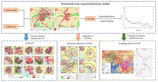
Given the above analysis, this study aims to develop an optimization method called the rotational-scan exponential decay model (RSEDM) for SUHI FP calculation. The innovation is to fully consider the influence of water bodies and unevenly distributed built-up areas outside urban areas on the FP and to use rotational scan to exclude these areas and improve the accuracy of the LST fitting curve, thus obtaining a more accurate FP.
The research objectives of this study are as follows: (1) to improve the accuracy of LST curves so as to obtain an accurate FP by developing RSEDM; (2) to clarify the characteristics of the SUHI FP by using RSEDM and the advantages of RSEDM compared with traditional methods; (3) to apply the RSEDM to the exploration of the seasonal variations of SUHI effect; (4) to reveal the SUHI coupling effect between neighboring cities. Therefore, the remainder of this paper is organized as follows: Section 2 introduces the relevant data and processing flow. The SUHI FP results are illustrated in Section 3. Section 4 and Section 5 provide the discussion and conclusion, respectively.
2. Materials and Methods
To remove the influence of water bodies and built-up areas around urban areas, this paper proposes RSEDM to calculate the SUHI FP accurately. This methodology includes three steps: (1) data processing: extracting the urban areas from nightlight (NTL) images and deriving the LST from Landsat images on the Google Earth Engine (GEE) platform; (2) SUHI FP calculation: screening the suburbs less affected by built-up areas and water bodies by rotational scan, and fitting the suburban LST curve to calculate FP; (3) analysis: carrying out a series of analyses of the results (Figure 1).
2.1. Study Area
The Yangtze River Delta urban agglomeration (YRDUA) is located along the central eastern coastline of China. It is one of the most densely populated and economically developed areas in China. In the past few decades, the YRDUA has experienced rapid urbanization, which has brought serious thermal environmental problems [47]. Several essential characteristics were used to decide the study area based on the China Statistical Yearbook of 2020, including (a) large population (over 4.5 million permanent residents), (b) high GDP (over CNY 500 billion), (c) frequent heatwaves over the decade, and (d) Landsat 8 data availability. Thus, the target area included 15 cities in the YRDUA, namely, Changzhou (CZ), Hangzhou (HZ), Hefei (HF), Jiaxing (JX), Nanjing (NJ), Nantong (NT), Ningbo (NB), Shanghai (SH), Shaoxing (SX), Suzhou (SZ), Taizhou (TZ, Jiangsu Province), Taizhou (TZ, Zhejiang Province), Wuxi (WX), Yancheng (YC), and Yangzhou (YZ), as shown in Figure 2. The total area is about 130,000 km2, and the terrain is flat.
2.2. Data
The data used in this study included Landsat 8 images, NTL images, land-use data, and built-up area statistical data for 2020.
2.2.1. Remote Sensing Images and Processing
All of the Landsat 8 data for the four seasons in 2020 were provided by the United States Geological Survey (USGS). Landsat 8 data with red, near-infrared (NIR) had a 30 m spatial resolution. The data from the Landsat series were considered to be consistent and intercalibrated, so thermal infrared (TIR) bands were also resampled to 30 m spatial resolution. The LST data were retrieved on the GEE platform by accessing the code (accessed on 15 March 2022).
The VIIRS NTL, collected by the NASA–NOAA Suomi National Polar-Orbiting Partnership Satellite, had the unique ability to record emitted visible and near-infrared (VNIR) radiation at night, with a spatial resolution of 500 m. NTL data for 2020 were clipped and downloaded on the GEE platform to extract urban areas (accessed on 20 March 2022).
2.2.2. Land-Use Data and Statistical Data
Land-use data for 2020 were acquired from the Resource and Environmental Science Data Center of the Chinese Academy of Science [48], with a spatial resolution of 100 m (accessed on 22 March 2022). These data were generated based on Landsat TM remote sensing image interpretation, including six primary classes, namely, farmland, forest, grassland, water, build-up area, and unused land. In addition, the built-up area data were obtained from the China Statistical Yearbook [49] (accessed on 22 March 2022). Land-use data and area statistical data were used to analyze the impact of land use on FP calculation and to correct the urban area extracted from the NTL images, respectively.
2.3. Approaches
2.3.1. LST Retrieval
The statistical mono-window (SMW) algorithm was used to retrieve LST with the GEE platform [50,51,52]. The approach was based on the empirical relationship between top-of-atmosphere (TOA) brightness temperatures and LST; the formula was as follows:
where represents the TOA brightness temperature in the TIR channel, while represents the surface emissivity for the same channel. The algorithm coefficients , , and are determined by linear regressions of radiative transfer simulations performed for 10 classes of total column water vapor (TCWV) (i = 1, …, 10).
2.3.2. Urban Area Extraction
The urban area was extracted from NTL images based on the dichotomy method [53]:
where is the segmented binary image, is the threshold, and is the pixel value of the original image at row and column . To obtain an accurate urban area, the threshold was continually adjusted until the area was closest to the reference data. Only the main built-up area with the largest area was considered an urban area.
2.3.3. SUHI FP Calculation
The SUHI effect decays exponentially with distance from the urban areas to the suburbs [36]. Built-up areas and water bodies distributed around the urban areas affect the LST, the former increases the LST [54], while the latter offsets the impact of urbanization on the LST in the suburbs [42], causing deviation in the fitting of the LST curves. In order to eliminate these deviations to obtain a suitable LST curve for the suburban area, this study proposed the rotational-scan exponential decay model (RSEDM) to calculate FP. The RSEDM consists of the following three steps:
(1) Taking the gravity center of the urban area as the origin of polar coordinates, the suburbs 20 km outside the urban area was scanned clockwise with an angle of 1° starting from the north. If the proportion of built-up area exceeded the BR or the proportion of water body exceeded the WR within a sector of 1°, then the sector was excluded. After scanning, part of the excluded area was merged with the neighboring reserved area according to the MT. The final selected suburban area was less impacted by built-up areas and water bodies. The BR, WR, and MT were three vital parameters in this method. The BR and WR were the built-up area rate and water body rate, representing the threshold of the proportion of built-up area and water body in a 1° sector, respectively; they were used to judge whether to reserve the area. MT was the merge tolerance. When the excluded area was too small, the LST curve was not actually affected, so if the continuous excluded area was smaller than MT, it would be merged into the reserved area next to it. These three parameters can be changed according to the actual situation.
(2) To obtain the LST curves, multiple ring buffers were drawn from the urban area boundary to the selected suburbs at 1 km intervals. The mean LST of each ring was calculated and drawn to a curve. The exponential decay function was utilized to quantitatively analyze the changes in LST (Figure 3). The formula is as follows:
where is the mean LST of each ring, is the SUHII, is the exponential decay rate, is the extension distance of the FP, which is the distance from the boundary of the urban area to the buffer ring, and represents the fitted background LST, namely, the LST in the suburban area that is not affected by the SUHI effect.
(3) The final SUHI FP was determined by and . Specifically, a rough FP boundary was first delineated according to , and then the pixels within the boundary that was higher than were further extracted. The extracted FP result eliminated the influence of large water bodies and green spaces.
3. Results
3.1. The Characteristics of SUHI FP
In this study, the BR and WR were set to 30%, and MT was set to 5°, according to the experimental experience. The extension distance d and the rural background T0 of the SUHI effect in 15 cities were calculated using the RSEDM (Table 1). The d values ranged from 3.78 km to 15.97 km. SX had the smallest d, while YC had the largest. More than half of the cities had a d value greater than 10 km, indicating that the influence range of the SUHI effect was relatively wide in the YRDUA. T0 ranged from 29.84 °C to 40.05 °C, and most cities had T0 smaller than 35 °C, but there were still a few suburbs that suffered from the threat of high LST.
According to the d and T0, the final SUHI FPs of 15 cities were delineated (Figure 4). Through scanning, suburban areas affected by large and continuous built-up areas and water bodies were effectively excluded from the area that was used for LST curve fitting. The spatial morphology of the FP was not a simple urban expansion form but an irregular range without the abnormally low LST area, reflecting strong anisotropy.
The results showed that SH had the largest SUHI FP of the 15 cities, with an area of 4466.73 km2, while TZ (ZJ) had the smallest FP, with an area of 291.28 km2. SH, as the city with the largest FP area, did not have the largest SUHI extension distance, while TZ, as the city with the smallest FP area, also did not have the smallest extension distance. There was no direct link between SUHI extension distance and FP area. Thus, we further considered the relationship between urban size and FP area. The results showed that the FP reached a maximum of 6.7 times the urban area. Meanwhile, there was a positive linear relationship between the FP area and urban size (r = 0.88, p < 0.05) (Figure 5). Therefore, the FP area increased depending not on the extension distance of SUHI effect but on the size of the built-up area.
3.2. Comparative Analysis between the RSEDM and EDM
3.2.1. Spatial Differences in FP Calculated by the RSEDM and EDM
To validate the effectiveness of the proposed RSEDM, we compared the SUHI FPs of 15 cities calculated by the EDM and RSEDM, respectively. The area difference between the two methods ranged between 19.69 km2 and 1303.49 km2 (Table 2). Cities with large area differences were divided into two types. The first type was that the FP area calculated by RSEDM was larger than that of EDM, such as NT. Since the southwestern area of the city was the Yangtze River, this big water body caused great interference to the fitting results of the LST curve, which made the FP extension distance calculated by EDM too small (Figure 6a). Although the calculated FP of EDM included areas not affected by the SUHI effect, such as large water bodies and other cities across the Yangtze River, its area was still smaller than the FP calculated by RSEDM. The second was that the FP area of RSEDM was significantly smaller than that of EDM, such as NB (Figure 6b). The city not only had a large area of water in the northeast but also built-up areas surrounded by a large area of forest land. These features had a cooling effect on the urban LST and were not affected by the SUHI. However, the EDM mistook these low LST regions as FP in these types of cities. In conclusion, the FP boundaries obtained by RSEDM terminated in low LST areas such as water bodies and green spaces, unlike EDM, which simply extended the built-up area boundaries outward. The FP obtained by RSEDM was anisotropic in shape, it can better reflect the spatial differences of SUHI patterns, which was obviously more scientific and reasonable.
3.2.2. Advantages of the RSEDM in Fitting Background LST
To further understand the differences in principle between the RSEDM and EDM, we divided 15 cities into two categories based on land-use type outside urban areas and compared the SUHI FP of these two types of cities calculated by the two methods. Specifically, this study first classified cities according to the overall proportion of built-up area and water body in suburban areas within 20 km of 15 cities. The overall proportion of built-up area and water body in the first category was less than 20%, including HF, NB, SX, TZ (JS), and YC. The second category cities with a proportion greater than 20% included 10 cities, namely, CZ, HZ, JX, NJ, NT, SH, SZ, TZ (ZJ), WX, and YZ.
T0 is the LST of a suburban area that is not affected by the SUHI effect. This study compared the fitted background LST with the real background LST to judge the accuracy of the RSEDM. The average LST of the three farthest buffer rings was used as the real background LST for each city since the distances of these buffers were obviously larger than the previously reported FP [55].
For the first category of cities, the RSEDM can obtain accurate background LST. Table 3 shows the background LST fitted by the two methods and the difference between them and the real background LST. When using RSEDM, the fitted background LST was higher than the real background LST for two cities and lower for three cities. When using the EDM, the fitted background LST of three cities was higher than the real background LST, while two cities were lower than that. The difference between the background LST calculated by the two methods was not significant, ranging only from 0.06 °C to 0.5 °C. In general, most of the cities in the first category obtained background LST that were closer to the true value used for RSEDM compared to EDM.
In the second category of cities, the RSEDM had a better performance than the EDM (Table 4). The background LST fitted by the RSEDM in 7 of the 10 cities was closer to the real background LST. Compared to the EDM, the RSEDM could improve the accuracy of the background LST in the range of 0.18 °C to 1.28 °C. The remaining three cities, CZ, SZ, and WX, seemed not to work well when using the RSEDM. The fitted background LST of these three cities was quite different from the real background LST, and all were less than the real LST. The difference between the fitted LST and the real LST in CZ, SZ, and WX was 0.88 °C, 0.84 °C, and 0.73 °C, respectively. Considering that the cities in the Su-Xi-Chang region are well established and are almost connected in space, the real background LST of these three cities may be higher than it should be, resulting in the background LST fitted by the RSEDM not being close to the real LST. However, it did not mean that the RSEDM was unsuitable for these cities.
The background LST is the suburban LST at the periphery of the FP boundary, so its accuracy reflects the accuracy of the whole FP. In general, the RSEDM performed better in obtaining the background LST to calculate the SUHI FP accurately, especially for the second category of cities.
3.2.3. Advantages of the RSEDM in R2
The SUHI effect decays exponentially with the distance away from the urban area. The LST curve showed that there was a large LST difference between the urban area and the suburbs at first, and then the LST gradually decreased until the suburban area, where the curve flattened out because the suburban area was not affected by the SUHI effect. When fitting with an exponential decay function, the higher the R2, the more accurate the fitting result. However, it was found that the R2 of some cities was not high when using the EDM, which indicated that the LST curves of these cities were not exactly exponentially decaying due to the land-use type. The LST curve obtained by the EDM contained many uncertain factors, the most intuitive of which was the influence of built-up areas outside the urban areas, and the RSEDM was designed to remove these uncertainties.
Taking NJ as an example (Figure 7), the R2 was only 0.67 when using the EDM. This was because the EDM took the largest built-up area of the city as the urban area, while the built-up area of NJ was divided into two parts by the Yangtze River, so the LST curve was influenced by the other built-up areas, causing the LST to increase from 34.18 °C in the fourth ring to 34.69 °C in the sixth ring. The EDM was unable to directly address the abnormal rise in the LST curves, resulting in low fitting accuracy. Thus, if the selected urban area is surrounded by too many other built-up areas, it will lead to the SUHI coupling effect and the “pseudo cold island” phenomenon, which will bias the SUHI FP calculation.
The advantage of the RSEDM is that the abnormal LST areas in a certain direction were excluded, making the LST variation more consistent with exponential decay and, thus, improving the curve fitting accuracy. For the first category of cities, the RSEDM performed a good fitting function, and the R2 values were all greater than 0.8. For the second category of cities, the R2 values ranged from 0.77 to 0.97. In 9 of the 10 cities, the R2 obtained by the RSEDM was greater than that obtained by the EDM, with the increment ranging from 0.01 to 0.5 (Figure 8). The R2 increased most significantly in four cities, JX, NJ, SZ, and TZ (ZJ). When the exponential fit was performed using EDM, the LST curves had obvious up and down fluctuations with the increase of ring buffers, where the smallest R2 was only 0.41. After being corrected by RSEDM, the anomalously high LST in four cities were reduced, the pattern of the LST change was more consistent with exponential decay, and the fitted curves were closer to the real ones. Meanwhile, the curve fitting accuracy in the remaining cities was also improved to some extent. Therefore, in terms of fitting R2, the RSEDM was better than the EDM at excluding the impact of built-up area to calculate a more accurate SUHI FP.
3.3. Seasonal Variations of SUHI
In this study, we applied RSEDM to the exploration of the seasonal variations of SUHI. Specifically, we selected HF and YC from the first category of cities and NJ and NT from the second category of cities. Taking these four typical cities as examples, we calculated their SUHI FP and SUHII in four seasons of 2020, respectively.
3.3.1. Spatiotemporal Variations of SUHI FP
Spatially, HF had the largest FP in summer, while the other three cities all had the largest FP in spring, meaning that more suburban areas would be negatively affected by the SUHI effect in spring. In winter, the FP of all cities were the smallest, the SUHI effect had less impact on surrounding suburbs than in other seasons. From spring to winter, the FP of HF increased first and then decreased while the FP of NT continued to diminish. The FP of YC and NJ decreased from spring to summer, increased from summer to autumn, and finally decreased from autumn to winter (Figure 9).
The mean center was used to identify the geographical center of the SUHI effect. From spring to winter, the mean center of FP of HF generally moved to the southeast, and there was a crossover in its track. The mean center of YC had a round trip between spring, summer, and autumn, eventually moving northwest. For NJ, the track formed a closed loop, with the mean center in spring being very close to that in winter. Moreover, the track of NT was more straightforward, generally moving southwest.
3.3.2. Temporal Variations of SUHII
The SUHII is the temperature difference between the urban and the suburban area. The larger the difference, the more severe the SUHI effect. The maximum values of SUHII in four cities all occurred in summer, with the highest intensity reaching 5.50 °C. Similarly, the minimum values were all in winter, with a minimum of 0.55 °C (Figure 10a). SUHII of all four cities showed an upward trend from spring to summer and a downward trend from summer to winter. The maximum values of spring, summer, and autumn appeared in YC, and that of winter was in NJ. From the perspective of seasonal changes, only the trend of SUHII in HF corresponded to the trend of the FP area, while the other three cities did not meet this characteristic. From Figure 10b, it can be seen that the largest FP in spring was NJ, with an area of 1852.44 km2. While in other seasons, HF had the largest FP, especially in summer, with an area of 2526.05 km2 which was much larger than other cities. The FP area in HF increased from spring to summer and decreased from summer to winter. The FP of YC and NJ showed a decreasing trend from spring to summer, then rebounded from summer to autumn, and finally decreased to a minimum in winter. Additionally, NT decreased from spring to winter continually. All four cities had the smallest FP areas in winter, indicating that the SUHI effect was weakest in winter. Therefore, high SUHII did not imply that the SUHI effect could affect a broader area.
4. Discussion
4.1. Effect of Parameter Threshold
Parameter settings lead to different extraction results for the SUHI FP. To reveal how the BR, WR, and MT affected the extraction results, experiments were conducted in the city of NJ.
The influence mechanisms of BR and WR on FP were similar, but the effect was the opposite. The larger the BR, the more built-up areas were included, leading to an increase in LST and making the LST curve appear abnormally high. Conversely, the increase in the WR significantly reduced the mean value of the LST. Therefore, this study set a series of different parameter values to analyze the influence in detail. Here, only 10%, 30%, and 50% were selected as the values of BR and WR for purposes of illustration. The selected suburban area and FP are shown in Figure 11. When the BR and WR were 10%, the fitted background LST was 1.2 °C lower than the actual value, and the FP area was the largest at 3644.52 km2. However, the R2 was only 0.22, and it was difficult to guarantee the accuracy of the FP at this time. When the threshold was set too low, only a few suburban areas were preserved, so the attenuation effect of SUHI was not really reflected. When the BR and WR were 50%, R2 was 0.67, and the FP area was the smallest, at 1181.31 km2. The LST curve still had a significant upward trend in the 4th ring and the 12th ring, indicating that when the threshold was set too high, the influence of land-use type could not be well eliminated. If the threshold was set to 30%, R2 was the highest, reaching 0.86, and the difference between the fitted and the real background LST was the smallest, at only 0.07 °C, indicating that the FP was the most reasonable.
The MT value could also cause inaccuracy of the FP. This parameter determined the area of the exclusion region. When the MT was too large, a large number of culled areas were merged into the suburbs used to calculate the LST curve, while excessively fine patches were excluded, and these areas would not actually affect the LST curve. Therefore, after setting the BR and WR thresholds at 30%, this study took 5°, 10°, and 20° as examples to analyze the influence of the MT on the SUHI FP. The selected suburb areas and FP results are shown in Figure 11. With the increase in the MT, R2 gradually decreased, and the difference between the fitted and the actual background LST became larger. When the tolerance was 5°, the abnormal increase in LST could be slowed down to the greatest extent, and the LST curve fitting was the best.
In general, if the thresholds of the BR, WR, and MT were set too small, the selected suburbs would be small and scattered. On the other hand, most of the suburbs were reserved, making it impossible to completely exclude the impact of built-up areas and water bodies. This ultimately led to the FP being overestimated or underestimated. For the cities in this study, 30% and 5° were the most appropriate thresholds, but the optimal threshold was not set in stone. For cities in other regions, the optimal threshold should be selected according to their own characteristics.
4.2. SUHI Coupling Effect in the Su-Xi-Chang Metropolitan Area
Three cities in the Su-Xi-Chang metropolitan area are geographically close, and all have experienced very rapid urban expansion, so the coupling effect of SUHI can be observed in the adjacent cities. Wuxi city, located in the center of the metropolitan area, was used as an example to study the SUHI coupling effect. LST curves were drawn separately according to the selected sectors, with a BR value exceeding 30% between Wuxi and Changzhou and between Wuxi and Suzhou, as shown in Figure 12. The SUHI effect in the direction of Changzhou decreased at first, but unlike the normal trend, it increased gradually from the 11th ring. This was because suburbs between the two cities were affected by the coupling effect, which intensified the negative effects of the SUHI.
The SUHI effect in the direction of Suzhou had an upward trend, reaching a maximum of 39.32 °C in the 14th ring, which was much higher than the temperature at both ends, while the LST gradually decreased after the 14th ring. This indicates that Suzhou had a more serious impact on Wuxi than Changzhou. On the whole, the LST in the suburbs of Wuxi had a serious abnormal rise under the combined action of the two cities. Therefore, the coupling effect of the SUHI poses a great threat to the suburban environment.
4.3. Difference between Popular Methods
The RSEDM contributed to a comprehensive understanding of the SUHI effect. It provided accurate FP in space as well as SUHII in quantity. Based on the idea of anisotropy, the current SUHI FP study can be divided into two categories. Firstly, the FP calculated by EDM was simply a rough range (Figure 13a). The result was derived based on the isotropy, so it only presented the expansion form of the urban areas and inevitably includes some low LST areas. Moreover, it only excluded the impact of water bodies but ignored the built-up areas surrounding the urban areas [36]. The detailed comparative analysis was described in Section 3.2. Secondly, some studies had realized the anisotropy of the SUHI effect. The Gaussian surface method had been used in SUHI modeling to reflect the directionality of the urban heat distribution [56,57]. However, it can only represent the difference of the SUHI effect in the direction of the long and short axes of the ellipse and cannot reflect the difference in other directions (Figure 13b). To remedy this deficiency, the transect segmentation method was proposed. The method divided the urban territory into 16 transects and determined the FP by the shifting point in each direction [58]. However, just using the shifting point as the FP boundary will lead to large errors (Figure 13c). Compared to the above three methods, RSEDM can be considered the most advanced method at present (Figure 13d). The FP extracted by this method exhibited strong anisotropy due to the consideration of the influence of water bodies and built-up areas. Meanwhile, the FP extension distance was scientifically calculated by exponential decay fitting.
Accurate SUHI FP is the most important prerequisite for the study of SUHI changes, which is beneficial for understanding the spatial pattern of SUHI effect development and quantifying the areas affected by the SUHI effect. It provides technical support for livable urban planning and allows the purposeful allocation of water bodies and green spaces to areas with more prominent heat island intensity, which is important for alleviating urban environmental problems.
5. Conclusions
This paper proposed a novel method for the extraction of SUHI FP called the RSEDM, which can achieve the automatic recognition of the SUHI in most cities through rotational scan and adjustment of three main parameters. To validate the performance of this method, experiments on the SUHI FP calculation of 15 cities in the YRDUA were conducted, and the conclusions are shown as follows.
First, RSEDM excluded the influence of the continuous built-up areas and the water bodies in the suburbs on the FP calculation process. Meanwhile, it also excluded areas with a lower LST than the background LST to obtain an anisotropic FP. Second, compared with the traditional EDM, the RSEDM had higher fitting accuracy of the LST curve and could increase R2 by up to 0.50. The fitted background LST was also closer to the actual background LST. Therefore, the RSEDM can maintain the accurate estimation of LST at a high level in the exponential decay fitting process, thus improving the universality of the SUHI calculation method. Third, three of four cities had the largest FP boundary in spring, while all four cities had the strongest SUHII in summer and the smallest FP boundary and SUHII in winter. Furthermore, the best BR, WR, and MT values of this experiment were 30%, 30%, and 5°, respectively. If the thresholds of the three parameters were set too small, the selected suburbs would be small and scattered. On the other hand, the impact of built-up areas and water bodies cannot be completely excluded, as this would lead to the final FP being overestimated or underestimated. Finally, this study explored the SUHI coupling effect in the Su-Xi-Chang metropolitan area, and the results proved that it resulted in a rise in LST and a greater threat to the environment.
However, the existing work still has some limitations, such as the same parameter setting. In addition, the method would not work well when urban areas are surrounded by too many proportions of built-up areas and water bodies. In future work, we will focus on addressing the selection of parameter thresholds and improving the applicability of the method in different types of cities.
The RSEDM can be extended to the automatic identification of the SUHI FP in different cities. The precise FP extracted from the RSEDM can not only contribute to the sustainable development of the central region of the YRDUA but also provide suggestions for the thermal environment research of other urban agglomerations.
Author Contributions
Conceptualization, K.Y. and F.T.; methodology, K.Y. and F.T.; software, Z.W. and C.W.; validation, C.W., Z.W. and Q.H.; formal analysis, C.W. and Q.H.; investigation, Z.W. and F.T.; data curation, K.Y. and C.W.; writing—original draft preparation, K.Y. and F.T.; writing—review and editing, K.Y., F.T. and T.Z.; visualization, C.W. and Q.H.; supervision, F.T.; project administration, F.T.; funding acquisition, F.T. and T.Z. All authors have read and agreed to the published version of the manuscript.
Funding
This research was funded by the Major Project of the National Social Science Fund (19ZDA189), the Natural Science and Technology Project of Nantong (MS12020075 and MS12021082), the Industry-University Cooperation Collaborative Education Projects (202102245013), the National College Students Innovation and Entrepreneurship Training Program (202210304054Z, 202210304057Z), and the Jiangsu Province College Students Innovation and Entrepreneurship Training Program (202210304141Y).
Data Availability Statement
Not applicable.
Acknowledgments
We would like to thank the editor and the anonymous reviewers who provided insightful comments on improving this paper. We also would like to thank domestic software Pixel Information Expert (PIE) for their commitment to remote sensing applications that have driven the progress of this study.
Conflicts of Interest
The authors declare no conflict of interest.
Abbreviations
The following abbreviations are used in this paper:
| UHI | Urban Heat Island |
| SUHI | Surface Urban Heat Island |
| FP | Footprint |
| SUHII | Surface Urban Heat Island Intensity |
| AUHI | Atmospheric Urban Heat Island |
| LST | Land Surface Temperature |
| EDM | Exponential Decay Model |
| RSEDM | Rotational-Scan Exponential Decay Model |
| SMW | Statistical Mono-Window |
| GEE | Google Earth Engine |
| TOA | Top-of-Atmosphere |
| NTL | Nightlight |
| YRDUA | Yangtze River Delta Urban Agglomeration |
| BR | Built-up Area Rate |
| WR | Water Body Rate |
| MT | Merge Tolerance |
References
- Li, X.; Zhou, Y.; Eom, J.; Yu, S.; Asrar, G.R. Projecting Global Urban Area Growth through 2100 Based on Historical Time Series Data and Future Shared Socioeconomic Pathways. Earth’s Future 2019, 7, 351–362. [Google Scholar] [CrossRef] [Green Version]
- United Nation. United Nations: World Urbanization Prospects: The 2018 Revision; United Nations: New York, NY, USA, 2019. [Google Scholar]
- Fu, P.; Weng, Q. A time series analysis of urbanization induced land use and land cover change and its impact on land surface temperature with Landsat imagery. Remote Sens. Environ. 2016, 175, 205–214. [Google Scholar] [CrossRef]
- Dewan, A.; Kiselev, G.; Botje, D.; Mahmud, G.I.; Bhuian, M.H.; Hassan, Q.K. Surface urban heat island intensity in five major cities of Bangladesh: Patterns, drivers and trends. Sustain. Cities Soc. 2021, 71, 102926. [Google Scholar] [CrossRef]
- Arnfield, A.J. Two decades of urban climate research: A review of turbulence, exchanges of energy and water, and the urban heat island. Int. J. Climatol. 2003, 23, 1–26. [Google Scholar] [CrossRef]
- Oke, T.R. City size and the urban heat island. Atmos. Environ. 1973, 7, 769–779. [Google Scholar] [CrossRef]
- Kolokotroni, M.; Ren, X.; Davies, M.; Mavrogianni, A. London’s urban heat island: Impact on current and future energy consumption in office buildings. Energy Build. 2012, 47, 302–311. [Google Scholar] [CrossRef] [Green Version]
- Kumari, P.; Garg, V.; Kumar, R.; Kumar, K. Impact of urban heat island formation on energy consumption in Delhi. Urban Clim. 2021, 36, 100763. [Google Scholar] [CrossRef]
- Singh, N.; Singh, S.; Mall, R.K. Urban ecology and human health: Implications of urban heat island, air pollution and climate change nexus. In Urban Ecology; Elsevier Inc.: Amsterdam, The Netherlands, 2020; pp. 317–334. [Google Scholar]
- Gala, T.S.; Alfraihat, R.; Mulugeta, G.; Gala, T.S. Ecological evaluation of urban heat island in Chicago City, USA. J. Atmos. Pollut. 2016, 4, 23–29. [Google Scholar]
- Heaviside, C.; Macintyre, H.; Vardoulakis, S. The urban heat island: Implications for health in a changing environment. Curr. Environ. Health Rep. 2017, 4, 296–305. [Google Scholar] [CrossRef]
- Wong, L.P.; Alias, H.; Aghamohammadi, N.; Aghazadeh, S.; Nik Sulaiman, N.M. Urban heat island experience, control measures and health impact: A survey among working community in the city of Kuala Lumpur. Sustain. Cities Soc. 2017, 35, 660–668. [Google Scholar] [CrossRef]
- Mirzaei, M.; Verrelst, J.; Arbabi, M.; Shaklabadi, Z.; Lotfizadeh, M. Urban heat island monitoring and impacts on citizen’s general health status in Isfahan metropolis: A remote sensing and field survey approach. Remote Sens. 2020, 12, 1350. [Google Scholar] [CrossRef]
- Chakraborty, T.C.; Lee, X.; Ermida, S.; Zhan, W. On the land emissivity assumption and Landsat-derived surface urban heat islands: A global analysis. Remote Sens. Environ. 2021, 265, 112682. [Google Scholar] [CrossRef]
- Santamouris, M. Recent progress on urban overheating and heat island research. Integrated assessment of the energy, environmental, vulnerability and health impact. Synergies with the global climate change. Energy Build. 2020, 207, 109482. [Google Scholar] [CrossRef]
- Chakraborty, T.; Lee, X. A simplified urban-extent algorithm to characterize surface urban heat islands on a global scale and examine vegetation control on their spatiotemporal variability. Int. J. Appl. Earth Obs. Geoinf. 2019, 74, 269–280. [Google Scholar] [CrossRef]
- Estoque, R.C.; Murayama, Y.; Myint, S.W. Effects of landscape composition and pattern on land surface temperature: An urban heat island study in the megacities of Southeast Asia. Sci. Total Environ. 2017, 577, 349–359. [Google Scholar] [CrossRef] [PubMed]
- Kotharkar, R.; Bagade, A.; Ramesh, A. Assessing urban drivers of canopy layer urban heat island: A numerical modeling approach. Landsc. Urban Plan. 2019, 190, 103586. [Google Scholar] [CrossRef]
- Wang, J.; Huang, B.; Fu, D.; Atkinson, P.M.; Zhang, X. Response of urban heat island to future urban expansion over the Beijing-Tianjin-Hebei metropolitan area. Appl. Geogr. 2016, 70, 26–36. [Google Scholar] [CrossRef]
- Hou, L.; Yue, W.; Liu, X. Spatiotemporal patterns and drivers of summer heat island in Beijing-Tianjin-Hebei urban agglomeration, China. IEEE J. Sel. Top. Appl. Earth Obs. Remote Sens. 2021, 14, 7516–7527. [Google Scholar] [CrossRef]
- Li, K.; Chen, Y.; Wang, M.; Gong, A. Spatial-temporal variations of surface urban heat island intensity induced by different definitions of rural extents in China. Sci. Total Environ. 2019, 669, 229–247. [Google Scholar] [CrossRef]
- Tepanosyan, G.; Muradyan, V.; Hovsepyan, A.; Pinigin, G.; Medvedev, A.; Asmaryan, S. Studying spatial-temporal changes and relationship of land cover and surface Urban Heat Island derived through remote sensing in Yerevan, Armenia. Build. Environ. 2021, 187, 107390. [Google Scholar] [CrossRef]
- You, M.; Lai, R.; Lin, J.; Zhu, Z. Quantitative analysis of a spatial distribution and driving factors of the urban heat island effect: A case study of Fuzhou Central Area, China. Int. J. Environ. Res. Public Health 2021, 18, 13088. [Google Scholar] [CrossRef] [PubMed]
- Niu, L.; Tang, R.; Jiang, Y.; Zhou, X. Spatiotemporal patterns and drivers of the surface urban heat island in 36 major cities in China: A comparison of two different methods for delineating rural areas. Sustainability 2020, 12, 478. [Google Scholar] [CrossRef] [Green Version]
- Niu, L.; Peng, Z.; Tang, R.; Zhang, Z. Development of a long-term dataset of China surface urban heat island for policy making: Spatio-temporal characteristics. In Proceedings of the 2021 IEEE International Geoscience and Remote Sensing Symposium IGARSS, Brussels, Belgium, 11–16 July 2021; pp. 6928–6931. [Google Scholar]
- Sung, C.Y. Mitigating surface urban heat island by a tree protection policy: A case study of The Woodland, Texas, USA. Urban For. Urban Green. 2013, 12, 474–480. [Google Scholar] [CrossRef]
- Yao, R.; Wang, L.; Huang, X.; Niu, Y.; Chen, Y.; Niu, Z. The influence of different data and method on estimating the surface urban heat island intensity. Ecol. Indic. 2018, 89, 45–55. [Google Scholar] [CrossRef]
- Yao, R.; Wang, L.; Huang, X.; Niu, Z.; Liu, F.; Wang, Q. Temporal trends of surface urban heat islands and associated determinants in major Chinese cities. Sci. Total Environ. 2017, 609, 742–754. [Google Scholar] [CrossRef]
- Liu, F.; Zhang, X.; Murayama, Y.; Morimoto, T. Impacts of land cover/use on the urban thermal environment: A comparative study of 10 megacities in China. Remote Sens. 2020, 12, 307. [Google Scholar] [CrossRef] [Green Version]
- Liu, K.; Su, H.; Zhang, L.; Yang, H.; Zhang, R.; Li, X. Analysis of the urban heat Island effect in Shijiazhuang, China using satellite and airborne data. Remote Sens. 2015, 7, 4804–4833. [Google Scholar] [CrossRef] [Green Version]
- Tao, F.; Hu, Y.; Tang, G.; Zhou, T. Long-term evolution of the SUHI footprint and urban expansion based on a temperature attenuation curve in the Yangtze River delta urban agglomeration. Sustainability 2021, 13, 8530. [Google Scholar] [CrossRef]
- Yao, L.; Sun, S.; Song, C.; Li, J.; Xu, W.; Xu, Y. Understanding the spatiotemporal pattern of the urban heat island footprint in the context of urbanization, a case study in Beijing, China. Appl. Geogr. 2021, 133, 102496. [Google Scholar] [CrossRef]
- Keeratikasikorn, C.; Bonafoni, S. Satellite images and Gaussian parameterization for an extensive analysis of urban heat Islands in Thailand. Remote Sens. 2018, 10, 665. [Google Scholar] [CrossRef] [Green Version]
- Quan, J.; Chen, Y.; Zhan, W.; Wang, J.; Voogt, J.; Wang, M. Multi-temporal trajectory of the urban heat island centroid in Beijing, China based on a Gaussian volume model. Remote Sens. Environ. 2014, 149, 33–46. [Google Scholar] [CrossRef]
- Hu, J.; Yang, Y.; Zhou, Y.; Zhang, T.; Ma, Z.; Meng, X. Spatial patterns and temporal variations of footprint and intensity of surface urban heat island in 141 China cities. Sustain. Cities Soc. 2022, 77, 103585. [Google Scholar] [CrossRef]
- Zhou, D.; Zhao, S.; Zhang, L.; Sun, G.; Liu, Y. The footprint of urban heat island effect in China. Sci. Rep. 2015, 5, 2–12. [Google Scholar] [CrossRef] [PubMed]
- Li, Z.; Liu, L.; Dong, X.; Liu, J. The study of regional thermal environments in urban agglomerations using a new method based on metropolitan areas. Sci. Total Environ. 2019, 672, 370–380. [Google Scholar] [CrossRef] [PubMed]
- Wang, X.; Zhou, T.; Tao, F. Correlation analysis between UBD and LST in Hefei, China, using Luojia1-01 night-time light imagery. Appl. Sci. 2019, 9, 5224. [Google Scholar] [CrossRef] [Green Version]
- Arifwidodo, S.; Chandrasiri, O. Urban Heat Island and Household Energy Consumption in Bangkok, Thailand. Energy Procedia 2015, 79, 189–194. [Google Scholar] [CrossRef] [Green Version]
- Cui, Y.; Xu, X.; Dong, J. Influence of urbanization factors on surface urban heat island intensity: A comparison of countries at different developmental phases. Sustainability 2016, 8, 706. [Google Scholar] [CrossRef] [Green Version]
- Arshad, S.; Ahmad, S.R.; Abbas, S.; Asharf, A.; Siddiqui, N.A.; ul Islam, Z. Quantifying the contribution of diminishing green spaces and urban sprawl to urban heat island effect in a rapidly urbanizing metropolitan city of Pakistan. Land Use Policy 2022, 113, 105874. [Google Scholar] [CrossRef]
- Chen, M.; Zhou, Y.; Hu, M.; Zhou, Y. Influence of urban scale and urban expansion on the urban heat island effect in metropolitan areas: Case study of Beijing–Tianjin–Hebei urban agglomeration. Remote Sens. 2020, 12, 3491. [Google Scholar] [CrossRef]
- Ghosh, S.; Das, A. Modelling urban cooling island impact of green space and water bodies on surface urban heat island in a continuously developing urban area. Model. Earth Syst. Environ. 2018, 4, 501–515. [Google Scholar] [CrossRef]
- Jamei, Y.; Rajagopalan, P.; Chayn Sun, Q. Spatial structure of surface urban heat island and its relationship with vegetation and built-up areas in Melbourne, Australia. Sci. Total Environ. 2019, 659, 1335–1351. [Google Scholar] [CrossRef] [PubMed]
- Aslam, B.; Maqsoom, A.; Khalid, N.; Ullah, F.; Sepasgozar, S. Urban overheating assessment through prediction of surface temperatures: A case study of Karachi, Pakistan. ISPRS Int. J. Geo Inf. 2021, 10, 539. [Google Scholar] [CrossRef]
- Li, C.; Zhao, J.; Xu, Y. Examining spatiotemporally varying effects of urban expansion and the underlying driving factors. Sustain. Cities Soc. 2017, 28, 307–320. [Google Scholar] [CrossRef]
- Sun, M.; Wang, J.; He, K. Analysis on the urban land resources carrying capacity during urbanization—A case study of Chinese YRD. Appl. Geogr. 2020, 116, 102170. [Google Scholar] [CrossRef]
- Resource and Environment Science and Data Center. Available online: https://www.resdc.cn/ (accessed on 22 March 2022).
- National Bureau of Statistics. Available online: http://www.stats.gov.cn/ (accessed on 22 March 2022).
- Duguay-Tetzlaff, A.; Bento, V.A.; Göttsche, F.M.; Stöckli, R.; Martins, J.P.A.; Trigo, I.; Olesen, F.; Bojanowski, J.S.; da Camara, C.; Kunz, H. Meteosat land surface temperature climate data record: Achievable accuracy and potential uncertainties. Remote Sens. 2015, 7, 13139–13156. [Google Scholar] [CrossRef] [Green Version]
- Taylor, P.; Freitas, S.C.; Trigo, I.F.; Macedo, J.; Silva, R.; Perdigão, R. Land surface temperature from multiple geostationary satellites. Int. J. Remote Sens. 2013, 34, 3051–3068. [Google Scholar]
- Ermida, S.L.; Soares, P.; Mantas, V.; Göttsche, F.M.; Trigo, I.F. Google earth engine open-source code for land surface temperature estimation from the Landsat series. Remote Sens. 2020, 12, 1471. [Google Scholar] [CrossRef]
- Jiang, Y.; Sun, S.; Zheng, S. Exploring urban expansion and socioeconomic vitality using NPP-VIIRS data in Xia-Zhang-Quan, China. Sustainability 2019, 11, 1739. [Google Scholar] [CrossRef] [Green Version]
- Kumari, B.; Tayyab, M.; Shahfahad; Salman; Mallick, J.; Khan, M.F.; Rahman, A. Satellite-driven land surface temperature (LST) using Landsat 5, 7 (TM/ETM+ SLC) and Landsat 8 (OLI/TIRS) data and its association with built-up and green cover over urban Delhi, India. Remote Sens. Earth Syst. Sci. 2018, 1, 63–78. [Google Scholar] [CrossRef]
- Peng, S.; Piao, S.; Ciais, P.; Friedlingstein, P.; Ottle, C.; Bréon, F.M.; Nan, H.; Zhou, L.; Myneni, R.B. Surface urban heat island across 419 global big cities. Environ. Sci. Technol. 2012, 46, 696–703. [Google Scholar] [CrossRef]
- Yang, Q.; Huang, X.; Tang, Q. The footprint of urban heat island effect in 302 Chinese cities: Temporal trends and associated factors. Sci. Total Environ. 2019, 655, 652–662. [Google Scholar] [CrossRef] [PubMed]
- Bonafoni, S.; Anniballe, R.; Pichierri, M. Comparison between surface and canopy layer urban heat island using MODIS data. In Proceedings of the 2015 Joint Urban Remote Sensing Event (JURSE), Lausanne, Switzerland, 30 March–1 April 2015; pp. 1–4. [Google Scholar]
- Cheval, S.; Dumitrescu, A. The July urban heat island of Bucharest as derived from modis images. Theor. Appl. Climatol. 2009, 96, 145–153. [Google Scholar] [CrossRef]
Figure 1.
The flowchart of major procedures used in the study. LST: land surface temperature, BR: built-up area rate, XBR: threshold of BR, WR: water body rate, XWR: threshold of WR, MT: merge tolerance, XMT: threshold of MT, SUHI FP: surface urban heat island footprint.
Figure 1.
The flowchart of major procedures used in the study. LST: land surface temperature, BR: built-up area rate, XBR: threshold of BR, WR: water body rate, XWR: threshold of WR, MT: merge tolerance, XMT: threshold of MT, SUHI FP: surface urban heat island footprint.

Figure 2.
Location of the study area. (a) China; (b) study area in Yangtze River Delta urban agglomeration.
Figure 2.
Location of the study area. (a) China; (b) study area in Yangtze River Delta urban agglomeration.

Figure 3.
Schematic of the rotational scan and the suburban area obtained from the method. (a) Rotational-scan model; (b) selected suburban area and multiple ring buffers at 1 km intervals; (c) land surface temperature fitting curves of the selected suburban area.
Figure 3.
Schematic of the rotational scan and the suburban area obtained from the method. (a) Rotational-scan model; (b) selected suburban area and multiple ring buffers at 1 km intervals; (c) land surface temperature fitting curves of the selected suburban area.

Figure 4.
Selected suburban areas and the surface urban heat island footprints of 15 cities.

Figure 5.
The linear relationship between footprint area and urban area.

Figure 6.
Footprint calculated by the rotational-scan exponential decay model and exponential decay model. (a) Nantong; (b) Ningbo.
Figure 6.
Footprint calculated by the rotational-scan exponential decay model and exponential decay model. (a) Nantong; (b) Ningbo.

Figure 7.
Land surface temperature curves of Nanjing obtained by the rotational-scan exponential decay model and exponential decay model, respectively. The temperature of the 0 km buffer expresses the mean temperature of the urban area.
Figure 7.
Land surface temperature curves of Nanjing obtained by the rotational-scan exponential decay model and exponential decay model, respectively. The temperature of the 0 km buffer expresses the mean temperature of the urban area.

Figure 8.
Land surface temperature fitting curves obtained by the rotational-scan exponential decay model and exponential decay model for the second category of cities. (a) Exponential decay model; (b) rotational-scan exponential decay model.
Figure 8.
Land surface temperature fitting curves obtained by the rotational-scan exponential decay model and exponential decay model for the second category of cities. (a) Exponential decay model; (b) rotational-scan exponential decay model.

Figure 9.
Footprint and mean center of four cities in different seasons of 2020. (a) Hefei; (b) Yancheng; (c) Nanjing; (d) Nantong.
Figure 9.
Footprint and mean center of four cities in different seasons of 2020. (a) Hefei; (b) Yancheng; (c) Nanjing; (d) Nantong.

Figure 10.
Surface urban heat island intensity and footprint area in four cities. (a) Surface urban heat island intensity; (b) footprint area.
Figure 10.
Surface urban heat island intensity and footprint area in four cities. (a) Surface urban heat island intensity; (b) footprint area.

Figure 11.
Suburban area, footprint, and land surface temperature fitting curves of Nanjing selected by different BR, WR, and MT. (a–e) Selected suburban area and footprint; (f–j) corresponding temperature fitting curves.
Figure 11.
Suburban area, footprint, and land surface temperature fitting curves of Nanjing selected by different BR, WR, and MT. (a–e) Selected suburban area and footprint; (f–j) corresponding temperature fitting curves.

Figure 12.
The surface urban heat island coupling effect in the Su-Xi-Chang metropolitan area. (a) The sector where the urban heat island coupling effect between Wuxi and Changzhou and between Wuxi and Suzhou occurs; (b) land surface temperature curve between Wuxi and Changzhou; (c) land surface temperature curve between Wuxi and Suzhou.

Figure 13.
Surface urban heat island calculated by different methods based on different calculation principles. (a) Exponential decay model; (b) Gaussian surface method; (c) transect segmentation method; (d) rotational-scan exponential decay model.
Figure 13.
Surface urban heat island calculated by different methods based on different calculation principles. (a) Exponential decay model; (b) Gaussian surface method; (c) transect segmentation method; (d) rotational-scan exponential decay model.


Table 1.
Extension distance of surface urban heat island effect and background land surface temperature of the 15 cities.
Table 1.
Extension distance of surface urban heat island effect and background land surface temperature of the 15 cities.
| City | d (km) | T0 (°C) | City | d (km) | T0 (°C) |
|---|---|---|---|---|---|
| CZ | 7.78 | 31.21 | SX | 3.78 | 36.52 |
| HZ | 12.06 | 35.75 | SZ | 5.46 | 33.82 |
| HF | 13.50 | 34.09 | TZ(ZJ) | 4.18 | 33.96 |
| JX | 4.39 | 34.41 | TZ(JS) | 13.14 | 32.24 |
| NJ | 8.09 | 33.98 | WX | 4.61 | 35.30 |
| NT | 15.17 | 29.84 | YC | 15.97 | 31.66 |
| NB | 10.29 | 40.05 | YZ | 10.47 | 32.76 |
| SH | 15.62 | 33.17 |
Table 2.
Footprint area of rotational-scan exponential decay model and exponential decay model of 15 cities. ARSEDM-EDM are the absolute terms of the difference between the two methods.
Table 2.
Footprint area of rotational-scan exponential decay model and exponential decay model of 15 cities. ARSEDM-EDM are the absolute terms of the difference between the two methods.
| City | RSEDM (km2) | EDM (km2) | ARSEDM-EDM (km2) | City | RSEDM (km2) | EDM (km2) | ARSEDM-EDM (km2) |
|---|---|---|---|---|---|---|---|
| CZ | 2152.80 | 2021.28 | 131.52 | SX | 549.89 | 1141.85 | 591.96 |
| HZ | 1264.46 | 2048.91 | 784.45 | SZ | 1537.59 | 1573.44 | 35.85 |
| HF | 2526.05 | 3425.71 | 899.66 | TZ(ZJ) | 292.68 | 423.46 | 130.78 |
| JX | 494.47 | 519.98 | 25.51 | TZ(JS) | 625.03 | 1607.39 | 982.36 |
| NJ | 1339.09 | 1041.30 | 297.79 | WX | 678.15 | 697.84 | 19.69 |
| NT | 1487.92 | 1165.56 | 322.36 | YC | 1177.83 | 2066.65 | 888.82 |
| NB | 1152.39 | 2455.88 | 1303.49 | YZ | 775.78 | 869.72 | 93.94 |
| SH | 4596.40 | 5820.42 | 1224.02 |
Table 3.
Background land surface temperature fitted by the rotational-scan exponential decay model and exponential decay model of the first category of cities, and the difference between fitted temperature and the real temperature. Difference values in the table are absolute terms.
Table 3.
Background land surface temperature fitted by the rotational-scan exponential decay model and exponential decay model of the first category of cities, and the difference between fitted temperature and the real temperature. Difference values in the table are absolute terms.
| City | RSEDM (°C) | EDM (°C) | Real (°C) | LRSEDM-EDM (°C) | LRSEDM-Real (°C) | LEDM-Real (°C) |
|---|---|---|---|---|---|---|
| HF | 34.09 | 34.43 | 33.60 | 0.34 | 0.49 | 0.83 |
| NB | 40.05 | 40.43 | 39.57 | 0.38 | 0.48 | 0.86 |
| SX | 36.52 | 36.33 | 36.61 | 0.19 | 0.09 | 0.28 |
| TZ(JS) | 32.34 | 32.84 | 34.12 | 0.50 | 1.78 | 1.28 |
| YC | 31.66 | 31.72 | 31.68 | 0.06 | 0.02 | 0.04 |
Table 4.
Background land surface temperature fitted by the rotational-scan exponential decay model and exponential decay model of the second category of cities, and the difference between fitted temperature and the real temperature. Difference values in the table are absolute terms.
Table 4.
Background land surface temperature fitted by the rotational-scan exponential decay model and exponential decay model of the second category of cities, and the difference between fitted temperature and the real temperature. Difference values in the table are absolute terms.
| City | RSEDM (°C) | EDM (°C) | Real (°C) | LRSEDM-EDM (°C) | LRSEDM-Real (°C) | LEDM-Real (°C) |
|---|---|---|---|---|---|---|
| CZ | 34.55 | 35.27 | 35.42 | 0.72 | 0.88 | 0.16 |
| HZ | 35.75 | 36.35 | 34.77 | 0.60 | 0.98 | 1.58 |
| JX | 34.41 | 34.94 | 34.38 | 0.54 | 0.02 | 0.56 |
| NJ | 34.17 | 33.98 | 34.25 | 0.20 | 0.07 | 0.27 |
| NT | 30.84 | 31.21 | 30.53 | 0.37 | 0.31 | 0.68 |
| SH | 33.17 | 34.45 | 33.40 | 1.28 | 0.23 | 1.05 |
| SZ | 33.82 | 35.00 | 34.66 | 1.18 | 0.84 | 0.34 |
| TZ(ZJ) | 33.96 | 34.14 | 33.48 | 0.18 | 0.49 | 0.66 |
| WX | 35.30 | 36.54 | 36.03 | 1.24 | 0.73 | 0.51 |
| YZ | 32.76 | 33.58 | 32.65 | 0.82 | 0.10 | 0.92 |
Publisher’s Note: MDPI stays neutral with regard to jurisdictional claims in published maps and institutional affiliations. |
© 2022 by the authors. Licensee MDPI, Basel, Switzerland. This article is an open access article distributed under the terms and conditions of the Creative Commons Attribution (CC BY) license (https://creativecommons.org/licenses/by/4.0/).
Share and Cite
MDPI and ACS Style
Yang, K.; Zhou, T.; Wang, C.; Wang, Z.; Han, Q.; Tao, F. RSEDM: A New Rotational-Scan Exponential Decay Model for Extracting the Surface Urban Heat Island Footprint. Remote Sens. 2022, 14, 3505. https://doi.org/10.3390/rs14143505
AMA Style
Yang K, Zhou T, Wang C, Wang Z, Han Q, Tao F. RSEDM: A New Rotational-Scan Exponential Decay Model for Extracting the Surface Urban Heat Island Footprint. Remote Sensing. 2022; 14(14):3505. https://doi.org/10.3390/rs14143505
Chicago/Turabian StyleYang, Ke, Tong Zhou, Chuling Wang, Zilong Wang, Qile Han, and Fei Tao. 2022. "RSEDM: A New Rotational-Scan Exponential Decay Model for Extracting the Surface Urban Heat Island Footprint" Remote Sensing 14, no. 14: 3505. https://doi.org/10.3390/rs14143505
Note that from the first issue of 2016, this journal uses article numbers instead of page numbers. See further details here.