
Development of a Novel Burned-Area Subpixel Mapping (BASM) Workflow for Fire Scar Detection at Subpixel Level


Abstract
:1. Introduction
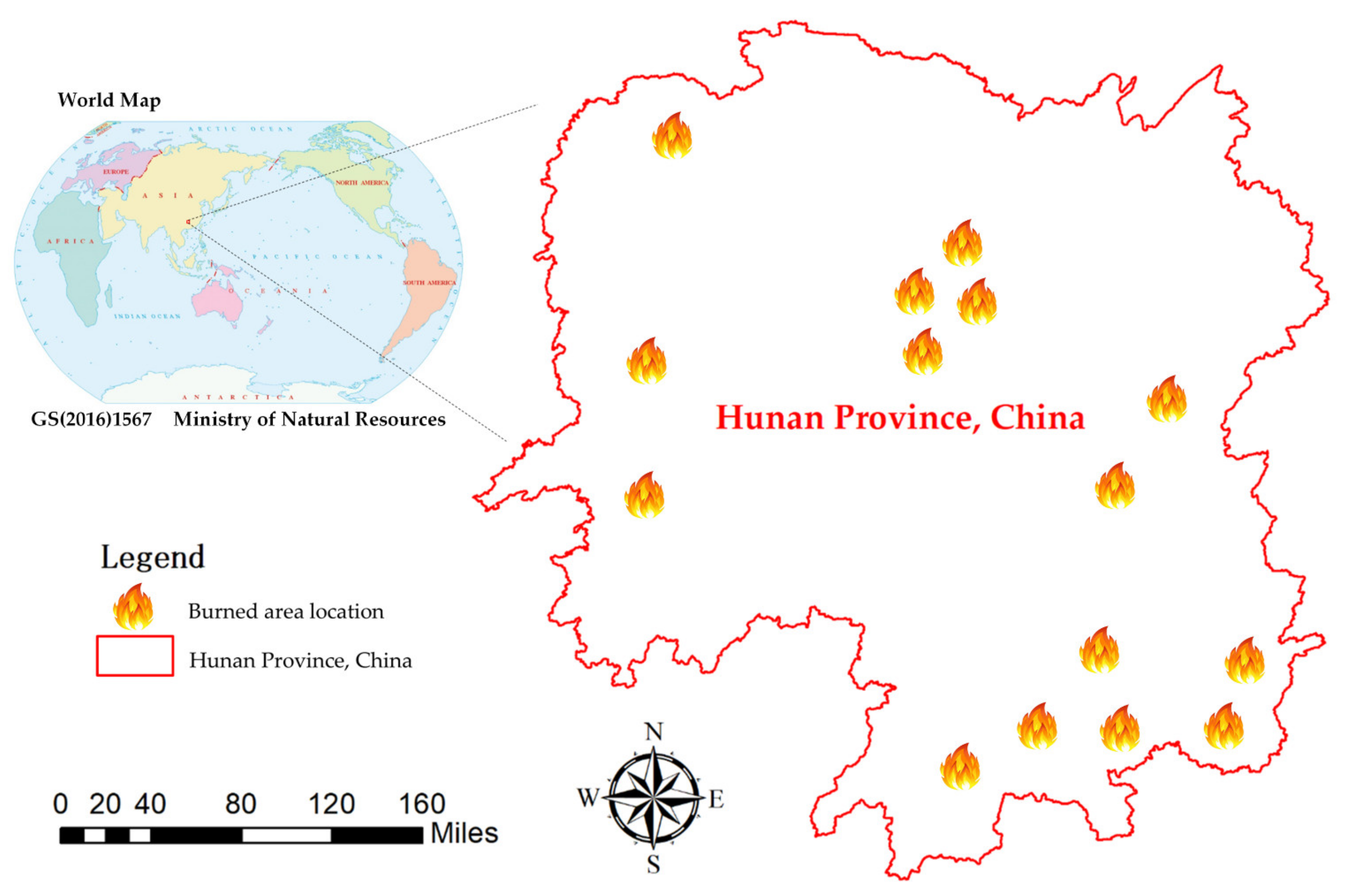
2. Study Area
3. Methodology
3.1. Satellite Data and Preprocessing
3.1.1. Satellite Data
3.1.2. Data Preprocessing
- (1)
- (2)
- (1)
- (2)
- (3)
- (4)
3.2. True Fire-Scar Information
3.3. BASM Approach for Fire Scar Detection
3.3.1. Fully Constrained Least Squares (FCLS)
3.3.2. Modified Pixel Swapping Algorithm (MPSA)
3.4. Accuracy Assessment
4. Results
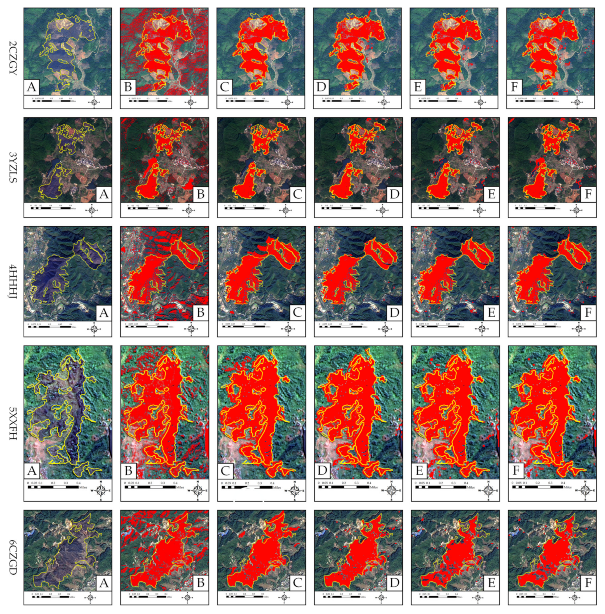
4.1. Reduction of Misclassification Due to Noise
4.2. Pixel and Subpixel Mapping of Burned Area
4.3. Accuracy Assessment of the BASM Approach
5. Discussion
6. Conclusions
Author Contributions
Funding
Data Availability Statement
Conflicts of Interest
References
- Matin, M.A.; Chitale, V.S.; Murthy, M.S.R.; Uddin, K.; Bajracharya, B.; Pradhan, S. Understanding forest fire patterns and risk in Nepal using remote sensing, geographic information system and historical fire data. Int. J. Wildland Fire 2017, 26, 276–286. [Google Scholar] [CrossRef] [Green Version]
- Fernandez-Carrillo, A.; McCaw, L.; Tanase, M.A. Estimating prescribed fire impacts and post-fire tree survival in eucalyptus forests of Western Australia with L-band SAR data. Remote Sens. Environ. 2019, 224, 133–144. [Google Scholar] [CrossRef]
- Sannigrahi, S.; Pilla, F.; Basu, B.; Basu, A.S.; Sarkar, K.; Chakraborti, S.; Joshi, P.K.; Zhang, Q.; Wang, Y.; Bhatt, S.; et al. Examining the effects of forest fire on terrestrial carbon emission and ecosystem production in India using remote sensing approaches. Sci. Total Environ. 2020, 725, 138331. [Google Scholar] [CrossRef] [PubMed]
- Schroeder, W.; Oliva, P.; Giglio, L.; Quayle, B.; Lorenz, E.; Morelli, F. Active fire detection using Landsat-8/OLI data. Remote Sens. Environ. 2016, 185, 210–220. [Google Scholar] [CrossRef] [Green Version]
- Syphard, A.D.; Keeley, J.E. Location, timing and extent of wildfire vary by cause of ignition. Int. J. Wildland Fire 2015, 24, 37–47. [Google Scholar] [CrossRef] [Green Version]
- Zhang, Q.; Ge, L.; Zhang, R.; Metternicht, G.I.; Du, Z.; Kuang, J.; Xu, M. Deep-learning-based burned area mapping using the synergy of Sentinel-1&2 data. Remote Sens. Environ. 2021, 264, 112575. [Google Scholar] [CrossRef]
- National Forest Fire Prevention Plan (2016–2025). 2016. Available online: https://leap.unep.org/countries/cn/national-legislation/national-forest-fire-prevention-plan-2016-2025 (accessed on 4 April 2022).
- Pinto, M.; Trigo, R.; Trigo, I.; DaCamara, C. A Practical Method for High-Resolution Burned Area Monitoring Using Sentinel-2 and VIIRS. Remote Sens. 2021, 13, 1608. [Google Scholar] [CrossRef]
- Daldegan, G.A.; Roberts, D.A.; Ribeiro, F.D.F. Spectral mixture analysis in Google Earth Engine to model and delineate fire scars over a large extent and a long time-series in a rainforest-savanna transition zone. Remote Sens. Environ. 2019, 232. [Google Scholar] [CrossRef]
- Mouillot, F.; Field, C.B. Fire history and the global carbon budget: A 1ox 1o fire history reconstruction for the 20th century. Glob. Chang. Biol. 2005, 11, 398–420. [Google Scholar] [CrossRef]
- Ba, R.; Song, W.; Li, X.; Xie, Z.; Lo, S. Integration of Multiple Spectral Indices and a Neural Network for Burned Area Mapping Based on MODIS Data. Remote Sens. 2019, 11, 326. [Google Scholar] [CrossRef] [Green Version]
- Chuvieco, E.; Mouillot, F.; van der Werf, G.R.; San Miguel, J.; Tanase, M.; Koutsias, N.; García, M.; Yebra, M.; Padilla, M.; Gitas, I.; et al. Historical background and current developments for mapping burned area from satellite Earth observation. Remote Sens. Environ. 2019, 225, 45–64. [Google Scholar] [CrossRef]
- Xie, Z.; Song, W.; Ba, R.; Li, X.; Xia, L. A Spatiotemporal Contextual Model for Forest Fire Detection Using Himawari-8 Satellite Data. Remote Sens. 2018, 10, 1992. [Google Scholar] [CrossRef] [Green Version]
- Florath, J.; Keller, S. Supervised Machine Learning Approaches on Multispectral Remote Sensing Data for a Combined Detec-tion of Fire and Burned Area. Remote Sens. 2022, 14, 657. [Google Scholar] [CrossRef]
- Stroppiana, D.; Bordogna, G.; Sali, M.; Boschetti, M.; Sona, G.; Brivio, P.A. A Fully Automatic, Interpretable and Adaptive Machine Learning Approach to Map Burned Area from Remote Sensing. ISPRS Int. J. Geo-Information 2021, 10, 546. [Google Scholar] [CrossRef]
- Santos, F.L.; Libonati, R.; Peres, L.F.; Pereira, A.A.; Narcizo, L.C.; Rodrigues, J.A.; Oom, D.; Pereira, J.M.C.; Schroeder, W.; Setzer, A.W. Assessing VIIRS capabilities to improve burned area mapping over the Brazilian Cerrado. Int. J. Remote Sens. 2020, 41, 8300–8327. [Google Scholar] [CrossRef]
- Ramo, R.; García, M.; Rodríguez, D.; Chuvieco, E. A data mining approach for global burned area mapping. Int. J. Appl. Earth Obs. Geoinf. ITC J. 2018, 73, 39–51. [Google Scholar] [CrossRef]
- Valencia, G.; Anaya, J.; Velásquez, E.A.; Ramo, R.; Caro-Lopera, F. About Validation-Comparison of Burned Area Products. Remote Sens. 2020, 12, 3972. [Google Scholar] [CrossRef]
- Moreno-Ruiz, J.A.; García-Lázaro, J.R.; Arbelo, M.; Cantón-Garbín, M. MODIS Sensor Capability to Burned Area Mapping—Assessment of Performance and Improvements Provided by the Latest Standard Products in Boreal Regions. Sensors 2020, 20, 5423. [Google Scholar] [CrossRef]
- Otón, G.; Lizundia-Loiola, J.; Pettinari, M.L.; Chuvieco, E. Development of a consistent global long-term burned area product (1982–2018) based on AVHRR-LTDR data. Int. J. Appl. Earth Obs. Geoinf. ITC J. 2021, 103, 102473. [Google Scholar] [CrossRef]
- Zhang, S.; Zhao, H.; Wu, Z.; Tan, L. Comparing the Ability of Burned Area Products to Detect Crop Residue Burning in China. Remote Sens. 2022, 14, 693. [Google Scholar] [CrossRef]
- Humber, M.; Boschetti, L.; Giglio, L.; Justice, C.O. Spatial and temporal intercomparison of four global burned area products. Int. J. Digit. Earth 2018, 12, 460–484. [Google Scholar] [CrossRef]
- Artés, T.; Oom, D.; De Rigo, D.; Durrant, T.H.; Maianti, P.; Libertà, G.; San-Miguel-Ayanz, J. A global wildfire dataset for the analysis of fire regimes and fire behaviour. Sci. Data 2019, 6, 1–11. [Google Scholar] [CrossRef]
- Long, T.; Zhang, Z.; He, G.; Jiao, W.; Tang, C.; Wu, B.; Zhang, X.; Wang, G.; Yin, R. 30 m Resolution Global Annual Burned Area Mapping Based on Landsat Images and Google Earth Engine. Remote Sens. 2019, 11, 489. [Google Scholar] [CrossRef] [Green Version]
- Hawbaker, T.J.; Vanderhoof, M.K.; Schmidt, G.L.; Beal, Y.-J.; Picotte, J.J.; Takacs, J.D.; Falgout, J.T.; Dwyer, J.L. The Landsat Burned Area algorithm and products for the conterminous United States. Remote Sens. Environ. 2020, 244, 111801. [Google Scholar] [CrossRef]
- Pessôa, A.; Anderson, L.; Carvalho, N.; Campanharo, W.; Junior, C.; Rosan, T.; Reis, J.; Pereira, F.; Assis, M.; Jacon, A.; et al. Intercomparison of Burned Area Products and Its Implication for Carbon Emission Estimations in the Amazon. Remote Sens. 2020, 12, 3864. [Google Scholar] [CrossRef]
- Diniz, C.G.; Souza, A.A.D.A.; Santos, D.C.; Dias, M.C.; da Luz, N.C.; de Moraes, D.R.V.; Maia, J.S.A.; Gomes, A.R.; Narvaes, I.D.S.; Valeriano, D.M.; et al. DETER-B: The New Amazon Near Real-Time Deforestation Detection System. IEEE J. Sel. Top. Appl. Earth Obs. Remote Sens. 2015, 8, 3619–3628. [Google Scholar] [CrossRef]
- Andela, N.; Morton, D.C.; Giglio, L.; Paugam, R.; Chen, Y.; Hantson, S.; van der Werf, G.R.; Randerson, J.T. The Global Fire Atlas of individual fire size, duration, speed and direction. Earth Syst. Sci. Data 2019, 11, 529–552. [Google Scholar] [CrossRef] [Green Version]
- Xulu, S.; Mbatha, N.; Peerbhay, K. Burned Area Mapping over the Southern Cape Forestry Region, South Africa Using Sentinel Data within GEE Cloud Platform. ISPRS Int. J. Geo-Information 2021, 10, 511. [Google Scholar] [CrossRef]
- Seydi, S.T.; Hasanlou, M.; Chanussot, J. DSMNN-Net: A Deep Siamese Morphological Neural Network Model for Burned Area Mapping Using Multispectral Sentinel-2 and Hyperspectral PRISMA Images. Remote Sens. 2021, 13, 5138. [Google Scholar] [CrossRef]
- Wang, Q.; Zhang, C.; Atkinson, P.M. Sub-pixel mapping with point constraints. Remote Sens. Environ. 2020, 244, 111817. [Google Scholar] [CrossRef]
- Wu, S.; Ren, J.; Chen, Z.; Jin, W.; Liu, X.; Li, H.; Pan, H.; Guo, W. Influence of reconstruction scale, spatial resolution and pixel spatial relationships on the sub-pixel mapping accuracy of a double-calculated spatial attraction model. Remote Sens. Environ. 2018, 210, 345–361. [Google Scholar] [CrossRef]
- Yu, W.; Li, J.; Liu, Q.; Zeng, Y.; Zhao, J.; Xu, B.; Yin, G. Global Land Cover Heterogeneity Characteristics at Moderate Resolution for Mixed Pixel Modeling and Inversion. Remote Sens. 2018, 10, 856. [Google Scholar] [CrossRef] [Green Version]
- Chen, X.; Wang, D.; Chen, J.; Wang, C.; Shen, M. The mixed pixel effect in land surface phenology: A simulation study. Remote Sens. Environ. 2018, 211, 338–344. [Google Scholar] [CrossRef]
- Daniel, C.; Heinz, C.-I.C. Fully Constrained Least Squares Linear Spectral Mixture Analysis Method for Material Quantification in Hyperspectral Imagery. IEEE Trans. Geosci. Remote Sens. 2001, 39, 529–545. [Google Scholar]
- Shao, Y.; Lan, J. A Spectral Unmixing Method by Maximum Margin Criterion and Derivative Weights to Address Spectral Variability in Hyperspectral Imagery. Remote Sens. 2019, 11, 1045. [Google Scholar] [CrossRef] [Green Version]
- Craig, M. Minimum-volume transforms for remotely sensed data. IEEE Trans. Geosci. Remote Sens. 1994, 32, 542–552. [Google Scholar] [CrossRef]
- Nascimento, J.; Dias, J. Vertex component analysis: A fast algorithm to unmix hyperspectral data. IEEE Trans. Geosci. Remote Sens. 2005, 43, 898–910. [Google Scholar] [CrossRef] [Green Version]
- Chang, C.-I.; Wu, C.-C.; Liu, W.; Ouyang, Y.-C. A New Growing Method for Simplex-Based Endmember Extraction Algorithm. IEEE Trans. Geosci. Remote Sens. 2006, 44, 2804–2819. [Google Scholar] [CrossRef]
- Miao, L.; Qi, H. Endmember Extraction from Highly Mixed Data Using Minimum Volume Constrained Nonnegative Matrix Factorization. IEEE Trans. Geosci. Remote Sens. 2007, 45, 765–777. [Google Scholar] [CrossRef]
- Zhang, J.; Rivard, B.; Rogge, D.M. The Successive Projection Algorithm (SPA), an Algorithm with a Spatial Constraint for the Automatic Search of Endmembers in Hyperspectral Data. Sensors 2008, 8, 1321–1342. [Google Scholar] [CrossRef] [Green Version]
- He, Y.; Yang, J.; Guo, X. Green Vegetation Cover Dynamics in a Heterogeneous Grassland: Spectral Unmixing of Landsat Time Series from 1999 to 2014. Remote Sens. 2020, 12, 3826. [Google Scholar] [CrossRef]
- Winter, M.E. N-FINDR: An Algorithm for Fast Autonomous Spectral End_Member Determination in Hyperspectral Data. In Imaging Spectrom V; International Society for Optics and Photonics: Bellingham, WA, USA, 1999; Volume 3753, pp. 266–275. [Google Scholar] [CrossRef]
- Kumar, U.; Ganguly, S.; Nemani, R.R.; Raja, K.S.; Milesi, C.; Sinha, R.; Michaelis, A.; Votava, P.; Hashimoto, H.; Li, S.; et al. Exploring Subpixel Learning Algorithms for Estimating Global Land Cover Fractions from Satellite Data Using High Performance Computing. Remote Sens. 2017, 9, 1105. [Google Scholar] [CrossRef] [Green Version]
- Atkinson, P.M. Mapping sub-pixel boundaries from remotely sensed images. In Innovations in GIS; Kemp, Z., Ed.; Taylor and Francis: London, UK, 1997; Volume 4, pp. 166–180. [Google Scholar]
- Atkinson, P.M.; Cutler, M.E.J.; Lewis, H. Mapping sub-pixel proportional land cover with AVHRR imagery. Int. J. Remote Sens. 1997, 18, 917–935. [Google Scholar] [CrossRef]
- Atkinson, P.M. Sub-pixel Target Mapping from Soft-classified, Remotely Sensed Imagery. Photogramm. Eng. Remote Sens. 2005, 71, 839–846. [Google Scholar] [CrossRef] [Green Version]
- Wang, Q.; Atkinson, P.M. The effect of the point spread function on sub-pixel mapping. Remote Sens. Environ. 2017, 193, 127–137. [Google Scholar] [CrossRef] [Green Version]
- Wang, Y.; Chen, Q.; Ding, M.; Li, J. High Precision Dimensional Measurement with Convolutional Neural Network and Bi-Directional Long Short-Term Memory (LSTM). Sensors 2019, 19, 5302. [Google Scholar] [CrossRef] [Green Version]
- Hu, C. A novel ocean color index to detect floating algae in the global oceans. Remote Sens. Environ. 2009, 113, 2118–2129. [Google Scholar] [CrossRef]
- Salomonson, V.V.; Appel, I. Estimating fractional snow cover from MODIS using the normalized difference snow index. Remote Sens. Environ. 2004, 89, 351–360. [Google Scholar] [CrossRef]
- Salomonson, V.; Appel, I. Development of the Aqua MODIS NDSI fractional snow cover algorithm and validation results. IEEE Trans. Geosci. Remote Sens. 2006, 44, 1747–1756. [Google Scholar] [CrossRef]
- He, Y.; Chen, G.; Potter, C.; Meentemeyer, R.K. Integrating multi-sensor remote sensing and species distribution modeling to map the spread of emerging forest disease and tree mortality. Remote Sens. Environ. 2019, 231, 111238. [Google Scholar] [CrossRef]
- Li, L.; Chen, Y.; Xu, T.; Shi, K.; Liu, R.; Huang, C.; Lu, B.; Meng, L. Remote Sensing of Wetland Flooding at a Sub-Pixel Scale Based on Random Forests and Spatial Attraction Models. Remote Sens. 2019, 11, 1231. [Google Scholar] [CrossRef] [Green Version]
- Li, X.; Chen, R.; Foody, G.M.; Wang, L.; Yang, X.; Du, Y.; Ling, F. Spatio-Temporal Sub-Pixel Land Cover Mapping of Remote Sensing Imagery Using Spatial Distribution Information from Same-Class Pixels. Remote Sens. 2020, 12, 503. [Google Scholar] [CrossRef] [Green Version]
- Ling, F.; Li, X.; Foody, G.M.; Boyd, D.; Ge, Y.; Li, X.; Du, Y. Monitoring surface water area variations of reservoirs using daily MODIS images by exploring sub-pixel information. ISPRS J. Photogramm. Remote Sens. 2020, 168, 141–152. [Google Scholar] [CrossRef]
- Deng, C.; Zhu, Z. Continuous subpixel monitoring of urban impervious surface using Landsat time series. Remote Sens. Environ. 2018, 238, 110929. [Google Scholar] [CrossRef]
- Ling, F.; Du, Y.; Zhang, Y.; Li, X.; Xiao, F. Burned-Area Mapping at the Subpixel Scale with MODIS Images. IEEE Geosci. Remote Sens. Lett. 2015, 12, 1963–1967. [Google Scholar] [CrossRef]
- Msellmi, B.; Picone, D.; Rabah, Z.; Mura, M.; Farah, I. Sub-Pixel Mapping Model Based on Total Variation Regularization and Learned Spatial Dictionary. Remote Sens. 2021, 13, 190. [Google Scholar] [CrossRef]
- Zhang, C.; Ma, L.; Chen, J.; Rao, Y.; Zhou, Y.; Chen, X. Assessing the impact of endmember variability on linear Spectral Mixture Analysis (LSMA): A theoretical and simulation analysis. Remote Sens. Environ. 2019, 235, 111471. [Google Scholar] [CrossRef]
- Drusch, M.; Del Bello, U.; Carlier, S.; Colin, O.; Fernandez, V.; Gascon, F.; Hoersch, B.; Isola, C.; Laberinti, P.; Martimort, P.; et al. Sentinel-2: ESA’s Optical High-Resolution Mission for GMES Operational Services. Remote Sens. Environ. 2012, 120, 25–36. [Google Scholar] [CrossRef]
- Roteta, E.; Bastarrika, A.; Padilla, M.; Storm, T.; Chuvieco, E. Development of a Sentinel-2 burned area algorithm: Generation of a small fire database for sub-Saharan Africa. Remote Sens. Environ. 2018, 222, 1–17. [Google Scholar] [CrossRef]
- Yan, L.; Roy, D.P.; Li, Z.; Zhang, H.K.; Huang, H. Sentinel-2A multi-temporal misregistration characterization and an orbit-based sub-pixel registration methodology. Remote Sens. Environ. 2018, 215, 495–506. [Google Scholar] [CrossRef]
- Tong, X.-Y.; Xia, G.-S.; Lu, Q.; Shen, H.; Li, S.; You, S.; Zhang, L. Land-cover classification with high-resolution remote sensing images using transferable deep models. Remote Sens. Environ. 2020, 237, 111322. [Google Scholar] [CrossRef] [Green Version]
- Shi, Y.; Wang, Z.; Liu, L.; Li, C.; Peng, D.; Xiao, P. Improving Estimation of Woody Aboveground Biomass of Sparse Mixed Forest over Dryland Ecosystem by Combining Landsat-8, GaoFen-2, and UAV Imagery. Remote Sens. 2021, 13, 4859. [Google Scholar] [CrossRef]
- Li, J.; Chen, X.; Tian, L.; Huang, J.; Feng, L. Improved capabilities of the Chinese high-resolution remote sensing satellite GF-1 for monitoring suspended particulate matter (SPM) in inland waters: Radiometric and spatial considerations. ISPRS J. Photogramm. Remote Sens. 2015, 106, 145–156. [Google Scholar] [CrossRef]
- Lu, C.L.; Wang, R.; Yin, H. GF-1 Satellite Remote Sensing Characters. Spacecr. RecoveryRemote Sens. 2014, 35, 67–73. (In Chinese) [Google Scholar]
- Morresi, D.; Marzano, R.; Lingua, E.; Motta, R.; Garbarino, M. Mapping burn severity in the western Italian Alps through phenologically coherent reflectance composites derived from Sentinel-2 imagery. Remote Sens. Environ. 2021, 269, 112800. [Google Scholar] [CrossRef]
- Louis, J.; Debaecker, V.; Pflug, B.; Main-Knorn, M.; Bieniarz, J.; Mueller-Wilm, U.; Cadau, E.; Gascon, F. Sentinel-2 Sen2cor: L2A Processor for Users. 2016. Available online: https://elib.dlr.de/107381/1/LPS2016_sm10_3louis.pdf (accessed on 19 April 2022).
- Ramo, R.; Roteta, E.; Bistinas, I.; Van Wees, D.; Bastarrika, A.; Chuvieco, E.; Van der Werf, G.R. African burned area and fire carbon emissions are strongly impacted by small fires undetected by coarse resolution satellite data. Proc. Natl. Acad. Sci. USA 2021, 118, e2011160118. [Google Scholar] [CrossRef]
- Rasmy, L.; Sebari, I.; Ettarid, M. Automatic Sub-Pixel Co-Registration of Remote Sensing Images Using Phase Correlation and Harris Detector. Remote Sens. 2021, 13, 2314. [Google Scholar] [CrossRef]
- Parker, B.M.; Lewis, T.; Srivastava, S.K. Estimation and evaluation of multi-decadal fire severity patterns using Landsat sensors. Remote Sens. Environ. 2015, 170, 340–349. [Google Scholar] [CrossRef]
- Hall, R.J.; Freeburn, J.T.; De Groot, W.J.; Pritchard, J.M.; Lynham, T.J.; Landry, R. Remote sensing of burn severity: Experience from western Canada boreal fires. Int. J. Wildland Fire 2008, 17, 476–489. [Google Scholar] [CrossRef]
- Papaloukas, C.; Fotiadis, D.I.; Liavas, A.P.; Likas, A.; Michalis, L.K. A knowledge-based technique for automated detection of ischaemic episodes in long duration elect rocard iog rams. Med. Biol. Eng. Comput. 2001, 39, 105–112. [Google Scholar] [CrossRef]
- Vanderhoof, M.K.; Hawbaker, T.J.; Teske, C.; Ku, A.; Noble, J.; Picotte, J. Mapping Wetland Burned Area from Sentinel-2 across the Southeastern United States and Its Contributions Relative to Landsat-8 (2016–2019). Fire 2021, 4, 52. [Google Scholar] [CrossRef]
- Yue, J.; Tian, Q.; Dong, X.; Xu, N. Using broadband crop residue angle index to estimate the fractional cover of vegetation, crop residue, and bare soil in cropland systems. Remote Sens. Environ. 2019, 237, 111538. [Google Scholar] [CrossRef]
- Zhang, X.; Cheng, B.; Chen, J.; Liang, C. High-Resolution Boundary Refined Convolutional Neural Network for Automatic Agricultural Greenhouses Extraction from GaoFen-2 Satellite Imageries. Remote Sens. 2021, 13, 4237. [Google Scholar] [CrossRef]
- Tong, X.; Liu, S.; Weng, Q. Bias-corrected rational polynomial coefficients for high accuracy geo-positioning of QuickBird stereo imagery. ISPRS J. Photogramm. Remote Sens. 2010, 65, 218–226. [Google Scholar] [CrossRef]
- Rabby, Y.W.; Ishtiaque, A.; Rahman, M.S. Evaluating the Effects of Digital Elevation Models in Landslide Susceptibility Mapping in Rangamati District, Bangladesh. Remote Sens. 2020, 12, 2718. [Google Scholar] [CrossRef]
- Shawky, M.; Moussa, A.; Hassan, Q.K.; El-Sheimy, N. Pixel-Based Geometric Assessment of Channel Networks/Orders Derived from Global Spaceborne Digital Elevation Models. Remote Sens. 2019, 11, 235. [Google Scholar] [CrossRef] [Green Version]
- Vivone, G.; Alparone, L.; Chanussot, J.; Mura, M.D.; Garzelli, A.; Licciardi, G.A.; Restaino, R.; Wald, L. A Critical Comparison Among Pansharpening Algorithms. IEEE Trans. Geosci. Remote Sens. 2014, 53, 2565–2586. [Google Scholar] [CrossRef]
- Wu, Y.; Wang, N.; Li, Z.; Chen, A.; Guo, Z.; Qie, Y. The effect of thermal radiation from surrounding terrain on glacier surface temperatures retrieved from remote sensing data: A case study from Qiyi Glacier, China. Remote Sens. Environ. 2019, 231, 111267. [Google Scholar] [CrossRef]
- Guo, L.; Shi, T.; Linderman, M.; Chen, Y.; Zhang, H.; Fu, P. Exploring the Influence of Spatial Resolution on the Digital Mapping of Soil Organic Carbon by Airborne Hyperspectral VNIR Imaging. Remote Sens. 2019, 11, 1032. [Google Scholar] [CrossRef] [Green Version]
- Awada, H.; Ciraolo, G.; Maltese, A.; Provenzano, G.; Hidalgo, M.A.M.; Còrcoles, J.I. Assessing the performance of a large-scale irrigation system by estimations of actual evapotranspiration obtained by Landsat satellite images resampled with cubic convolution. Int. J. Appl. Earth Obs. Geoinf. ITC J. 2018, 75, 96–105. [Google Scholar] [CrossRef]
- Mo, Y.; Yang, X.; Tang, H.; Li, Z. Smoke Detection from Himawari-8 Satellite Data over Kalimantan Island Using Multilayer Perceptrons. Remote Sens. 2021, 13, 3721. [Google Scholar] [CrossRef]
- Banerjee, K.; Krishnan, P.; Mridha, N. Application of thermal imaging of wheat crop canopy to estimate leaf area index under different moisture stress conditions. Biosyst. Eng. 2018, 166, 13–27. [Google Scholar] [CrossRef]
- Heinz, D.; Chang, C.-I.; Althouse, M.L.G. Fully Constrained Least-Squares Based Linear Unmixing. In Proceedings of the IEEE 1999 International Geoscience and Remote Sensing Symposium. IGARSS’99 (Cat. No.99CH36293), Hamburg, Germany, 28 June–2 July 1999; pp. 1401–1403. [Google Scholar]
- Heylen, R.; Burazerovic, D.; Scheunders, P. Fully Constrained Least Squares Spectral Unmixing by Simplex Projection. IEEE Trans. Geosci. Remote Sens. 2011, 49, 4112–4122. [Google Scholar] [CrossRef]
- Plaza, A.; Martinez, P.; Perez, R.; Plaza, J. A Quantitative and Comparative Analysis of Endmember Extraction Algorithms from Hyperspectral Data. IEEE Trans. Geosci. Remote Sens. 2004, 42, 650–663. [Google Scholar] [CrossRef]
- Hamedianfar, A.; Shafri, H.Z.M.; Mansor, S.; Ahmad, N. Improving detailed rule-based feature extraction of urban areas from WorldView-2 image and lidar data. Int. J. Remote Sens. 2014, 35, 1876–1899. [Google Scholar] [CrossRef]
- Jahjah, M.; Ulivieri, C. Automatic archaeological feature extraction from satellite VHR images. Acta Astronaut. 2010, 66, 1302–1310. [Google Scholar] [CrossRef]
- Mansaray, L.R.; Yang, L.; Kabba, V.T.; Kanu, A.S.; Huang, J.; Wang, F. Optimising rice mapping in cloud-prone environments by combining quad-source optical with Sentinel-1A microwave satellite imagery. GISci. Remote Sens. 2019, 56, 1333–1354. [Google Scholar] [CrossRef]
- Fetai, B.; Oštir, K.; Kosmatin Fras, M.; Lisec, A. Extraction of Visible Boundaries for Cadastral Mapping Based on UAV Imagery. Remote Sens. 2019, 11, 1510. [Google Scholar] [CrossRef] [Green Version]
- Huang, G.; Yan, B.; Mou, Z.; Wu, K.; Lv, X. Surrogate Model for Torsional Behavior of Bundle Conductors and its Application. IEEE Trans. Power Deliv. 2021, 37, 67–75. [Google Scholar] [CrossRef]
- Bisoyi, N.; Gupta, H.; Padhy, N.P.; Chakrapani, G.J. Prediction of daily sediment discharge using a back propagation neural network training algorithm: A case study of the Narmada River, India. Int. J. Sediment Res. 2018, 34, 125–135. [Google Scholar] [CrossRef]
- Nedaie, A.; Najafi, A.A. Support vector machine with Dirichlet feature mapping. Neural Networks 2018, 98, 87–101. [Google Scholar] [CrossRef]
- Hamilton, D.; Brothers, K.; McCall, C.; Gautier, B.; Shea, T. Mapping Forest Burn Extent from Hyperspatial Imagery Using Machine Learning. Remote Sens. 2021, 13, 3843. [Google Scholar] [CrossRef]
- Zhan, P.; Zhu, W.; Li, N. An automated rice mapping method based on flooding signals in synthetic aperture radar time series. Remote Sens. Environ. 2020, 252, 112112. [Google Scholar] [CrossRef]
- Sebald, J.; Senf, C.; Seidl, R. Human or natural? Landscape context improves the attribution of forest disturbances mapped from Landsat in Central Europe. Remote Sens. Environ. 2021, 262, 112502. [Google Scholar] [CrossRef]
- Nelson, M.D.; Garner, J.D.; Tavernia, B.G.; Stehman, S.V.; Riemann, R.I.; Lister, A.J.; Perry, C.H. Assessing map accuracy from a suite of site-specific, non-site specific, and spatial distribution approaches. Remote Sens. Environ. 2021, 260. [Google Scholar] [CrossRef]
- Ji, C.; Bachmann, M.; Esch, T.; Feilhauer, H.; Heiden, U.; Heldens, W.; Hueni, A.; Lakes, T.; Metz-Marconcini, A.; Schroedter-Homscheidt, M.; et al. Solar photovoltaic module detection using laboratory and airborne imaging spectroscopy data. Remote Sens. Environ. 2021, 266, 112692. [Google Scholar] [CrossRef]
- Watanabe, M.; Koyama, C.N.; Hayashi, M.; Nagatani, I.; Tadono, T.; Shimada, M. Refined algorithm for forest early warning system with ALOS-2/PALSAR-2 ScanSAR data in tropical forest regions. Remote Sens. Environ. 2021, 265, 112643. [Google Scholar] [CrossRef]
- Foody, G.M. Impacts of ignorance on the accuracy of image classification and thematic mapping. Remote Sens. Environ. 2021, 259, 112367. [Google Scholar] [CrossRef]
- Wu, X.; Shi, Z.; Zou, Z. A geographic information-driven method and a new large scale dataset for remote sensing cloud/snow detection. ISPRS J. Photogramm. Remote Sens. 2021, 174, 87–104. [Google Scholar] [CrossRef]
- Hao, Z.; Lin, L.; Post, C.J.; Mikhailova, E.A.; Li, M.; Chen, Y.; Yu, K.; Liu, J. Automated tree-crown and height detection in a young forest plantation using mask region-based convolutional neural network (Mask R-CNN). ISPRS J. Photogramm. Remote Sens. 2021, 178, 112–123. [Google Scholar] [CrossRef]
- Jiang, Z.; Zhang, J.; Ma, Y.; Mao, X. Hyperspectral Remote Sensing Detection of Marine Oil Spills Using an Adaptive Long-Term Moment Estimation Optimizer. Remote Sens. 2021, 14, 157. [Google Scholar] [CrossRef]
- Bhattarai, R.; Rahimzadeh-Bajgiran, P.; Weiskittel, A.; Meneghini, A.; MacLean, D.A. Spruce budworm tree host species distribution and abundance mapping using multi-temporal Sentinel-1 and Sentinel-2 satellite imagery. ISPRS J. Photogramm. Remote Sens. 2020, 172, 28–40. [Google Scholar] [CrossRef]
- Hu, X.; Ban, Y.; Nascetti, A. Uni-Temporal Multispectral Imagery for Burned Area Mapping with Deep Learning. Remote Sens. 2021, 13, 1509. [Google Scholar] [CrossRef]
- Mouillot, F.; Schultz, M.G.; Yue, C.; Cadule, P.; Tansey, K.; Ciais, P.; Chuvieco, E. Ten years of global burned area products from spaceborne remote sensing—A review: Analysis of user needs and recommendations for future developments. Int. J. Appl. Earth Obs. Geoinf. 2014, 26, 64–79. [Google Scholar] [CrossRef] [Green Version]
- Mangeon, S.; Field, R.; Fromm, M.; McHugh, C.; Voulgarakis, A. Satellite versus ground-based estimates of burned area: A comparison between MODIS based burned area and fire agency reports over North America in 2007. Anthr. Rev. 2015, 3, 76–92. [Google Scholar] [CrossRef] [Green Version]
- Chang, Y.; Yan, L.; Fang, H.; Liu, H. Simultaneous Destriping and Denoising for Remote Sensing Images With Unidirectional Total Variation and Sparse Representation. IEEE Geosci. Remote Sens. Lett. 2013, 11, 1051–1055. [Google Scholar] [CrossRef]
- Ebadi, L.; Shafri, H.Z.M.; Mansor, S.B.; Ashurov, R. A review of applying second-generation wavelets for noise removal from remote sensing data. Environ. Earth Sci. 2013, 70, 2679–2690. [Google Scholar] [CrossRef] [Green Version]
- Ha, C.; Kim, W.; Jeong, J. Remote sensing image enhancement based on singular value decomposition. Opt. Eng. 2013, 52, 083101. [Google Scholar] [CrossRef]
- Hird, J.N.; McDermid, G.J. Noise reduction of NDVI time series: An empirical comparison of selected techniques. Remote Sens. Environ. 2009, 113, 248–258. [Google Scholar] [CrossRef]
- Gajardo, J.; Mora, M.; Valdés-Nicolao, G.; Carrasco-Benavides, M. Burned Area Classification Based on Extreme Learning Machine and Sentinel-2 Images. Appl. Sci. 2021, 12, 9. [Google Scholar] [CrossRef]
- Knopp, L.; Wieland, M.; Rättich, M.; Martinis, S. A Deep Learning Approach for Burned Area Segmentation with Sentinel-2 Data. Remote Sens. 2020, 12, 2422. [Google Scholar] [CrossRef]
- Ruescas, A.B.; Sobrino, J.A.; Julien, Y.; Jiménez-Muñoz, J.C.; Sòria, G.; Hidalgo, V.; Atitar, M.; Franch, B.; Cuenca, J.; Mattar, C. Mapping sub-pixel burnt percentage using AVHRR data. Application to the Alcalaten area in Spain. Int. J. Remote Sens. 2010, 31, 5315–5330. [Google Scholar] [CrossRef]


| No. | Burned-Area Product | Developer | Sensor | Spatial Resolution | Reference |
|---|---|---|---|---|---|
| 1 | Fire CCI 5.0 | ESA | MODIS | 250 m | [18] |
| 2 | Fire CCI 5.1 | ESA | MODIS | 250 m | [19] |
| 3 | FireCCILT10 | ESA | AVHRR | 0.25° | [20] |
| 4 | Copernicus burnt area | European Commission | PROBA-V | 300 m | [21] |
| 5 | MCD64A1 c6 | NASA | MODIS | 500 m | [22] |
| 6 | GWIS | JRC | MODIS | 500 m | [23] |
| 7 | GABAM | IRSDE/CAS | Landsat 8 OLI | 30 m | [24] |
| 8 | Landsat Burned Area | NASA | Landsat TM Landsat ETM+ Landsat OLI | 30 m | [25] |
| 9 | TREES | TREES-INPE | MODIS | 250 m | [26] |
| 10 | DETER B | INPE | AWiFS | 64 m | [27] |
| 11 | Global Fire Atlas | NASA | MODIS | 500 m | [28] |
| Satellite | Sensor | Band Number | Band Width (μm) | Spatial Resolution (m) |
|---|---|---|---|---|
| Sentinel 2 | MSI | 2 | 0.46–0.52 | 10 |
| 3 | 0.54–0.58 | |||
| 4 | 0.65–0.68 | |||
| 8 | 0.79–0.90 | |||
| GF 1, GF 1B, GF1C, GF1D | PMS | 1 | 0.45–0.90 | 2 |
| 2 | 0.45–0.52 | 8 | ||
| 3 | 0.52–0.59 | |||
| 4 | 0.63–0.69 | |||
| 5 | 0.77–0.89 | |||
| GF 2 | PMS | 1 | 0.45–0.90 | 1 |
| 2 | 0.45–0.52 | 4 | ||
| 3 | 0.52–0.59 | |||
| 4 | 0.63–0.69 | |||
| 5 | 0.77–0.89 |
| No. | Date of the Fire Event | Longitude | Latitude | Extent (ha) |
|---|---|---|---|---|
| 1HYHD | 24 September 2019 | 113°3′ | 27°8′ | 1244.42 |
| 2CZGY | 16 December 2019 | 112°53′ | 25°54′ | 166.82 |
| 3YZLS | 1 October 2019 | 112°8′ | 25°32′ | 95.32 |
| 4HHHJ | 6 October 2018 | 109°53′ | 27°15′ | 87.18 |
| 5XXFH | 6 April 2019 | 109°40′ | 28°2′ | 78.23 |
| 6CZGD | 4 January 2021 | 113°54′ | 25°58′ | 66.61 |
| 7CSNX | 19 March 2020 | 112°0′ | 28°11′ | 53.06 |
| 8CZGY | 31 October 2019 | 112°41′ | 25°29′ | 50.14 |
| 9CZBH | 6 February 2019 | 112°52′ | 25°42′ | 39.18 |
| 10ZZLL | 16 April 2020 | 113°27′ | 27°25′ | 37.99 |
| 11ZJJSZ | 19 March 2020 | 110°0′ | 29°25′ | 34.72 |
| 12CZGD | 19 January 2021 | 113°48′ | 25°49′ | 21.81 |
| 13YYTJ | 9 April 2020 | 111°59′ | 28°16′ | 21.62 |
| 14YYTJ | 9 April 2020 | 112°0′ | 28°16′ | 18.41 |
| 15YYTJ | 14 March 2020 | 111°59′ | 28°14′ | 8.70 |
| Model | Parameter Setup | Training Percent |
|---|---|---|
| FERB |
| - |
| RF |
| 30% |
| BPNN |
| 30% |
| SVM |
| 30% |
| Ground Truth | Burned Area | Background | |
|---|---|---|---|
| Prediction | |||
| Burned area | True Positive (TP) | False Positive (FP) | |
| Background | False Negative (FN) | True Negative (TN) | |
| No. | Algorithm | Ground Truth | Burned Area | Background | OA | UA | PA | IoU | Kappa | |
|---|---|---|---|---|---|---|---|---|---|---|
| Prediction | ||||||||||
| 1HYHD | BASM-FERB | Burned area | 2,026,688 | 159,559 | 98.56% | 92.70% | 94.04% | 87.56% | 92.56% | |
| Background | 128,375 | 17,724,410 | ||||||||
| BASM-RF | Burned area | 2,082,757 | 288,361 | 98.20% | 87.84% | 96.64% | 85.24% | 91.02% | ||
| Background | 72,306 | 17,595,608 | ||||||||
| BASM-BPNN | Burned area | 2,073,524 | 387,511 | 97.66% | 84.25% | 96.22% | 81.55% | 88.52% | ||
| Background | 81,539 | 17,496,458 | ||||||||
| BASM-SVM | Burned area | 2,086,017 | 486,179 | 97.23% | 81.10% | 96.80% | 78.98% | 86.70% | ||
| Background | 69,046 | 17,397,790 | ||||||||
| BASM-notra | Burned area | 2,098,326 | 3,151,184 | 83.99% | 39.97% | 97.37% | 39.54% | 48.88% | ||
| Background | 56,737 | 14,732,785 | ||||||||
| 2CZGY | BASM-FERB | Burned area | 223,195 | 44,697 | 98.08% | 83.32% | 85.82% | 73.24% | 83.53% | |
| Background | 36,866 | 3,939,935 | ||||||||
| BASM-RF | Burned area | 232,539 | 75,721 | 97.57% | 75.44% | 89.42% | 69.25% | 80.54% | ||
| Background | 27,522 | 3,908,911 | ||||||||
| BASM-BPNN | Burned area | 225,850 | 70,289 | 97.54% | 76.26% | 86.85% | 68.37% | 79.90% | ||
| Background | 34,211 | 3,914,343 | ||||||||
| BASM-SVM | Burned area | 230,479 | 92,204 | 97.13% | 71.43% | 88.62% | 65.43% | 77.58% | ||
| Background | 29,582 | 3,892,428 | ||||||||
| BASM-notra | Burned area | 241,068 | 1,343,544 | 67.90% | 15.21% | 92.70% | 15.03% | 17.45% | ||
| Background | 18,993 | 2,641,088 | ||||||||
| 3YZLS | BASM-FERB | Burned area | 200,224 | 57,503 | 98.99% | 77.69% | 88.52% | 70.58% | 82.23% | |
| Background | 25,973 | 7,965,280 | ||||||||
| BASM-RF | Burned area | 205,704 | 145,159 | 97.99% | 58.63% | 90.94% | 55.39% | 70.30% | ||
| Background | 20,493 | 7,877,624 | ||||||||
| BASM-BPNN | Burned area | 205,320 | 192,130 | 97.42% | 51.66% | 90.77% | 49.08% | 64.61% | ||
| Background | 20,877 | 7,830,653 | ||||||||
| BASM-SVM | Burned area | 204,996 | 208,250 | 97.22% | 49.61% | 90.63% | 47.19% | 62.80% | ||
| Background | 21,201 | 7,814,533 | ||||||||
| BASM-notra | Burned area | 205,681 | 1,036,790 | 87.18% | 16.55% | 90.93% | 16.29% | 24.51% | ||
| Background | 20,516 | 6,985,993 | ||||||||
| 4HHHJ | BASM-FERB | Burned area | 184,576 | 26,509 | 96.26% | 87.44% | 86.30% | 76.78% | 84.68% | |
| Background | 29,306 | 1,250,957 | ||||||||
| BASM-RF | Burned area | 184,338 | 12,439 | 97.18% | 93.68% | 86.19% | 81.45% | 88.15% | ||
| Background | 29,544 | 1,265,027 | ||||||||
| BASM-BPNN | Burned area | 183,598 | 20,268 | 96.61% | 90.06% | 85.84% | 78.41% | 85.93% | ||
| Background | 30,284 | 1,257,198 | ||||||||
| BASM-SVM | Burned area | 185,900 | 18,787 | 96.86% | 90.82% | 86.92% | 79.90% | 87.00% | ||
| Background | 27,982 | 1,258,679 | ||||||||
| BASM-notra | Burned area | 187,594 | 272,474 | 79.97% | 40.78% | 87.71% | 38.57% | 44.88% | ||
| Background | 26,288 | 1,004,992 | ||||||||
| 5XXFH | BASM-FERB | Burned area | 128,313 | 50,831 | 92.08% | 71.63% | 95.19% | 69.13% | 76.82% | |
| Background | 6478 | 537,928 | ||||||||
| BASM-RF | Burned area | 128,592 | 55,431 | 91.48% | 69.88% | 95.40% | 67.60% | 75.37% | ||
| Background | 6199 | 533,328 | ||||||||
| BASM-BPNN | Burned area | 128,266 | 59,456 | 90.88% | 68.33% | 95.16% | 66.03% | 73.88% | ||
| Background | 6525 | 529,303 | ||||||||
| BASM-SVM | Burned area | 128,461 | 57,418 | 91.19% | 69.11% | 95.30% | 66.83% | 74.64% | ||
| Background | 6330 | 531,341 | ||||||||
| BASM-notra | Burned area | 129,416 | 147,370 | 78.89% | 46.76% | 96.01% | 45.87% | 50.48% | ||
| Background | 5375 | 441,389 | ||||||||
| 6CZGD | BASM-FERB | Burned area | 113,575 | 61,535 | 98.78% | 64.86% | 83.72% | 57.60% | 72.48% | |
| Background | 22,081 | 6,641,201 | ||||||||
| BASM-RF | Burned area | 108,901 | 149,392 | 97.42% | 42.16% | 80.28% | 38.20% | 54.09% | ||
| Background | 26,755 | 6,553,344 | ||||||||
| BASM-BPNN | Burned area | 86,921 | 100,463 | 97.82% | 46.39% | 64.07% | 36.81% | 52.73% | ||
| Background | 48,735 | 6,602,273 | ||||||||
| BASM-SVM | Burned area | 90,620 | 169,078 | 96.87% | 34.89% | 66.80% | 29.74% | 44.39% | ||
| Background | 45,036 | 6,533,658 | ||||||||
| BASM-notra | Burned area | 117,067 | 2,076,082 | 69.37% | 5.34% | 86.30% | 5.29% | 6.56% | ||
| Background | 18,589 | 4,626,654 | ||||||||
| 7CSNX | BASM-FERB | Burned area | 105,881 | 9985 | 99.28% | 91.38% | 89.65% | 82.66% | 90.13% | |
| Background | 12,225 | 2,968,290 | ||||||||
| BASM-RF | Burned area | 105,414 | 24,109 | 98.81% | 81.39% | 89.25% | 74.12% | 84.52% | ||
| Background | 12,692 | 2,954,166 | ||||||||
| BASM-BPNN | Burned area | 101,541 | 39,733 | 98.18% | 71.88% | 85.97% | 64.33% | 77.35% | ||
| Background | 16,565 | 2,938,542 | ||||||||
| BASM-SVM | Burned area | 104,017 | 60,100 | 97.60% | 63.38% | 88.07% | 58.37% | 72.49% | ||
| Background | 14,089 | 2,918,175 | ||||||||
| BASM-notra | Burned area | 106,945 | 776,466 | 74.56% | 12.11% | 90.55% | 11.95% | 15.68% | ||
| Background | 11,161 | 2,201,809 | ||||||||
| 8CZGY | BASM-FERB | Burned area | 109,602 | 18,969 | 99.78% | 85.25% | 91.69% | 79.14% | 88.24% | |
| Background | 9927 | 12,827,564 | ||||||||
| BASM-RF | Burned area | 106,355 | 70,008 | 99.36% | 60.30% | 88.98% | 56.11% | 71.58% | ||
| Background | 13,174 | 12,776,525 | ||||||||
| BASM-BPNN | Burned area | 91,376 | 101,001 | 99.00% | 47.50% | 76.45% | 41.43% | 58.12% | ||
| Background | 28,153 | 12,745,532 | ||||||||
| BASM-SVM | Burned area | 92,605 | 148,864 | 98.64% | 38.35% | 77.47% | 34.50% | 50.70% | ||
| Background | 26,924 | 12,697,669 | ||||||||
| BASM-notra | Burned area | 110,832 | 3,116,582 | 75.90% | 3.43% | 92.72% | 3.42% | 4.93% | ||
| Background | 8697 | 9,729,951 | ||||||||
| 9CZBH | BASM-FERB | Burned area | 79,646 | 6466 | 99.71% | 92.49% | 84.23% | 78.84% | 88.02% | |
| Background | 14,909 | 7,253,485 | ||||||||
| BASM-RF | Burned area | 81,599 | 132,326 | 98.02% | 38.14% | 86.30% | 35.97% | 52.05% | ||
| Background | 12,956 | 7,127,625 | ||||||||
| BASM-BPNN | Burned area | 80,102 | 33,232 | 99.35% | 70.68% | 84.71% | 62.68% | 76.74% | ||
| Background | 14,453 | 7,226,719 | ||||||||
| BASM-SVM | Burned area | 80,723 | 69,095 | 98.87% | 53.88% | 85.37% | 49.33% | 65.52% | ||
| Background | 13,832 | 7,190,856 | ||||||||
| BASM-notra | Burned area | 81,637 | 1,361,640 | 81.31% | 5.66% | 86.34% | 5.61% | 8.41% | ||
| Background | 12,918 | 5,898,311 | ||||||||
| 10ZZLL | BASM-FERB | Burned area | 79,636 | 21,504 | 98.54% | 78.74% | 96.34% | 76.45% | 85.89% | |
| Background | 3027 | 1,575,007 | ||||||||
| BASM-RF | Burned area | 80,329 | 31,448 | 97.99% | 71.87% | 97.18% | 70.40% | 81.58% | ||
| Background | 2334 | 1,565,063 | ||||||||
| BASM-BPNN | Burned area | 79,095 | 43,596 | 97.19% | 64.47% | 95.68% | 62.65% | 75.60% | ||
| Background | 3568 | 1,552,915 | ||||||||
| BASM-SVM | Burned area | 79,949 | 35,429 | 97.73% | 69.29% | 96.72% | 67.70% | 79.57% | ||
| Background | 2714 | 1,561,082 | ||||||||
| BASM-notra | Burned area | 80,789 | 415,268 | 75.16% | 16.29% | 97.73% | 16.22% | 21.28% | ||
| Background | 1874 | 1,181,243 | ||||||||
| 11ZJJSZ | BASM-FERB | Burned area | 74,445 | 14,469 | 98.81% | 83.73% | 95.12% | 80.28% | 88.44% | |
| Background | 3816 | 1,444,226 | ||||||||
| BASM-RF | Burned area | 76,165 | 33,209 | 97.70% | 69.64% | 97.32% | 68.33% | 80.00% | ||
| Background | 2096 | 1,425,486 | ||||||||
| BASM-BPNN | Burned area | 75,969 | 28,422 | 98.00% | 72.77% | 97.07% | 71.21% | 82.15% | ||
| Background | 2292 | 1,430,273 | ||||||||
| BASM-SVM | Burned area | 76,088 | 42,822 | 97.07% | 63.99% | 97.22% | 62.84% | 75.69% | ||
| Background | 2173 | 1,415,873 | ||||||||
| BASM-notra | Burned area | 76,134 | 358,382 | 76.54% | 17.52% | 97.28% | 17.44% | 23.05% | ||
| Background | 2127 | 1,100,313 | ||||||||
| 12CZGD | BASM-FERB | Burned area | 51,663 | 16,858 | 98.00% | 75.40% | 94.67% | 72.33% | 82.89% | |
| Background | 2909 | 915,928 | ||||||||
| BASM-RF | Burned area | 51,378 | 11,115 | 98.55% | 82.21% | 94.15% | 78.22% | 87.01% | ||
| Background | 3194 | 921,671 | ||||||||
| BASM-BPNN | Burned area | 51,823 | 21,254 | 97.57% | 70.92% | 94.96% | 68.34% | 79.93% | ||
| Background | 2749 | 911,532 | ||||||||
| BASM-SVM | Burned area | 51,871 | 23,054 | 97.39% | 69.23% | 95.05% | 66.82% | 78.75% | ||
| Background | 2701 | 909,732 | ||||||||
| BASM-notra | Burned area | 52,156 | 248,396 | 74.60% | 17.35% | 95.57% | 17.22% | 22.08% | ||
| Background | 2416 | 684,390 | ||||||||
| 13YYTJ | BASM-FERB | Burned area | 56,955 | 7470 | 99.10% | 88.41% | 88.87% | 79.59% | 88.17% | |
| Background | 7133 | 1,553,830 | ||||||||
| BASM-RF | Burned area | 57,249 | 29,067 | 97.79% | 66.32% | 89.33% | 61.46% | 75.00% | ||
| Background | 6839 | 1,532,233 | ||||||||
| BASM-BPNN | Burned area | 54,470 | 46,672 | 96.54% | 53.85% | 84.99% | 49.18% | 64.20% | ||
| Background | 9618 | 1,514,628 | ||||||||
| BASM-SVM | Burned area | 54,566 | 41,569 | 96.86% | 56.76% | 85.14% | 51.64% | 66.53% | ||
| Background | 9522 | 1,519,731 | ||||||||
| BASM-notra | Burned area | 57,299 | 364,515 | 77.16% | 13.58% | 89.41% | 13.37% | 17.97% | ||
| Background | 6789 | 1,196,785 | ||||||||
| 14YYTJ | BASM-FERB | Burned area | 37,597 | 4881 | 98.42% | 88.51% | 76.81% | 69.84% | 81.42% | |
| Background | 11,354 | 975,321 | ||||||||
| BASM-RF | Burned area | 37,398 | 20,004 | 96.93% | 65.15% | 76.40% | 54.24% | 68.72% | ||
| Background | 11,553 | 960,198 | ||||||||
| BASM-BPNN | Burned area | 37,517 | 35,993 | 95.39% | 51.04% | 76.64% | 44.17% | 58.93% | ||
| Background | 11,434 | 944,209 | ||||||||
| BASM-SVM | Burned area | 36,738 | 28,961 | 96.00% | 55.92% | 75.05% | 47.15% | 62.02% | ||
| Background | 12,213 | 951,241 | ||||||||
| BASM-notra | Burned area | 37,882 | 223,392 | 77.22% | 14.50% | 77.39% | 13.91% | 17.84% | ||
| Background | 11,069 | 756,810 | ||||||||
| 15YYTJ | BASM-FERB | Burned area | 17,275 | 9606 | 97.30% | 64.26% | 91.84% | 60.80% | 74.24% | |
| Background | 1534 | 384,615 | ||||||||
| BASM-RF | Burned area | 17,248 | 12,262 | 96.65% | 58.45% | 91.70% | 55.51% | 69.71% | ||
| Background | 1561 | 381,959 | ||||||||
| BASM-BPNN | Burned area | 16,632 | 14,289 | 96.01% | 53.79% | 88.43% | 50.25% | 64.90% | ||
| Background | 2177 | 379,932 | ||||||||
| BASM-SVM | Burned area | 16,938 | 16,300 | 95.60% | 50.96% | 90.05% | 48.24% | 62.93% | ||
| Background | 1871 | 377,921 | ||||||||
| BASM-notra | Burned area | 17,383 | 92,802 | 77.19% | 15.78% | 92.42% | 15.57% | 20.79% | ||
| Background | 1426 | 301,419 | ||||||||
| Average | BASM-FERB | 98.11% | 81.72% | 89.52% | 74.32% | 83.98% | ||||
| BASM-RF | 97.44% | 68.07% | 89.97% | 63.43% | 75.31% | |||||
| BASM-BPNN | 97.01% | 64.92% | 86.92% | 59.63% | 72.23% | |||||
| BASM-SVM | 96.82% | 61.25% | 87.68% | 56.98% | 69.82% | |||||
| BASM-notra | 77.13% | 18.72% | 91.36% | 18.35% | 22.99% | |||||
Publisher’s Note: MDPI stays neutral with regard to jurisdictional claims in published maps and institutional affiliations. |
© 2022 by the authors. Licensee MDPI, Basel, Switzerland. This article is an open access article distributed under the terms and conditions of the Creative Commons Attribution (CC BY) license (https://creativecommons.org/licenses/by/4.0/).
Share and Cite
Xu, H.; Zhang, G.; Zhou, Z.; Zhou, X.; Zhang, J.; Zhou, C. Development of a Novel Burned-Area Subpixel Mapping (BASM) Workflow for Fire Scar Detection at Subpixel Level. Remote Sens. 2022, 14, 3546. https://doi.org/10.3390/rs14153546
Xu H, Zhang G, Zhou Z, Zhou X, Zhang J, Zhou C. Development of a Novel Burned-Area Subpixel Mapping (BASM) Workflow for Fire Scar Detection at Subpixel Level. Remote Sensing. 2022; 14(15):3546. https://doi.org/10.3390/rs14153546
Chicago/Turabian StyleXu, Haizhou, Gui Zhang, Zhaoming Zhou, Xiaobing Zhou, Jia Zhang, and Cui Zhou. 2022. "Development of a Novel Burned-Area Subpixel Mapping (BASM) Workflow for Fire Scar Detection at Subpixel Level" Remote Sensing 14, no. 15: 3546. https://doi.org/10.3390/rs14153546
APA StyleXu, H., Zhang, G., Zhou, Z., Zhou, X., Zhang, J., & Zhou, C. (2022). Development of a Novel Burned-Area Subpixel Mapping (BASM) Workflow for Fire Scar Detection at Subpixel Level. Remote Sensing, 14(15), 3546. https://doi.org/10.3390/rs14153546