Abstract
Groundwater overexploitation is a critical issue in the North China Plain (NCP), resulting in groundwater level decline and surface subsidence for the last half-century. This problem, however, has been greatly alleviated by the South-to-North Water Diversion (SNWD) Project since 2015. Monitoring of this process has been steadily improved in recent years using water level and geodetic observations. Here, we characterize the water storage change at the Huairou groundwater reserve site (HGRS) in Beijing due to the SNWD by combining Interferometric Synthetic Aperture Radar (InSAR) data of the Sentinel-1 satellites, continuous Global Positioning System (GPS) data, and well water level data observed during the same time. InSAR observations revealed subsidence up to ~400 mm in the Beijing plain but uplift at ~40 mm in the HGRS during 2015–2019, and more than 70% of the uplift occurred from October 2018 to January 2019. By integrating the most significant uplift deformation during October 2018 to January 2019 with water level observations at the same time, we estimated the storativity of the confined aquifer system at HGRS as , weighing in the correction for effective stress and surface deformation for various situations. Based on the estimated aquifer storativity and the observed water level change in the unconfined and confined aquifer, the recharged water storage for the confined and unconfined aquifers was estimated as and ~ from 6 October 2018 to 22 January 2019, respectively, which is about 4% and 91% of the surface water recharge through river channels in the same period due to the SNWD Project. Our study demonstrates that integration of geodetic and hydrological data can provide crucial information for the assessment of groundwater circulation and assistance of groundwater management.
1. Introduction
Groundwater is a vital source of fresh water for agriculture, industry, public supply, and ecosystems in many parts of the world. In the North China Plain (NCP), the most important grain production base of China, urban water supplies and agricultural irrigation water rely heavily on groundwater resources. Due to the semi-arid climate, insufficient precipitation, and the development of metropolitan and agriculture areas, the imbalance between the groundwater supply and demand in NCP is conspicuous. In the last decades, more than 50% of the fresh water in NCP has come from the groundwater [1], and groundwater overexploitation in shallow (unconfined) aquifers and deep (confined) aquifers reached ~2.6 and ~1.2 /yr, respectively [2].
The metropolitan Beijing, located in the northwest part of the NCP, also suffers from serious water shortages and large-scale surface subsidence caused by the long-term overexploitation of groundwater. Water resource per capita in Beijing City is , which is far less than the international threshold of for extreme water scarcity [3]. Due to the serious shortage and increasing demand for water resources, the Beijing government constructed the Huairou groundwater reserve site (HGRS) in 2003 [4], which has good hydrological conditions and abundant groundwater storage. The site is located in the alluvial fan of the upper-middle reaches of the Chaobai River and is centered on several rivers in the neighboring region (Figure 1). The HGRS region started to supply groundwater to the urban area in 2003, but it caused a rapid groundwater storage depletion in this region and serious environmental problems, such as land subsidence and ecological degradation, etc.
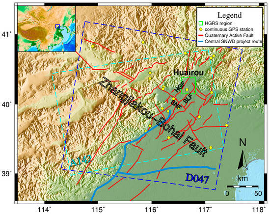
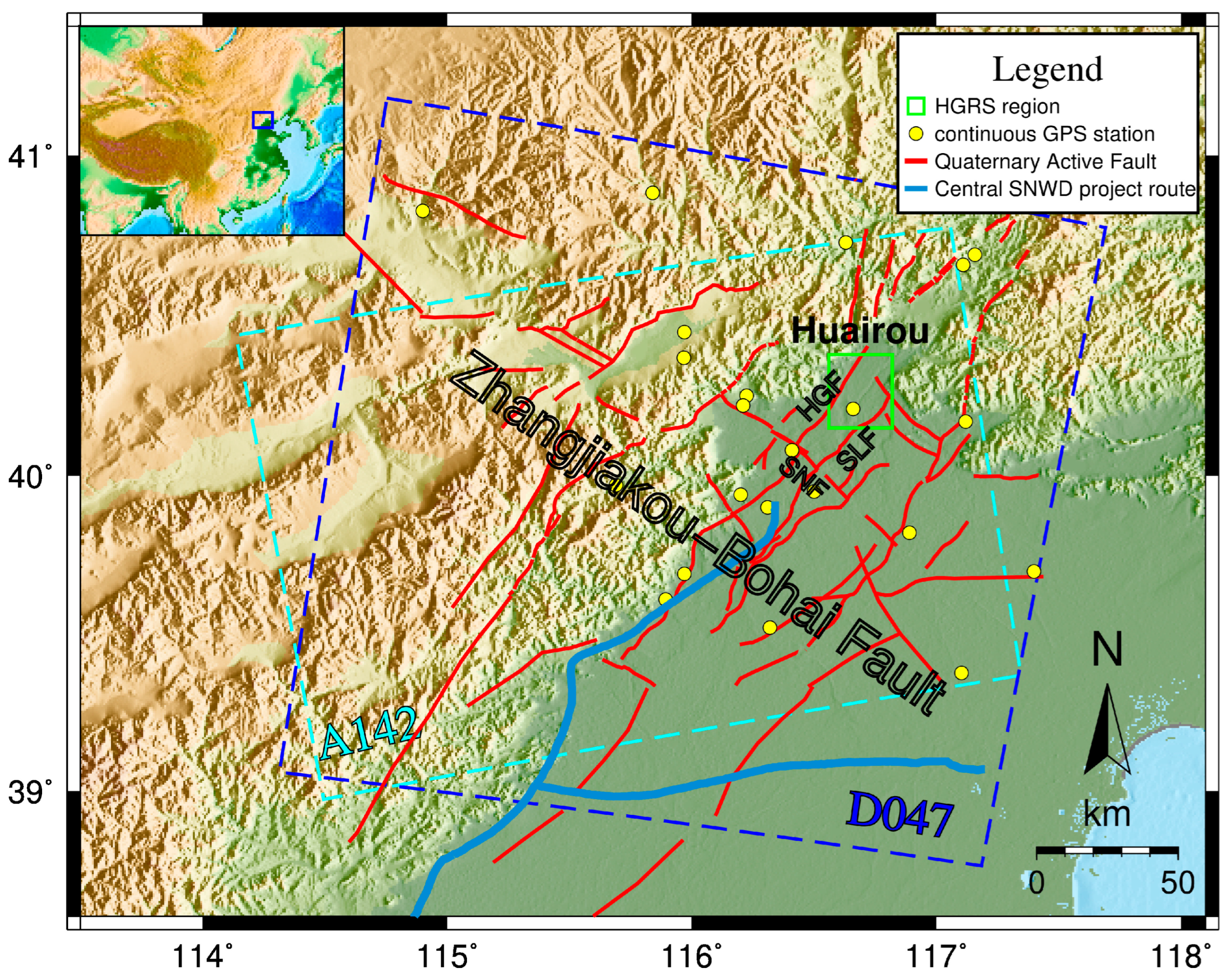
Figure 1.
Tectonic settings of the Beijing area. The dashed boxes show the InSAR data coverage of the study region, cyan for ascending track 142 and dark blue for descending track 47. The red lines mark the quaternary active faults, the northwest trending ones are from the Zhangjiakou-Bohai Fault Zone (ZBFZ), including Sunhe–Nankou fault (SNF), Huangzhuang–Gaoliying fault (HGF), and Shunyi–Liangxiang fault (SLF). The light blue lines show the central route of the South-North Water Diversion (SNWD) Project. Part of the water is transferred through and recharged in the Huairou groundwater reserve site (HGRS) region, which is outlined by the green curve. The yellow circles are the locations of continuous GPS stations in the study region, which are used as a reference in the InSAR data processing.
The South-to-North Water Diversion (SNWD) Project was designed to divert water from the humid south of China to the north to alleviate groundwater shortage in the NCP. This project was launched in 2002 for transporting water from the Yangtze River drainage area through three routes [5]. Since 2015, the Central Route of the SNWD Project has transported water from the Danjiangkou Reservoir on the Han river to more than 20 major cities, including the Beijing (population of 21.9 million) and Tianjin (population of 13.9 million) municipalities and other cities in the NCP [6]. The decline rate of groundwater storage in the NCP slowed down during 2015–2018 [7]. Since 2015, when the SNWD Project started to transport water to Beijing, groundwater exploitation was stopped at the HGRS, and groundwater was recharged gradually, which halted groundwater recession remarkably and even resulted in a water table rise after 2015 [4].
Monitoring water storage is important for water management and estimation of the efficiency of the SNWD Project. Usually, people use water level data to monitor the water storage change [8]. However, sparsely sampled water wells restrict the accuracy of the water storage monitoring. Due to the launch of the Gravity Recovery and Climate Experiment (GRACE) satellites in 2002, monitoring of water storage over a large scale has become available. For example, many researchers have focused on the groundwater storage depletion issue in the NCP using the GRACE satellite observations [9,10]. Because of the relatively low spatial resolution of the GRACE data (300–400 km), this approach cannot resolve the water storage of a smaller region with a <300 km spatial scale well. Space geodetic methods such as InSAR and GPS have been used to monitor hydrologically induced surface deformation, which overcome the spatial restrictions of the above two methods. This method has been applied to many places, such as California [11], Colorado [12], and Utah [13] in the United States, to characterize the aquifer storativity property and monitor the water storage change. Over the NCP, InSAR and GPS studies detected rapid land subsidence caused by groundwater extraction in many cities, including Beijing [14,15], Tianjin [16], Dezhou [17], and Cangzhou [18]. Due to the SNWD Project, water storage has been recovering in recent years, and the HGRS in Beijing has experienced the most dramatic change due to the SNWD Project, providing a unique opportunity to probe into the aquifer storage recovery process in the HGRS region. However, previous studies estimated the groundwater storage change using only sparse groundwater level observation [4,19], and the physical structure of the aquifer system and the groundwater storage response to the SNWD project are still poorly understood.
In this study, we used InSAR and GPS data to detect surface deformation in the Beijing area from 2015 to 2019. We estimated the aquifer storage property in the HGRS region by integrating the uplift deformation and water level change due to the largest recharge of the SNWD Project to the HGRS region at the end of 2018. Finally, we estimated the recharged water storage in the HGRS region at the end of 2018 based on the inverted aquifer storativity. The method developed in this study can also be applied for investigations of groundwater storage change in other regions, such as the entire NCP impacted by the SNWD Project in recent years.
2. Geologic Setting and Hydrological History
Beijing is located on the northwest edge of the NCP. This area generally comprises mountains in the northwest and plains in the southeast. The overlying quaternary strata of the area are composed of alluvial fans and sedimentary depressions [20]. Quaternary unconsolidated sediments are widespread, whose thickness varies from several meters to ~1000 m [21]. The underlying bedrock is cut by several active faults. The Zhangjiakou–Bohai fault zone (ZBFZ) transects the whole Beijing area, composed of several NW-trending left-lateral strike-slip faults, such as the Sunhe–Nankou fault (SNF) [22]. The left-lateral slip rate of the ZBFZ is about 2~3 mm/yr [23,24]. Moreover, several NE-trending faults orthogonally intersect with the ZBFZ, such as the Huangzhuang–Gaoliying fault (HGF) [25] and the Shunyi–Liangxiang fault (SLF) [26], which form several relatively independent sedimentary depressions in the Beijing area. Our study area, the HGRS region (Figure 1), is located in the northeast of Beijing and is one of the alluvial fans traversed by the HGF and SLF from northeast to southwest.
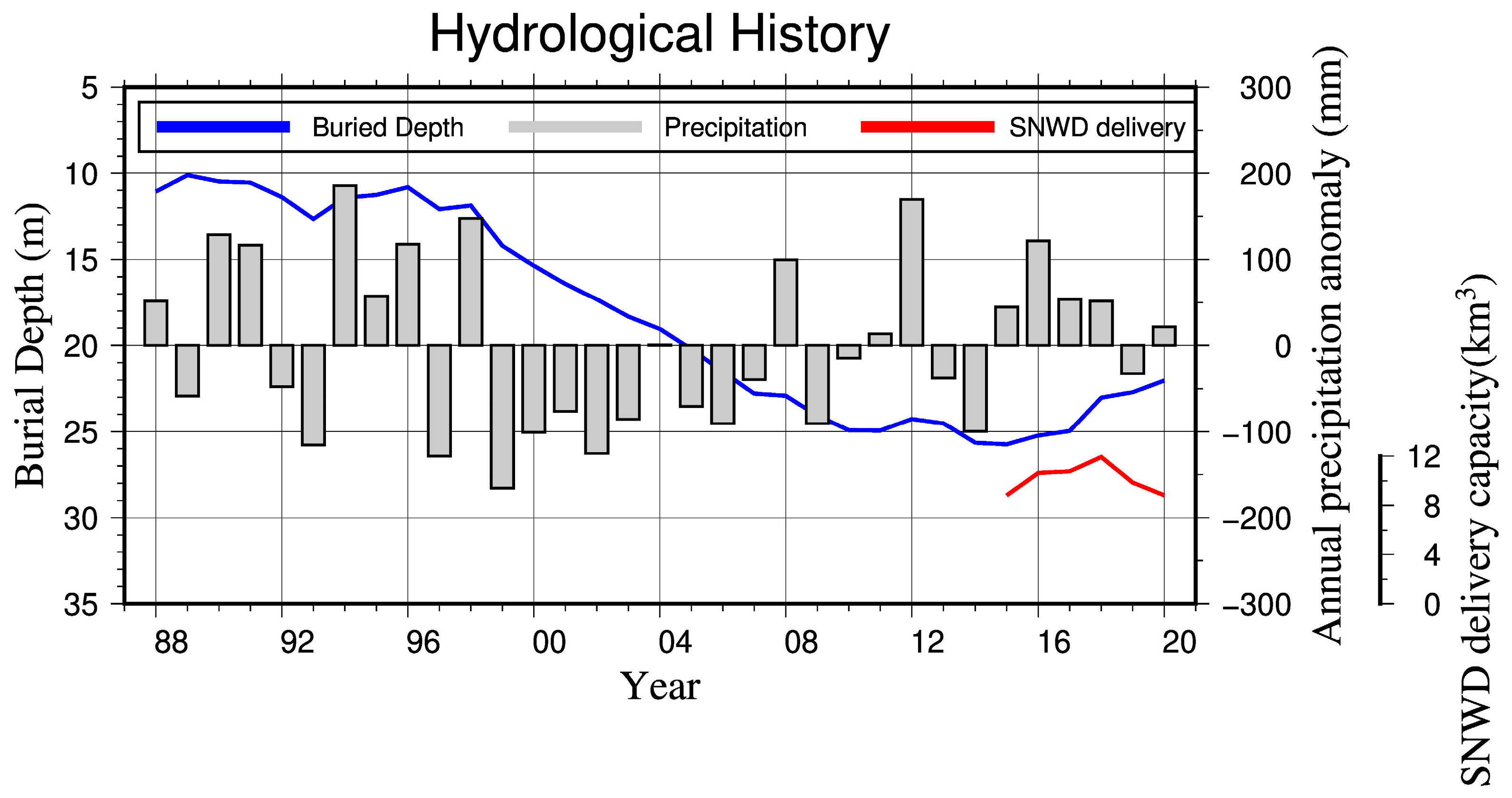
Groundwater storage under the Beijing area has largely been depleted since a prolonged drought during 1999–2007 (Figure 2), which was amplified by increasing anthropogenic water use. The mean precipitation during the same time was only 538 mm/yr, and the fresh water shortage between the water demand and supply was ~1 billion /yr [3]. The consequent groundwater withdrawal led to a long-term groundwater storage decline in the Beijing area. Although precipitation returned to its normal level after 2007, the water level still slowly declined due to metropolitan development and agricultural irrigation. The central route of the SNWD Project started to channel fresh water to the Beijing area from the south in 2015 (Figure 1). About 9.5 billion of water was transported to the Beijing area annually through the Central Route of the SNWD Project [5,6], for public water supply and groundwater recharge. Surrounded by two large-scale reservoirs (the Miyun and Huairou reservoirs), the HGRS region was selected as the major groundwater recharge site for Beijing in September 2015 [4]. The water level in the Beijing area began to recover in 2015 (Figure 2).

Figure 2.
The historical precipitation (grey histogram) and hydraulic burial depth (blue line) records of the Beijing area [3]. The red line shows the water volume delivered to the Beijing area by the SNWD Project each year since 2015.
3. Datasets and Preprocessing
3.1. InSAR Data and Interferograms Generation
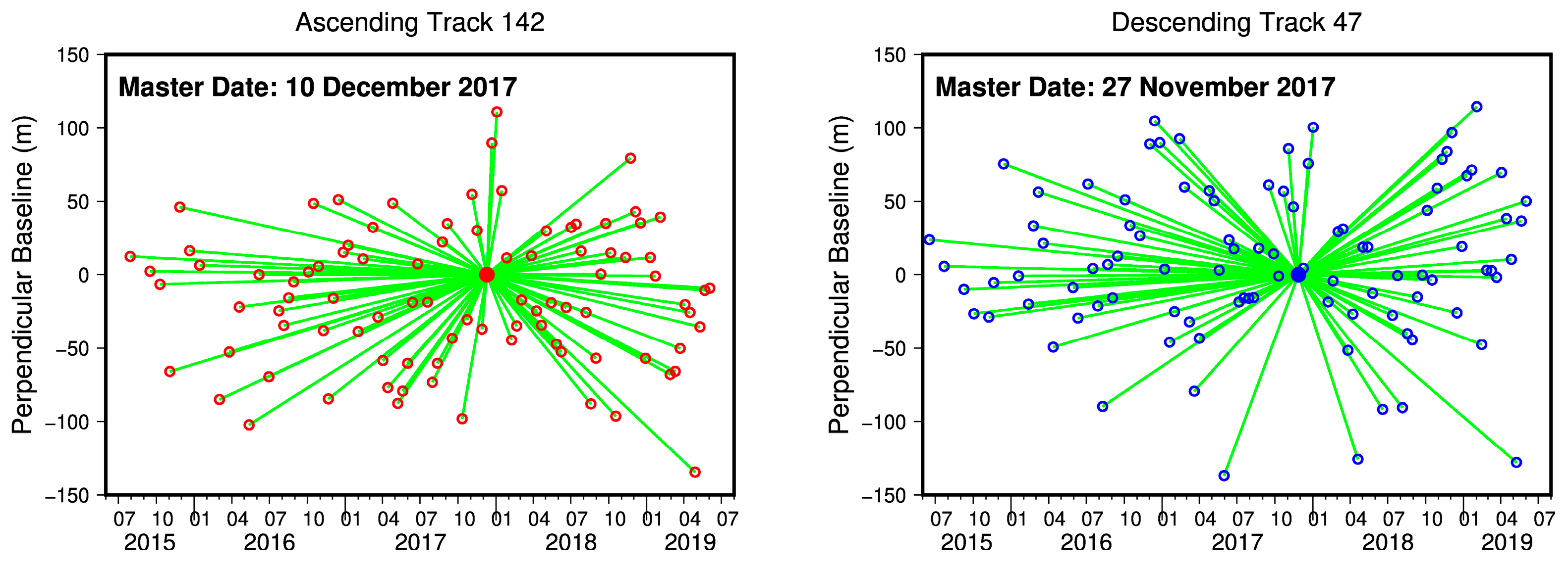
We processed 2 tracks of Synthetic Aperture Radar (SAR) data from the Sentinel-1A/1B satellites recorded between June 2015 and June 2019, including 92 ascending images of track 142 and 96 descending images of track 47 (Table S1). Interferograms were generated using the GAMMA software [27]. The InSAR time series were generated using the Stanford Method for Persistent Scatterer (StaMPS) software package [28]. All of the interferograms were formed with one reference image per track. The selected reference images were 10 December 2017 for the ascending track and 27 November 2017 for the descending track, respectively, to optimize the spatio-temporal coherence (Figure 3).

Figure 3.
The baselines for ascending and descending InSAR tracks. The reference dates are 10 December 2017 (ascending track) and 27 November 2017 (descending track) for optimizing the spatio-temporal baselines. The filled circles denote the reference dates, and the open circles denote the secondary dates.
3.2. GPS Observations
We utilized GPS data observed from both continuous and campaign networks in the NCP, including 36 continuous GPS (CGPS) stations of the Crustal Movement Observation Network of China (CMONOC) observed in 1999–2017 and 25 CGPS stations from the Beijing Continuously Operating Reference Station (CORS) network observed in 2015–2019, of which 22 sites are located in our study area (Figure 1). There are also 437 CMONOC campaign GPS stations located in our study area and observed episodically in 1998–2018. The GAMIT/GLOBK software [29] was used to process the data and produce 3D GPS velocities, which were aligned to the ITRF2014 frame by tying the velocities of globally distributed reference stations. The solution was then transformed into the Eurasia-fixed reference frame using the plate rotation pole [30]. The same reference transformation was performed for the time series data of CGPS stations. We interpolated the spatially discretized campaign GPS velocities to obtain a continuum horizontal velocity field and filter out CGPS outliers using the method of Shen et al. [31].
3.3. Hydraulic Head Data
We collected two sets of well water level data acquired from different sources in the HGRS region. These water wells were from both unconfined and confined aquifers (Figure 4). Three stations prefixed with “GD” were from the National Earth System Science Data Center, National Science and Technology Infrastructure of China, and the data were collected 2005–2018 with 1-month sampling interval. All of these wells were attached to the confined aquifer. Twelve stations prefixed with “MC” were from the National Groundwater Monitoring Center of China, and the data were collected from January 2018 to December 2019 with a 5-day sampling interval. Five of these sites had wells attached to both unconfined and confined aquifers while the rest of them only had wells attached to the confined aquifer. Observation errors in the digital pressure sensors used for most wells in the well water level observation network of China were no more than 10 mm [32].
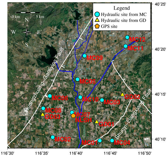
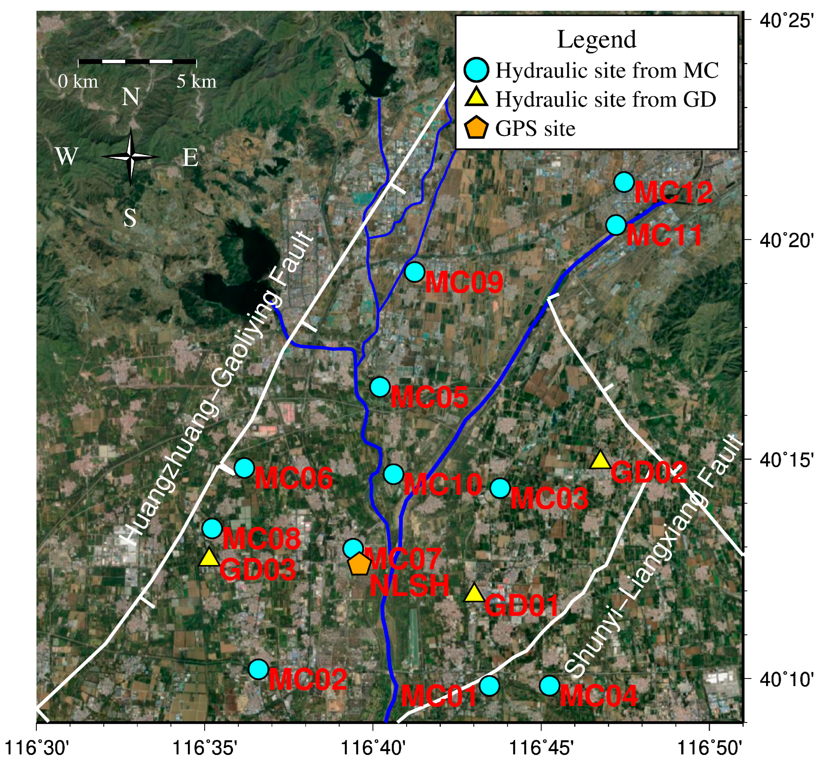
Figure 4.
Optical image of the HGRS region. The fault traces are marked as white lines, including the HGF and the SLF. The major rivers are marked as blue lines. Cyan circles are hydraulic monitoring sites from the National Groundwater Monitoring Center of China, and yellow triangles are hydraulic monitoring sites from the National Earth System Science Data Center, National Science and Technology Infrastructure of China (http://www.geodata.cn, last accessed on 15 April 2021). The orange polygon is the continuous GPS station NLSH, chosen as the reference station.
The water level raised significantly from 6 October 2018 to 22 January 2019 due to the groundwater recharge by the SNWD Project, and the process was recorded well by both the well water level and the InSAR data. We, therefore, used the water level and surface uplift data observed during the same time period to estimate the aquifer’s storativity.
4. Methods
4.1. InSAR Time-Series Data Analysis and Atmospheric Noise Correction
The decorrelation effects of radar signals are the major issues in InSAR application, especially in the luxuriant area. As the main grain production base, the vegetation in the NCP makes it difficult to recover deformation signals of long time intervals using the traditional InSAR data processing method. However, when SAR pixels are dominated by few point targets, the decorrelation effects can be greatly reduced. These targets are called persistent scatterers (PSs) [33]. We used the StaMPS software [28] to generate the PS time series. StaMPS identifies PSs based not only on the amplitude characteristics but also on the phase stability [34], which can identify densified PS targets in all terrains and overcome the decorrelation problem in vegetated mountainous areas without man-made constructions. Finally, we identified ~ PS in our study area. We used parallel computing algorithms to deal with the high computing demand by dividing the study area into overlapping patches. The topographical phase effects were removed using a digital elevation model (DEM) from the Shuttle Radar Topography Mission (SRTM) with approximately a 30-m resolution [35].
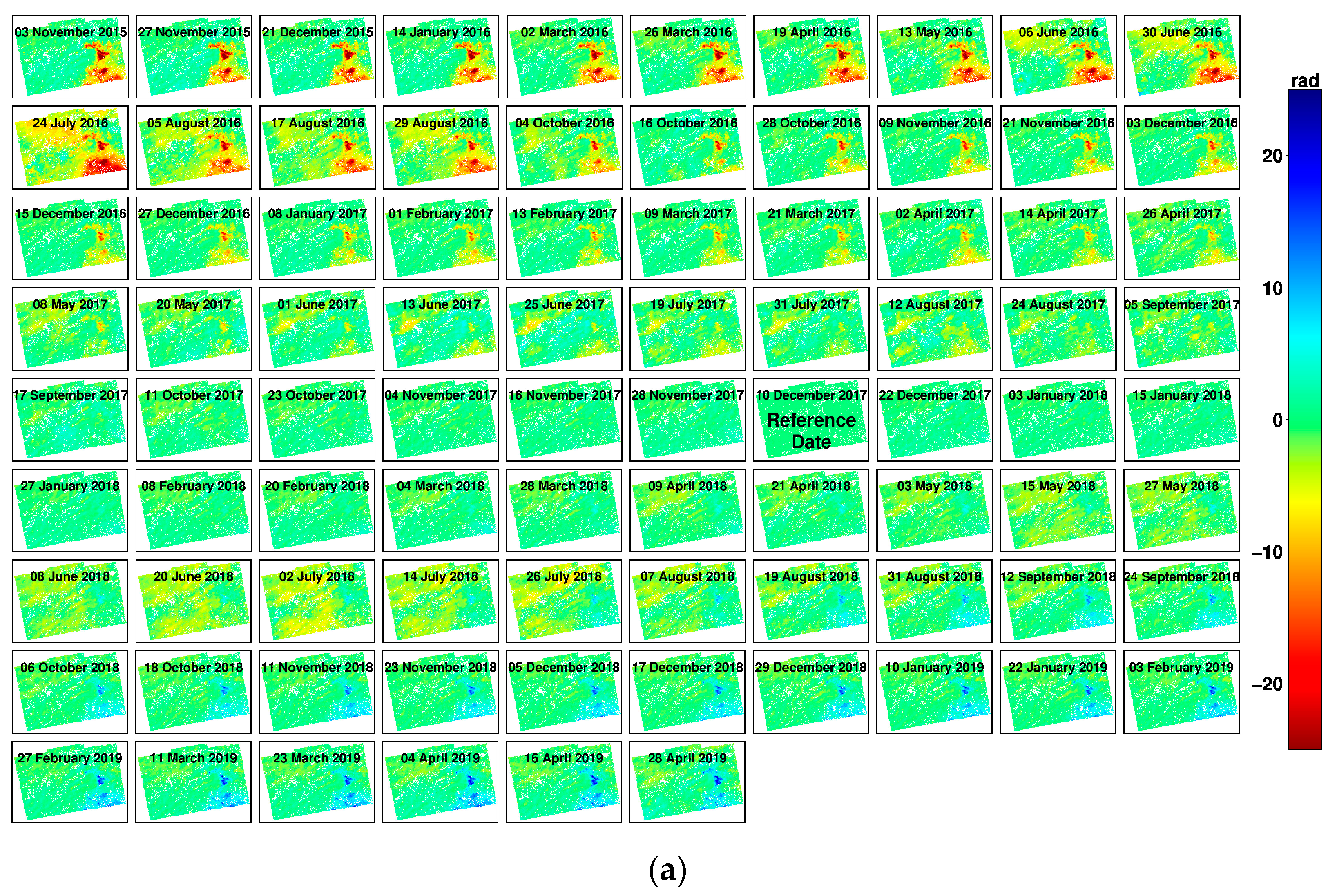
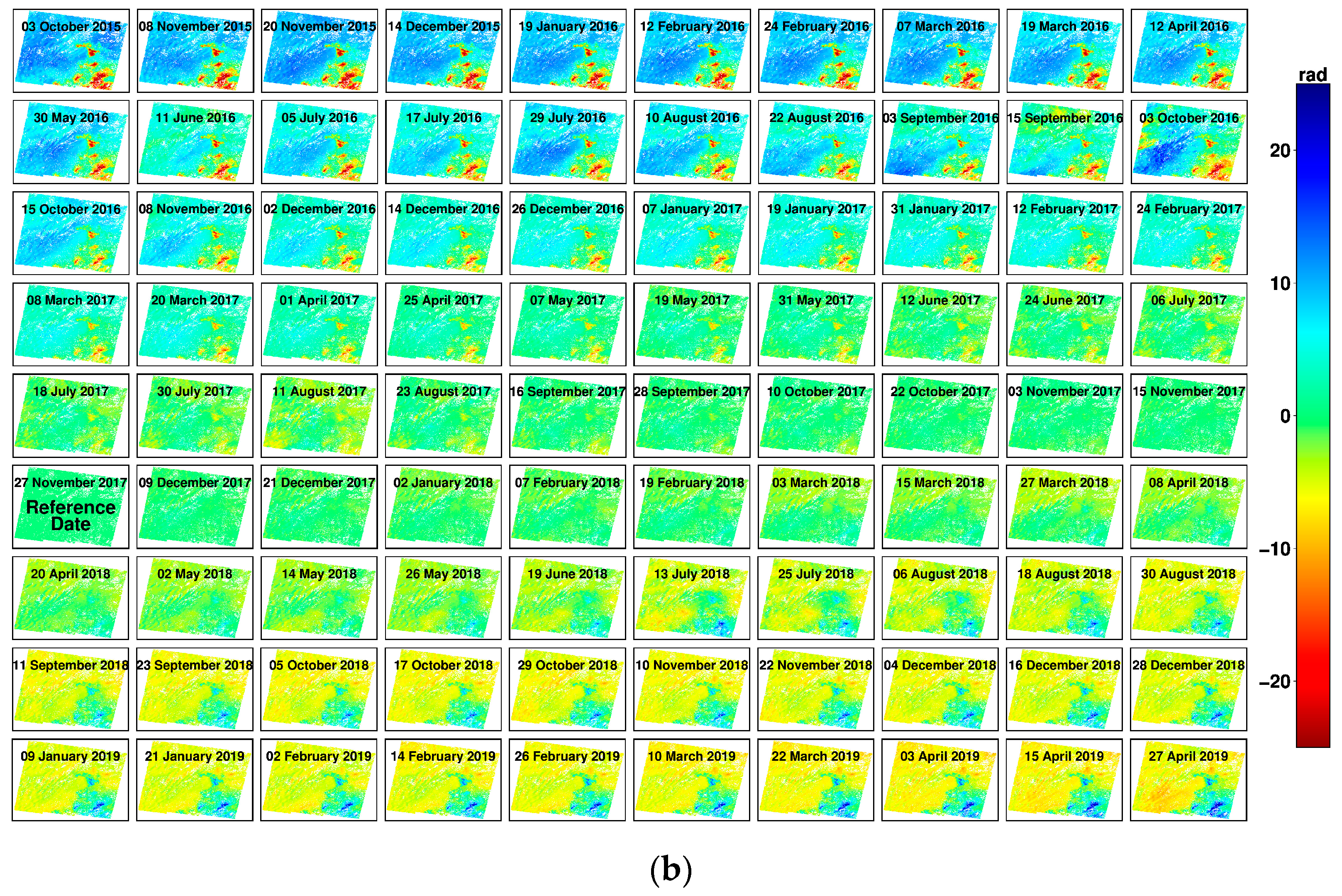
A main challenge in InSAR application is the reduction of atmospheric noise disturbance. We used two methods to estimate and reduce the atmospheric phase screen (APS). First, we used the atmosphere model ERA5 [36] to estimate the APS. Released by the European Centre for Medium-Range Weather Forecasts (ECMWF), ERA5 provides hourly estimates of a large number of atmospheric variables. The data cover the ground on a 31-km grid and resolve the atmospheric change with 137 pressure levels in the vertical direction up to a height of 80 km. We used the Matlab software package Toolbox for Reducing Atmospheric InSAR Noise (TRAIN) [37] to estimate the APS model. However, this correction was not sufficient to remove the local spatio-temporal changes of the atmospheric content. Then, we used the Common Scene Stacking (CSS) method [38,39] to suppress the residual APS and stochastic noise. The first and last three images were removed from the InSAR time series due to their shortage of observation epochs. The unwrapped phase time series data for ascending track 142 and descending track 47 after atmospheric correction are shown in Figure 5a,b, respectively. The unwrapped phase time series for the two tracks without atmospheric correction are provided in the Supplementary Materials. In this way, we removed 77.4% and 53.9% of the APS for the 2 tracks, especially in the luxuriant summer season.
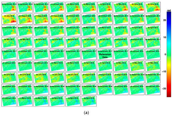
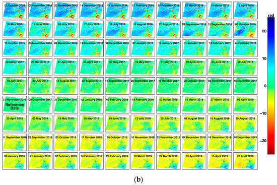
Figure 5.
(a) Unwrapped phase time series for ascending track 142 after atmospheric correction. (b) Unwrapped phase time series for descending track 47 after atmospheric correction.
4.2. Synthesis of InSAR and GPS Time Series Data
InSAR and GPS are two widely used satellite geodetic methods in crustal deformation monitoring. The GPS can precisely measure three-dimensional displacement at a discrete location, with up to one-millimeter accuracy in the horizontal direction and several-millimeter accuracy in the vertical direction [40]. The conventional InSAR technique can measure one-dimensional deformation in the radar line-of-sight (LOS) direction with large spatial coverage, with up to several millimeters to centimeter accuracy [41]. The synthesis of InSAR and GPS measurements can acquire better spatial and temporal resolution than using either one of them. Compared with InSAR, CGPS observations are less prone to signal disturbances, and can be treated as the ground truth. We projected the GPS data to the InSAR LOS direction and computed the differences between the InSAR and CGPS observations to correct the orbital and other long-wavelength errors of the InSAR data. For each InSAR interferogram, LOS differences were evaluated at multiple GPS sites and were used to estimate the orbital correction using the least-squares algorithm. The correction can be the offset only or offset plus 1-D or 2-D linear trend, depending on the signal feature in the study area. In this study, we used 17 CGPS sites in the ascending track 142 and 18 CGPS sites in the descending track 47 to estimate the constant offsets for both tracks to avoid overfitting of the phase trend. The time series comparisons between the InSAR and CGPS data are shown in Figure 6a,b for the two tracks, respectively, showing that the scattering of the InSAR time series was suppressed significantly after the offset correction.
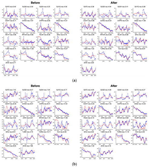
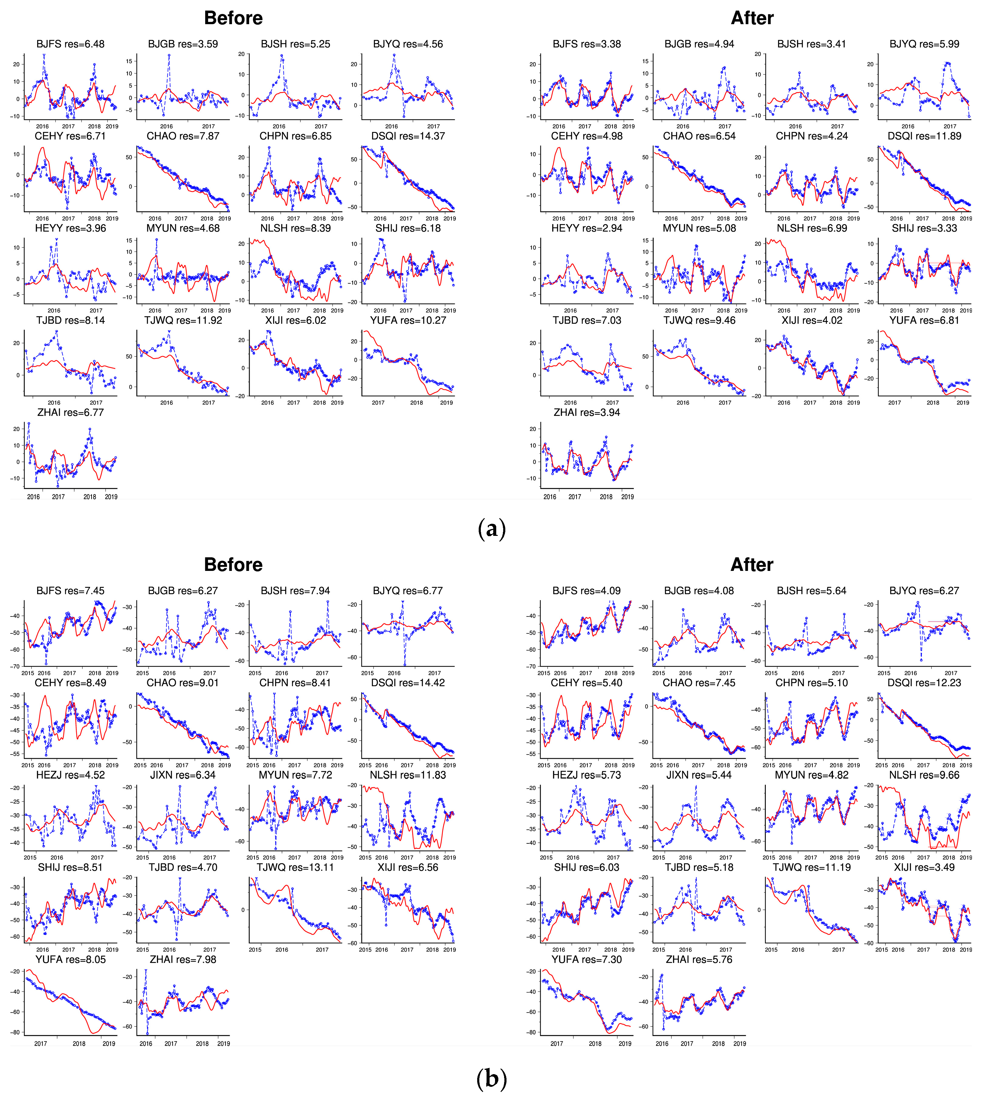
Figure 6.
(a) Time series comparison at continuous GPS stations in ascending track 142. Blue points are InSAR time series and red lines are GPS time series, which are projected in the LOS direction. The left and right panels are the results before and after offset correction, respectively. (b) The same as Figure 6a but for the descending track 47.
Using the corrected InSAR time series data, we derived the mean LOS velocity field through least squares regression. In this case, the InSAR time series data were transformed to the Eurasia-fixed reference frame defined by the GPS data (Figure 7a,b). An assumption was needed to recover a 3D velocity field using the InSAR data of two LOS directions. The tectonic deformation field in the Beijing area is primarily horizontal and dominated by left-lateral shear across the SE-trending ZBFZ [42]. Therefore, we assumed that the NE-oriented horizontal velocity is negligible and used two tracks of the corrected mean LOS velocity and corresponding time series to invert for the vertical and SE-oriented mean horizontal velocity and corresponding time series (Figure 7c,d).
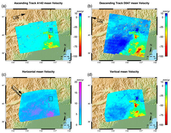
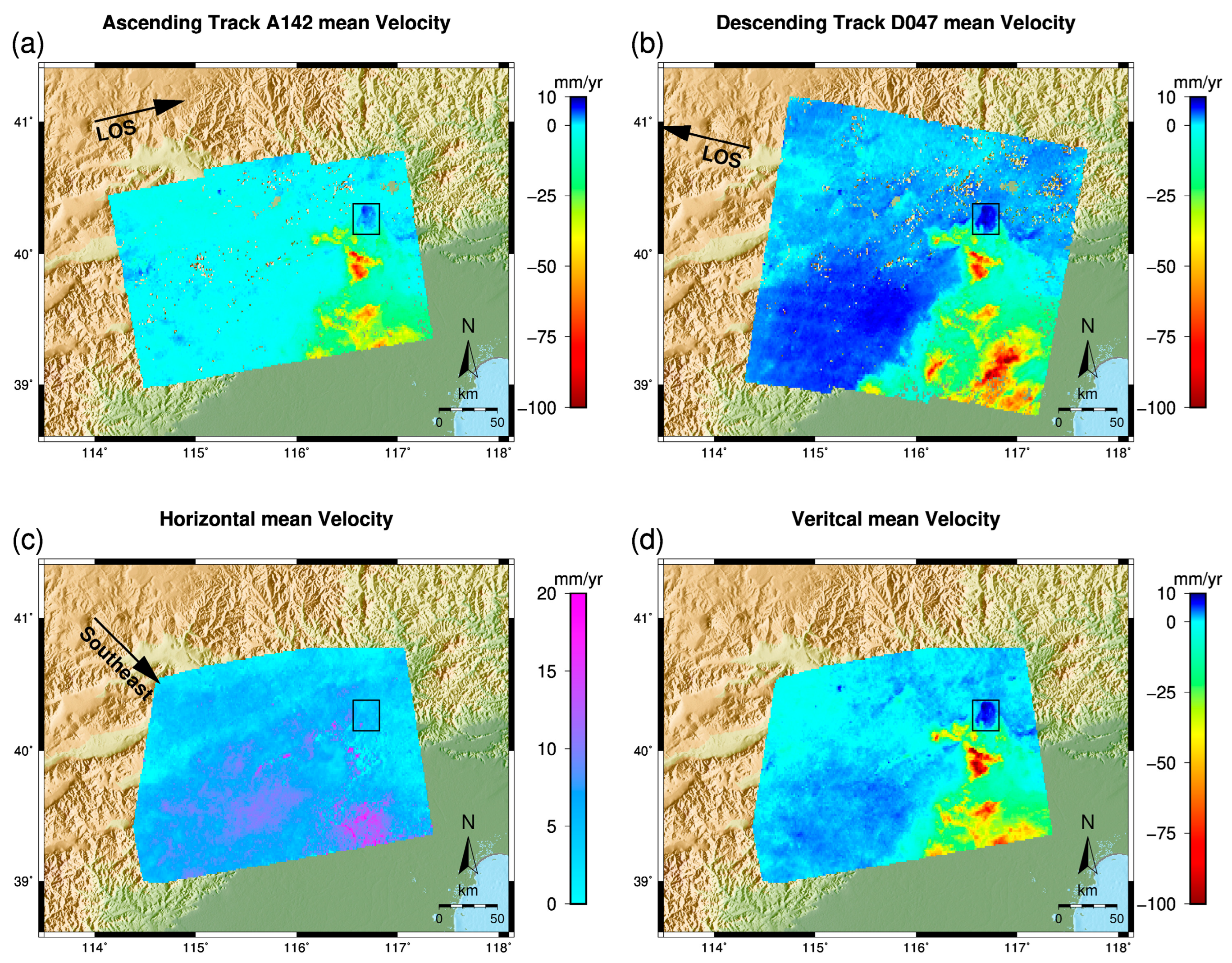
Figure 7.
InSAR data results. (a,b) InSAR A142 and D047 mean LOS velocities. (c,d) Horizontal and vertical mean velocities resolved by considering only the southeastern and vertical components of the displacement field. Black rectangle marks the HGRS region.
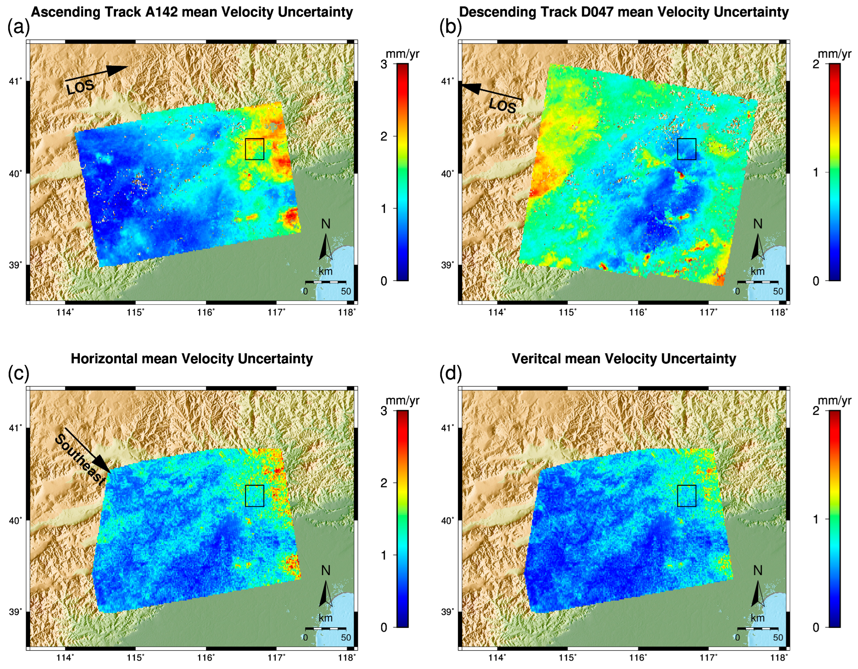
We used the bootstrap method to estimate the uncertainties of the mean LOS velocities [28], which were propagated to the uncertainties of the horizontal and vertical mean velocities. Details of the derivation are provided in the Supplementary Materials. The uncertainties of the surface deformation resolved by InSAR are shown in Figure 8, which shows that the uncertainties of the horizontal and vertical mean velocities were no more than 3 and 2 mm/yr, and particularly < 1 mm/yr for both components for the HGRS area.
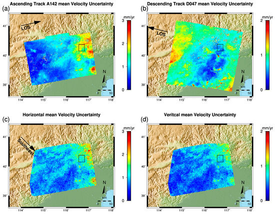
Figure 8.
Uncertainties of the InSAR data results. (a,b) Uncertainties of the InSAR A142 and D047 mean LOS velocities. (c,d) Uncertainties of the horizontal and vertical mean velocities. Black rectangle marks the HGRS region.
4.3. Aquifer Storage Properties Estimation
Aquifer storage properties are important hydrological parameters for groundwater assessment and management. The storativity is defined as the volume of water released from the total porous medium per unit decline in hydraulic head, per unit area [43]. It can be written as:
where is the specific storage [1/m] and is the thickness of the aquifer [m]. The specific storage can be expressed as , where is the density of water [kg/m3], is the gravity acceleration 9.8 m2/s, is the compressibility of the aquifer [1/Pa], is the porosity, and is the compressibility of the water [1/Pa]. Because the compressibility of an aquifer is two orders of magnitude larger than the compressibility of water [43], we can ignore the water volume change due to the water expansion, and yield:
In a laterally extended aquifer, the deformation of the aquifer only occurs in the vertical direction; then, the compressibility of an aquifer can be expressed as:
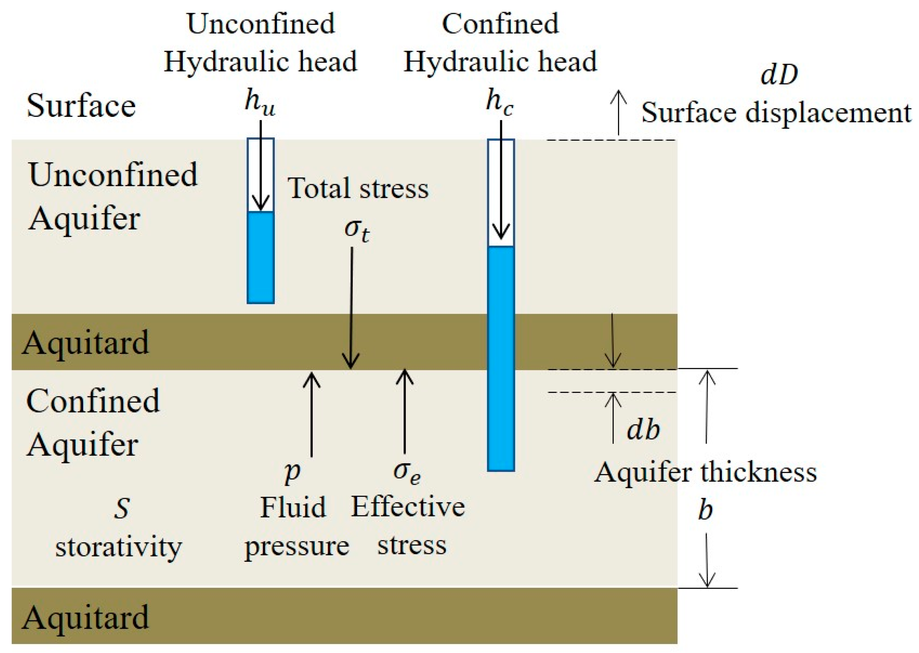
where is the change in the aquifer thickness due to the change in the effective stress , and positive means uplift (Figure 9). Accordingly, the aquifer’s storativity can be written as:
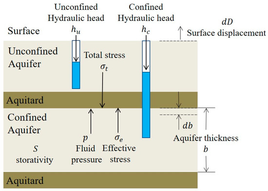
Figure 9.
A conceptual model of the aquifer deformation system. The aquifer system consists of permeable aquifers and relatively impermeable aquitards. Wells at different depths can monitor hydraulic head changes in the shallow unconfined aquifer and deep confined aquifer.
The change in the aquifer thickness can be observed by InSAR or GPS, and the change in the effective stress can be measured from water levels. Therefore, the integration of surface deformation and water level data can constrain the aquifer storage property. The storativity used here is related to elastic deformation only; therefore, it is often called elastic skeletal storativity.
Based on the principle of effective stress [44], the extraction of water can reduce the pore pressure and increase the effective stress to induce land subsidence, causing both elastic (recoverable) and inelastic (permanent) compaction. The elastic compaction can occur in both sand and clay layers (aquifers and aquitards) while the inelastic deformation occurs only at the aquitard layers, which cannot be recovered. If there is a groundwater recharge to the aquifer system, it can induce land uplift due to the recovery of the elastic part of the aquifer system. Therefore, we used the most significant uplift surface deformation and the related increase in water levels in HGRS due to the recharge of SNWD project at the end of 2018 to resolve the elastic skeletal storativity of the aquifer.
Since the pore pressure change in the HGRS region is due to the surface recharge, the hydraulic condition in the unconfined aquifer is changed, which might affect how we estimate the aquifer storativity. We, therefore, estimated the aquifer storativity under three different situations. For the first situation, the change in the effective stress is only due to the pore pressure change in the confined aquifer and the surface deformation is only due to the elastic rebound of the recharged confined aquifer. As the effective stress , where is the total loading stress and is the pore pressure, the total loading stress is unchanged, and the change in the effective stress is . Accordingly, the storativity is:
where is the water level change observed in the confined aquifer, and positive means a water level increase. The change in the aquifer thickness equals the surface deformation observed by InSAR. For the second situation, we considered the effect of the water storage change in the unconfined aquifer on the change in the effective stress. The recharge in the unconfined aquifer would increase the total loading stress by , where is the porosity of the unconfined aquifer and is the water level in the unconfined aquifer. Therefore, the change in the effective stress is ). Accordingly, the storativity is:
The change in the aquifer thickness also equals the surface deformation observed by InSAR. For the third situation, we considered the subsidence and caused by the mass loading of the water in the unconfined and confined aquifers, respectively. The deformation due to the mass loading can be theoretically calculated using a rectangular loading in a homogeneous elastic half-space [45]. Therefore, the deformation due to the elastic rebound of the confined aquifer is . Accordingly, the corresponding storativity is:
For the first situation, using InSAR-derived vertical surface deformation and confined water level change data , we can estimate the storativity by employing Equation (5). Moreover, using unconfined water level change data , we can estimate the storativity by employing Equation (6) at specific locations. To eliminate the deformation caused by mass loading of the recharged surface water, it needs to estimate the mass loading of the surface water first. The water storage in the confined aquifer can be obtained using the storativity over the whole area. This would make the evaluation of nonlinear. Using a given porosity and initial storativity , we can determine the mass loading-induced deformation and first. Second, using an initial confined water level change , we can obtain the value of by employing Equation (7). Then, we update the and values to reestimate the new values of and through Equation (7). We performed this derivation iteratively until the results converged.
5. Results and Analysis
5.1. Surface Deformation in Beijing Area
Following the method described in Section 4.2, we integrated the GPS and InSAR data to derive the mean horizontal and vertical velocities in the Beijing area during 2015–2019 respectively (Figure 7c,d). The mean horizontal velocity field is in general consistent with the tectonic deformation and the horizontal GPS velocity results (Figure S3). However, when decomposing the LOS observations into the horizontal and vertical displacements, the errors of the two components are correlated, and the error of one component is associated with the error of the other component. Due to severe land subsidence in Beijing area, the error of vertical displacement is large due to its nonlinear behavior, and the horizontal deformation estimation is thus contaminated by the correlated error with the vertical velocity component, making it hard to precisely determine the horizontal velocity field from the LOS data, and the subtle velocity gradient across the ZBFZ [42] is, therefore, not clearly visible in Figure 7c.
The surface deformation in the Beijing area is dominated by vertical motion. In Figure 7d, we can see remarkable subsidence occurred in the southeastern plain area, up to 100 mm/yr, which is the most populated and intensive agricultural area. However, in the northeast, the HGRS region shows a dramatic uplift motion at a rate of ~10 mm/yr (black rectangle in Figure 7d). In the southwest mountainous area, there is also a widely distributed minor uplift at about 2~3 mm/yr. In this study, we focused on the uplift deformation in the HGRS region caused by the recharge of the SNWD Project (Figure 10a), which is remarkable in contrast to the surrounding regions with subsidence or minor uplift.
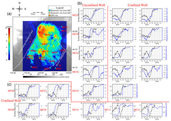
Figure 10.
Hydraulic and InSAR spatial and temporal observations. (a) InSAR-determined mean vertical velocity field of the HGRS region in 2015–2019 overlying the regional digital elevation map. The fault traces are marked as white lines, including the HGF and the SLF, which roughly bound the uplift area. Cyan circles and yellow triangles are hydraulic monitoring sites, and the orange polygon is the continuous GPS station NLSH. (b) Confined and unconfined hydraulic head observations at five wells. Blue lines are the hydraulic head and black lines are surface vertical displacements, respectively. (c) Confined observations at other seven wells.
5.2. Aquifer’s Storativity Property
We first used the well water head and surface displacement data to determine the storativity following Equation (5) for the confined aquifer without considering the water storage change in the unconfined aquifer. To do so, we selected the data from the National Groundwater Monitoring Center of China. These data were recorded automatically at a high sampling rate (5-day) and are of higher quality compared to the data from the National Earth System Science Data Center, whose 1-month sampling interval is too large for the data to be effectively used for model constraint (Figure 11a). Ten wells in the interior of the HGRS, MC01 to MC10, were chosen, and the wells MC11 and MC12 were excluded because they are located at the edge of the HGRS, whose aquifer settings may be different from the rest of the sites (Figure 10a). We, therefore, chose a segment of the data spanning 6 October 2018 to 22 January 2019, during which both the water head and surface displacements showed a remarkable proportional increase (Figure 10b,c and Figure 12).
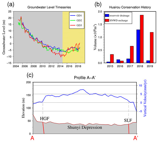
Figure 11.
Synthetic analysis of geodetic and hydraulic data. (a) The long-term groundwater level observation time series in the HGRS region at sites GD01, GD02, and GD03 from year 2005 to 2018. (b) The water conservation history of the HGRS region from Li et al. [4]. Blue and red bars are for the reservoir drainage and recharge water volumes from SNWD each year, respectively. (c) The InSAR-determined vertical velocity and elevation along the A-A’ profile shown in Figure 10. The Shunyi Depression is produced by normal faulting of the HGF and SLF.
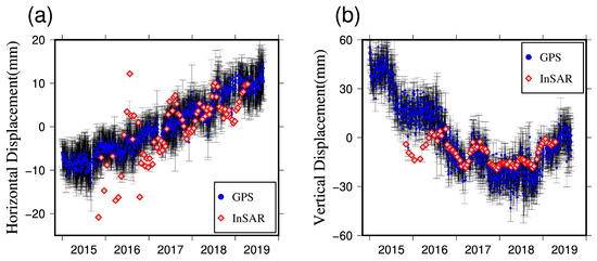
Figure 12.
The time series of the reference GPS station NLSH in the HGRS region (blue dots), compared with the InSAR-determined horizontal (a) and vertical (b) surface displacements (red dots), respectively.
Following Equation (5), we derived the values at the 10 wells using the water head and surface vertical displacement data. The determined values range from to (Table S2). We then performed a spatial interpolation of the values using the bounded linear kriging algorithm [46] and compared it with the thickness contour of the quaternary sedimentary [21] (Figure 13). A strong correlation exists between the spatial distribution of storativity and the sedimentary thickness, indicating the region with a thicker layer has larger storativity, and vice versa.
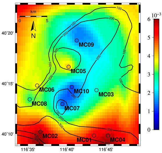
Figure 13.
The spatial distribution of storativity in the HGRS region, interpolated using data at sites marked by circles. The black contours show the thickness of the quaternary sedimentary layer [21].
To consider the contribution of water storage change in the unconfined aquifer to the effective stress change, we followed Equation (6), again not considering the vertical deformation caused by the mass loading effect, to estimate the storativity . To do so, the observed water level data in the unconfined aquifer are essential. Five sites in the HGRS region have water level observations from wells in both confined and unconfined aquifers (MC01-MC05). The porosity of the unconfined aquifer is 0.21, which is based on the hydraulic study of the sediment layer of the NCP [47]. The corresponding storativity values range from to at the five sites (Table S2).
A further improvement of the estimation of storativity is to take into account deformation due to mass loading of the water storage change in both the unconfined and confined aquifers, corresponding to the terms and in Equation (7). The calculation of mass loading was performed assuming the deformation of an elastic continuum, with water storage change in the unconfined and confined aquifers as the loading source, and the porosity of the unconfined layer [47]. The mass loading in the unconfined aquifer is , where is the surface area of the aquifer within our study area, and is the spatial distribution of the water level change for the unconfined aquifer interpolated from the well observations. The mass loading in the confined aquifer is , and were interpolated from the confined aquifer results. The deformation caused by mass loading of the recharged water is , calculated using a rectangular load in a homogeneous elastic half-space [45]. Since also appears in the confined aquifer loading calculation, the estimation of needs to be carried out iteratively. Using the surface vertical deformation derived from InSAR data (Figure 14), the initial value of storativity is taken as and the initial value of the pore pressure change in the confined is taken as , which were used to derive , and was determined using Equation (7). Then, the updated and were used to calculate , and the computation was iterated until the solution converged. The final estimates of storativity range from to (Table S2). The unconfined water level change was estimated by carrying out kriging interpolation of unconfined water level observations (MC01-MC05) and a priori information about tectonic settings (Figure 15a). The confined water level change was predicted with the estimation of (Figure 15b). The estimation of is shown in Figure 16, which also indicates that the spatial distribution of storativity correlates well overall with the thickness of the quaternary sedimentary layer.
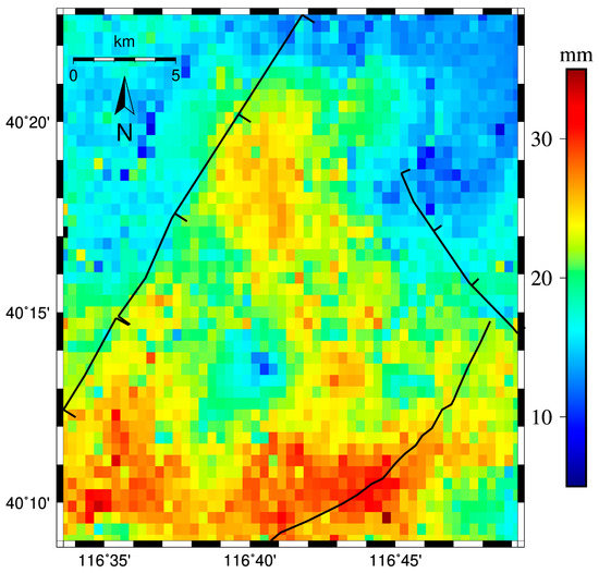
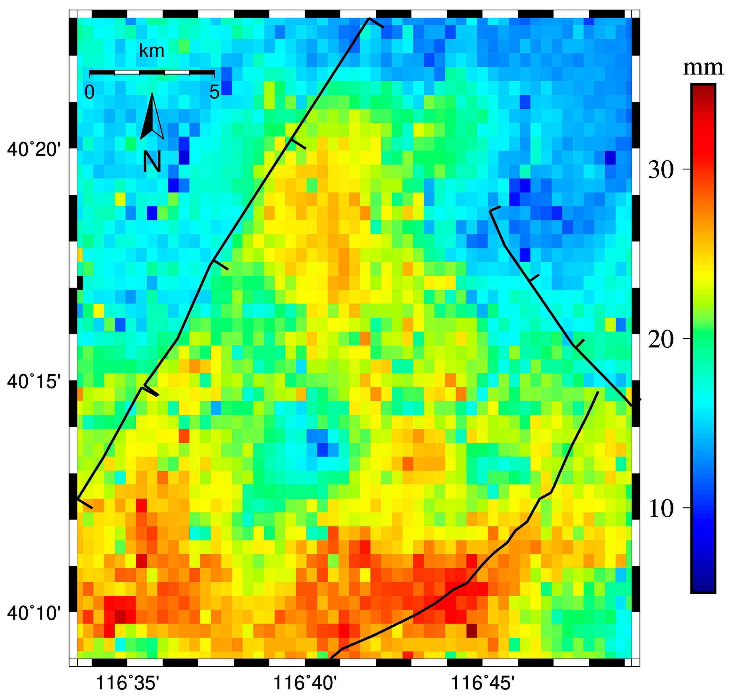
Figure 14.
The surface vertical deformation derived from InSAR data observed from 6 October 2018 to 22 January 2019; black lines mark the faults.
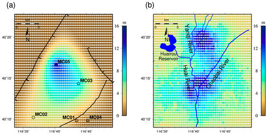
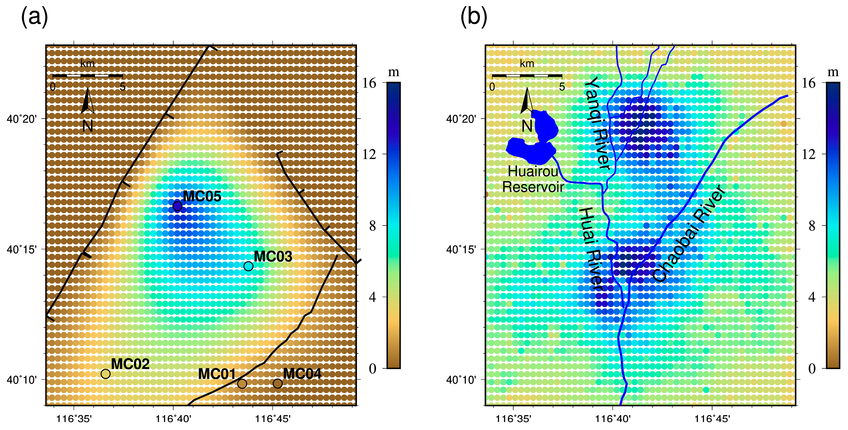
Figure 15.
Estimation of the water level changes for (a) the unconfined aquifer and (b) confined aquifer from 6 October 2018 to 22 January 2019 based on the storativity ; black lines mark the faults and blue lines mark the major rivers and the Huairou reservoir.

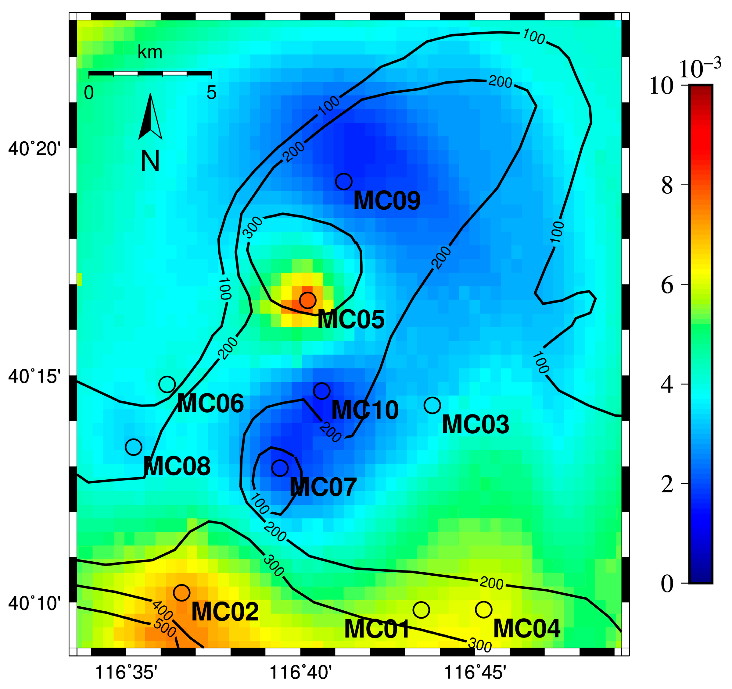
Figure 16.
The spatial distribution of storativity in the HGRS region. The black contours show the thickness of the quaternary sedimentary layer [21].
Based on Equations (5)–(7), the uncertainties of storativity estimates were calculated using the formulas:
where is the uncertainty of the surface vertical velocity, and and are the uncertainties of the confined and unconfined well water level. Since the uncertainties of the water level are small, the uncertainties of the storativity estimates , , and are all dominated by , and are no more than . The storativity uncertainties of all the wells are listed in Table S2. It should be pointed out that all the storativity uncertainties we have dealt with so far are formal uncertainties of specific wells, which were derived under the assumption of 1-d media structure. The actual uncertainties should be greater than that, given that the 3D variation of the media will introduce additional error. This error, however, is difficult to quantify because of the limited sub-surface information we have. Even though, the general layered sediment structure of the HGRS ensures that the errors are much smaller than the storativity estimates. Additionally, because the three storativity estimates share the common error source related with the media, their relative values should be less prone to the error and more reliable.
5.3. Estimation of Recharged Groundwater in the HGRS Region
The recharged water storage in the confined aquifer can be estimated by integration of the storativity times the water level change over the area of the confined aquifer (Figure 15b). According to the estimated aquifer storativity and shown in the previous sections, the corresponding recharged water volume from 6 October 2018 to 22 January 2019 in the confined aquifer is .
The recharged water storage in the unconfined aquifer can be estimated by integration of the change in the water level times the porosity over the surface area of the unconfined aquifer. The corresponding recharged water from 6 October 2018 to 22 January 2019 in the unconfined aquifer is then ~. However, due to the lack of sufficient well data in the unconfined aquifer, this result is preliminary.
The water conservation data shows that of water was drained from the Miyun and Huairou reservoirs and of water was recharged from the SNWD Project in 2018 [4] (Figure 11b), and most of the recharges and drainages occurred in the second half of 2018 [48]. Comparing the total water recharged at the surface and the water storage change in the confined and unconfined aquifers, we see that about 4% of the surface water was successfully recharged into the confined aquifer and about 91% into the unconfined aquifer, respectively, which is consistent with the estimation using hydrological observations only [48].
5.4. Characterizing Fault Locations from Hydraulic-Related Deformation
Lots of studies have shown that faulting activities may cut the water aquifer layers and fill the faults with clays, making the hydraulic conductivity of the faults several orders of magnitude lower than the surrounding aquifer system and blocking fluid flow across the fault [11]. As shown in Figure 10a, the normal faulting of the HGF and SLF in the HGRS region roughly bounds the uplift area and constrains the groundwater recharge in the Shunyi Depression. We can see the abrupt change in the hydraulic-related vertical velocity across the two faults along the profile A-A’ in Figure 11c. Hydraulic-related deformation may be a useful way to pin down the locations of blind active faults.
6. Discussion
6.1. Uncertainty of Aquifer Storativity Estimation
Considering that the storativity is linearly dependent on the aquifer thickness , it is predictable that storativity has a good spatial correlation with the quaternary sedimentary layer thickness, which provides an independent verification for the spatial distribution of storativity. Moreover, the storativity values in the NCP alluvial plain aquifers range from to according to hydrological studies [49], which are consistent with our results.
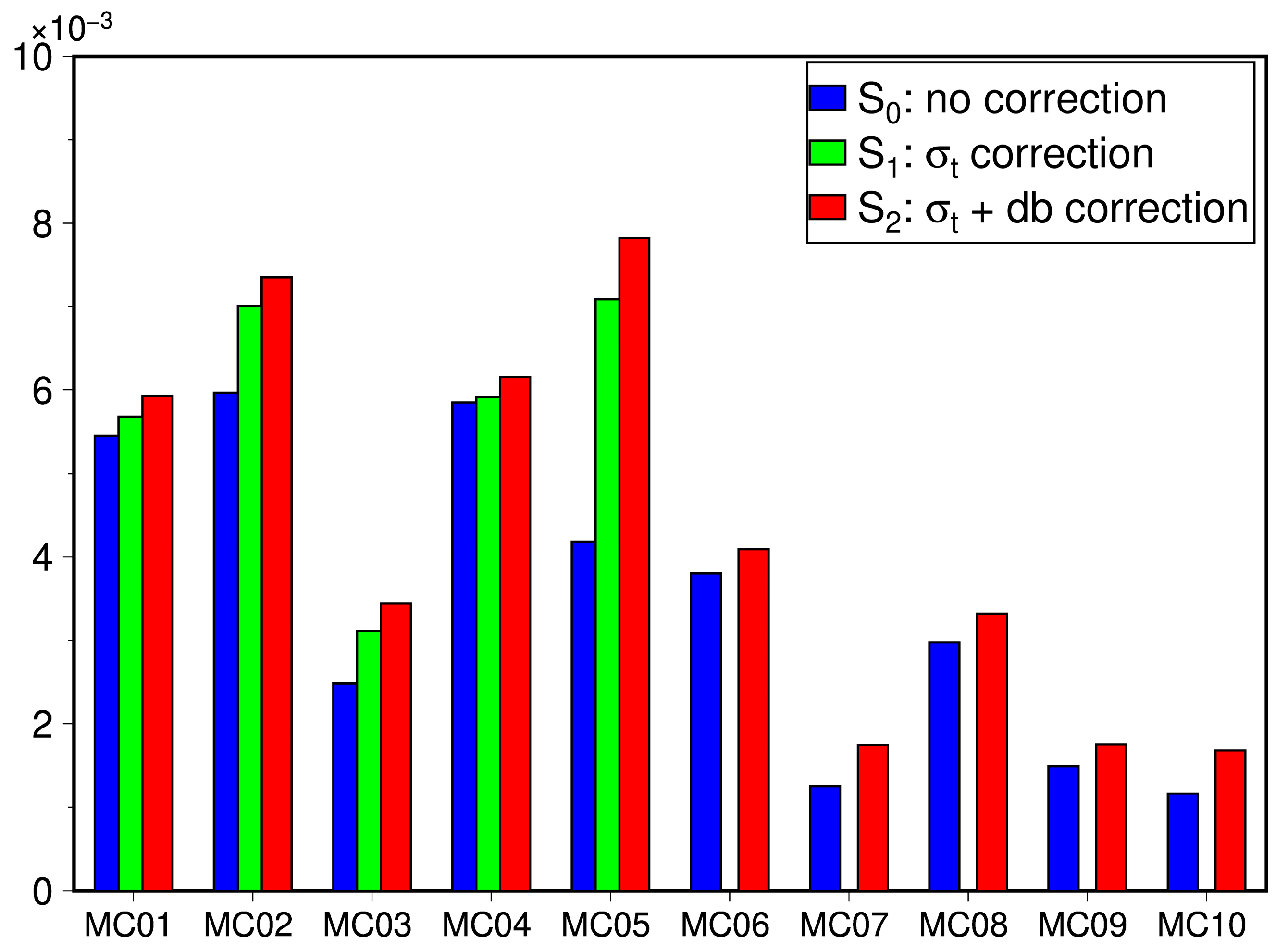
Comparing the aquifer storativity estimates under three situations, we can estimate the influence of the recharged water in the unconfined aquifer quantitively. The storativity estimates in the three situations for wells MC01 to MC10 are shown in Figure 17. The corrections for different wells vary significantly, which are almost negligible for well MC04 but almost as large as the original for well MC05. On average, there is a 23% increase from storativity to and a 28% increase from and but only a 7% increase from and . This result shows that the contribution of the water storage change in the unconfined aquifer to the effective stress is not negligible; however, the deformation due to the mass loading of the recharged water is a small contribution to the surface deformation. By comparison of the estimated storativity for all the situations, the estimated storativity, by only considering the pore pressure change in the confined aquifer and ignoring the deformation caused by the recharged water mass loading, gives the lower bound of the storativity. To estimate the aquifer storativity by including the effect of water in the unconfined aquifer, it would require a good observation of the water levels in the unconfined aquifer, which is not always available. However, if there are only good observations of the water level in the confined aquifer, the integration of the surface deformation and water level data can still give a good estimation of the lower bound of the storativity of the confined aquifer. The estimated storativity is important for water resource management and can be used to monitor water level/storage change only based on the surface deformation [12,13].

Figure 17.
Comparison of the storativity value estimates in 3 situations at 10 well sites.
6.2. Recharged Groundwater Storage
The natural recharge for groundwater storage based on precipitation fluctuates with time but is usually inefficient for groundwater storage recovery. Compared with the natural way, artificial recharge of groundwater is more efficient, and is an important way to improve the hydrological environment. There are two methods for artificial groundwater recharge: ground infiltration and pipe well injection [50]. The ground infiltration method can use natural river channels, which are economic and easy to maintain. However, a large fraction of the recharged water may be wasted due to evaporation and river outflow, which makes the project less efficient. In contrast, the pipe well injection method, using a confined aquifer drilling well, is more efficient and occupies much less space. However, pipe well injection costs much more to construct and maintain [51].
In the HGRS region, the shallow aquifers have high transmissivities; therefore, most groundwater recharge was carried out using the ground infiltration method through the river channels such as the Chaobai River, Huai River, and Yanqi River [52]. We observed a good correlation between the river channel spatial distribution and water level change in the confined aquifers in the HGRS region, which was higher in the river channel confluence (Figure 15b). Based on our estimation, the recharged water is and ~ to the confined and unconfined aquifer, respectively. In summary, about 95% of the released water was recharged into the aquifer, including 91% into the unconfined aquifer and 4% into the confined aquifer. Therefore, surface groundwater recharge is a good way to replenish groundwater in this region.
6.3. Hydraulic Data Observation Improvement
Our refined storativity estimation relies on observations of water levels in both unconfined and confined aquifers but only 5 out of 12 wells in the HGRS region meet this requirement. The limited amount of data makes our estimation of water storage change for unconfined and confined aquifers inaccurate and limits our research to a small area. If more stations with both unconfined and confined aquifer hydraulic observations are available at a larger scale, our refined estimation method can be used in a larger area with more concrete results. Once a good estimation of the regional storativity is obtained, it can be used to predict the change in the water level/storage in the confined aquifer only based on the surface deformation.
Furthermore, we emphasize the importance of upholding data quality. Two sets of hydraulic head data were used in this study. One set of data (whose site names have the prefix of “GD”, Figure 10) was collected by the National Earth System Science Data Center with a long observational history. This dataset is important in revealing the long-term trend of groundwater change. The data, however, have a 1-month sampling interval, which makes it difficult to monitor short-term responses to hydrologic events. The other dataset (whose site names have the prefix of “MC”, Figure 10) was collected by the National Groundwater Monitoring Center of China with a relatively shorter observational history from 2018 to the present. This survey network is much denser spatially than the GD network, with a shorter sampling rate of 5 days, and adopts an auto-sample algorithm. Data from this network were used in our study for the determination of aquifer storativity, and inference of the recharged groundwater storage. Given continued groundwater monitoring of the MC network, we expect that its longer observation will demonstrate multiple seasonal variations and help decipher the delay effect due to the aquitard and better quantification of the aquifer storativity and water storage of an aquifer system.
7. Conclusions
Using geodetic and hydrological data, we investigated the effect of the SNWD Project on water storage change in the HGRS region and characterized the hydrogeological storativity of the confined aquifer in the HGRS region. Our conclusions are as follows:
- InSAR observation revealed subsidence up to ~400 mm in the Beijing plain but uplift at ~40 mm in the HGRS during 2015–2019, and more than 70% of the uplift occurred from October 2018 to January 2019. The surface uplift was due to the groundwater recharge of the SNWD in the HGRS region, which was resolved for the first time.
- By integrating the uplift deformation and the water level change, the storativity of the confined aquifer system at HGRS was estimated as at the groundwater sampling wells, weighing in the effect of effective stress change due to the recharged water in the unconfined aquifer and surface deformation due to the mass loading of the recharged water. The estimated storativity can be used to monitor water level/storage change in the confined aquifer based on the surface deformation. The way the storativity was estimated can also be applied to the study of other parts of the North China Plain.
- Based on the estimated aquifer storativity and the observed water level change, the recharged water storage for the confined and unconfined aquifers of the HGRS was estimated as and ~ during 6 October 2018 to 22 January 2019, respectively, which is about 4% and 91% of the surface water recharge through river channels in the same period due to the SNWD Project.
Furthermore, our study demonstrates that:
- 4.
- After a period of calibration of both geodetic and hydrological data to determine the storativity in a localized area, geodetic data can be used to characterize groundwater level and water storage changes with a better spatial resolution than the use of discretized hydrological data only.
- 5.
- Stable and reliable geodetic data can be used to evaluate the groundwater level without ongoing complex well measurements, improving groundwater monitoring and management and our understanding of the groundwater circulation process.
- 6.
- Determination of the spatial pattern of storativity for the HGRS provides a physical foundation for future hydrological dynamic modeling in the region.
Supplementary Materials
The following supporting information can be downloaded at: https://www.mdpi.com/article/10.3390/rs14153549/s1.
Author Contributions
Conceptualization, Z.S., J.S. and L.X.; methodology, J.S. and L.X.; validation, J.S. and L.X.; formal analysis, M.L.; investigation, M.L., J.S. and L.X.; resources, J.S., L.X., B.Z. and L.H.; data curation, M.L., J.S. and B.Z.; writing—original draft preparation, M.L.; writing—review and editing, L.X., J.S. and Z.S.; visualization, M.L.; supervision, Z.S.; funding acquisition, Z.S. All authors have read and agreed to the published version of the manuscript.
Funding
This research was funded by the National Natural Science Foundation of China (42021003 for L. Xue, 41774008 for Z. Shen), the State key Laboratory of Earthquake Dynamics, Institute of Geology, China Earthquake Administration (LED2014A05 for J. Sun), Hubei Natural Science Foundation (2021CFB504 for B. Zhao) and Science and Technology Project of Beijing Earthquake Agency (BJMS-2022008 for L. Hu).
Data Availability Statement
Publicly available datasets were analyzed in this study. This data can be found here: http://www.geodata.cn/data/datadetails.html?dataguid=10392011028646&docid=1231 (accessed on 15 April 2021).
Acknowledgments
The Sentinel-1 data were provided by the European Space Agency and downloaded from Copernicus Open Access Hub (https://scihub.copernicus.eu/, accessed on 4 June 2019). The groundwater level data are from the National Earth System Science Data Center, National Science & Technology Infrastructure of China. (http://www.geodata.cn, accessed on 15 April 2021) and the National Groundwater Monitoring Center of China. We thank Shiyong Zhou and Di Long for discussions. We appreciate Rui Yan, Minli Guo and Wei Feng for data sharing.
Conflicts of Interest
The authors declare no conflict of interest.
References
- China Water Resource Bulletin. 2014. Available online: http://www.mwr.gov.cn/sj/tjgb/szygb/201612/t20161222_776054.html (accessed on 25 May 2022).
- Zhang, Z.-J.; Fei, Y.; Chen, Z.; Zhao, Z.; Xie, Z.; Wang, Y.; Miao, J.-X.; Yang, L.-Z.; Shao, J.-L.; Jin, M. Investigation and Assessment of Sustainable Utilization of Groundwater Resources in the North China Plain; Geological Publishing House: Beijing, China, 2009; pp. 54–57. (In Chinese) [Google Scholar]
- Beijing Water Resources Bulletin (1988–2020). Available online: http://swj.beijing.gov.cn/zwgk/szygb/ (accessed on 25 May 2022).
- Li, Z.; Li, Y.; Liu, P.; Yao, X. Study on sustainable water supply and conservation of Huairou emergency reserve groundwater source. Beijing Water 2021, 27–32. (In Chinese) [Google Scholar] [CrossRef]
- South–North Water Transfer Project. Available online: https://en.wikipedia.org/wiki/South%E2%80%93North_Water_Transfer_Project (accessed on 25 May 2022).
- Long, D.; Yang, W.; Scanlon, B.R.; Zhao, J.; Liu, D.; Burek, P.; Pan, Y.; You, L.; Wada, Y. South-to-North Water Diversion stabilizing Beijing’s groundwater levels. Nat. Commun. 2020, 11, 3665. [Google Scholar] [CrossRef] [PubMed]
- Yang, W.; Long, D.; Scanlon, B.R.; Burek, P.; Zhang, C.; Han, Z.; Butler, J.J., Jr.; Pan, Y.; Lei, X.; Wada, Y. Human intervention will stabilize groundwater storage across the North China Plain. Water Resour. Res. 2022, 58, e2021WR030884. [Google Scholar] [CrossRef]
- Gong, H.; Pan, Y.; Zheng, L.; Li, X.; Zhu, L.; Zhang, C.; Huang, Z.; Li, Z.; Wang, H.; Zhou, C. Long-term groundwater storage changes and land subsidence development in the North China Plain (1971–2015). Hydrogeol. J. 2018, 26, 1417–1427. [Google Scholar] [CrossRef] [Green Version]
- Feng, W.; Zhong, M.; Lemoine, J.-M.; Biancale, R.; Hsu, H.-T.; Xia, J. Evaluation of groundwater depletion in North China using the Gravity Recovery and Climate Experiment (GRACE) data and ground-based measurements. Water Resour. Res. 2013, 49, 2110–2118. [Google Scholar] [CrossRef]
- Feng, W.; Shum, C.; Zhong, M.; Pan, Y. Groundwater Storage Changes in China from Satellite Gravity: An Overview. Remote Sens. 2018, 10, 674. [Google Scholar] [CrossRef] [Green Version]
- Chaussard, E.; Bürgmann, R.; Shirzaei, M.; Fielding, E.J.; Baker, B. Predictability of hydraulic head changes and characterization of aquifer-system and fault properties from InSAR-derived ground deformation. J. Geophys. Res. Solid Earth 2014, 119, 6572–6590. [Google Scholar] [CrossRef]
- Chen, J.; Knight, R.; Zebker, H.A.; Schreüder, W.A. Confined aquifer head measurements and storage properties in the San Luis Valley, Colorado, from spaceborne InSAR observations. Water Resour. Res. 2016, 52, 3623–3636. [Google Scholar] [CrossRef] [Green Version]
- Hu, X.; Lu, Z.; Wang, T. Characterization of Hydrogeological Properties in Salt Lake Valley, Utah, using InSAR. J. Geophys. Res. Earth Surf. 2018, 123, 1257–1271. [Google Scholar] [CrossRef] [Green Version]
- Liang, F.; Sun, J.; Shen, Z.; Xu, X. Accumulated crustal deformation and its characteristics in Beijing and surrounding regions in 2007–2010 from L-band InSAR. Earthquake 2013, 33, 43–54. (In Chinese) [Google Scholar]
- Gao, M.; Gong, H.; Chen, B.; Zhou, C.; Liu, K.; Shi, M. Mapping and characterization of land subsidence in Beijing Plain caused by groundwater pumping using the Small Baseline Subset (SBAS) InSAR technique. Proc. Int. Assoc. Hydrol. Sci. 2015, 372, 347–349. [Google Scholar] [CrossRef] [Green Version]
- Liu, P.; Li, Q.; Li, Z.; Hoey, T.; Liu, G.; Wang, C.; Hu, Z.; Zhou, Z.; Singleton, A. Anatomy of Subsidence in Tianjin from Time Series InSAR. Remote Sens. 2016, 8, 266. [Google Scholar] [CrossRef] [Green Version]
- Zhang, L.; Ge, D.; Guo, X.; Wang, Y.; Li, M.; Zhang, X. Seasonal subsidence retrieval with Coherent Point Target SAR Interferometry: A case study in Dezhou city. In Proceedings of the 2011 IEEE International Geoscience and Remote Sensing Symposium, Vancouver, BC, Canada, 24–29 July 2011; pp. 1600–1603. [Google Scholar]
- Jiang, L.; Bai, L.; Zhao, Y.; Cao, G.; Wang, H.; Sun, Q. Combining InSAR and Hydraulic Head Measurements to Estimate Aquifer Parameters and Storage Variations of Confined Aquifer System in Cangzhou, North China Plain. Water Resour. Res. 2018, 54, 8234–8252. [Google Scholar] [CrossRef]
- Wang, S.; Li, J.; Liu, Y.; Liu, J.; Wang, X. Impact of South-to-North Water Diversion on groundwater recovery in Beijing. China Water Resour. 2019, 7, 26–30. [Google Scholar] [CrossRef]
- Xu, J.; Ji, F. Structure and Evolution of the Bohai Bay Basin; Seismological Press: Beijing, China, 2015. (In Chinese) [Google Scholar]
- Cai, X.-M.; Luan, Y.-B.; Guo, G.-X.; Liang, Y.-N. 3D Quaternary geological structure of Beijing plain. Geol. China 2009, 36, 1021–1029. (In Chinese) [Google Scholar]
- Gao, Z.; Xu, J.; Song, C.; Sun, J. The segmental character of Zhangjiakou-Penglai fault. North. China. Earthq. Sci. 2001, 19, 35–42. (In Chinese) [Google Scholar]
- Shen, Z.-K.; Zhao, C.; Yin, A.; Li, Y.; Jackson, D.D.; Fang, P.; Dong, D. Contemporary crustal deformation in east Asia constrained by Global Positioning System measurements. J. Geophys. Res. Solid Earth 2000, 105, 5721–5734. [Google Scholar] [CrossRef]
- Changyun, C. Characteristics of segmentary motion and deformation along the Zhangjiakou-Bohai Fault. Earthquake 2016, 36, 1–11. (In Chinese) [Google Scholar]
- Lei, X.; Qi, B.; Guan, W.; Zhao, Y.; Du, D.; Yan, G.; Liu, H.; You, Z. Research on the faults identification based on gravity anomaly in Beijing plain. China J. Geophys. 2021, 64, 1253–1265. (In Chinese) [Google Scholar]
- Fangcui, L.; Shengwen, Q.; Jianbing, P.; Yong, L.; Bin, Z. Characters of the ground fissures developing in Beijing. J. Eng. Geol. 2016, 24, 1269–1277. (In Chinese) [Google Scholar]
- Werner, C.; Wegmüller, U.; Strozzi, T.; Wiesmann, A. Gamma SAR and interferometric processing software. In Proceedings of the Ers-Envisat Symposium, Gothenburg, Sweden, 16–20 October 2000; p. 1620. [Google Scholar]
- Hooper, A.; Bekaert, D.; Spaans, K.; Arıkan, M. Recent advances in SAR interferometry time series analysis for measuring crustal deformation. Tectonophysics 2012, 514, 1–13. [Google Scholar] [CrossRef]
- Herring, T.; King, R.; McClusky, S. Introduction to Gamit/Globk; Massachusetts Institute of Technology: Cambridge, MA, USA, 2010. [Google Scholar]
- Zhao, B.; Zhang, C.; Wang, D.; Huang, Y.; Tan, K.; Du, R.; Liu, J. Contemporary kinematics of the Ordos block, North China and its adjacent rift systems constrained by dense GPS observations. J. Asian Earth Sci. 2017, 135, 257–267. [Google Scholar] [CrossRef] [Green Version]
- Shen, Z.K.; Liu, Z. Integration of GPS and InSAR Data for Resolving 3-Dimensional Crustal Deformation. Earth Space Sci. 2020, 7, e2019EA001036. [Google Scholar] [CrossRef] [Green Version]
- Liu, C.; Zhao, G.; Kong, L.; Fan, C.; Fan, J. Observation Error and Test Method of Digital Pressure Type Water Level Instrument. J. Geod. Geodyn. 2018, 38, 97–101. (In Chinese) [Google Scholar]
- Hooper, A.; Zebker, H.; Segall, P.; Kampes, B. A new method for measuring deformation on volcanoes and other natural terrains using InSAR persistent scatterers. Geophys. Res. Lett. 2004, 31, L23611. [Google Scholar] [CrossRef]
- Hooper, A.; Segall, P.; Zebker, H. Persistent scatterer interferometric synthetic aperture radar for crustal deformation analysis, with application to Volcán Alcedo, Galápagos. J. Geophys. Res. 2007, 112, B07407. [Google Scholar] [CrossRef] [Green Version]
- Farr, T.G.; Rosen, P.A.; Caro, E.; Crippen, R.; Duren, R.; Hensley, S.; Kobrick, M.; Paller, M.; Rodriguez, E.; Roth, L. The shuttle radar topography mission. Rev. Geophys. 2007, 45, RG2004. [Google Scholar] [CrossRef] [Green Version]
- Hersbach, H.; Bell, B.; Berrisford, P.; Hirahara, S.; Horányi, A.; Muñoz-Sabater, J.; Nicolas, J.; Peubey, C.; Radu, R.; Schepers, D. The ERA5 global reanalysis. Q. J. R. Meteorol. Soc. 2020, 146, 1999–2049. [Google Scholar] [CrossRef]
- Bekaert, D.; Walters, R.; Wright, T.; Hooper, A.; Parker, D. Statistical comparison of InSAR tropospheric correction techniques. Remote Sens. Environ. 2015, 170, 40–47. [Google Scholar] [CrossRef] [Green Version]
- Tymofyeyeva, E.; Fialko, Y. Mitigation of atmospheric phase delays in InSAR data, with application to the eastern California shear zone. J. Geophys. Res. Solid Earth 2015, 120, 5952–5963. [Google Scholar] [CrossRef]
- Wang, K.; Fialko, Y. Observations and Modeling of Coseismic and Postseismic Deformation Due To the 2015 Mw7.8 Gorkha (Nepal) Earthquake. J. Geophys. Res. Solid Earth 2018, 123, 761–779. [Google Scholar] [CrossRef]
- Bock, Y.; Melgar, D. Physical applications of GPS geodesy: A review. Rep. Prog. Phys. 2016, 79, 106801. [Google Scholar] [CrossRef] [PubMed]
- Gens, R.; Van Genderen, J.L. Review Article SAR interferometry—Issues, techniques, applications. Int. J. Remote Sens. 1996, 17, 1803–1835. [Google Scholar] [CrossRef]
- Wang, M.; Shen, Z.K. Present-day crustal deformation of continental China derived from GPS and its tectonic implications. J. Geophys. Res. Solid Earth 2020, 125, e2019JB018774. [Google Scholar] [CrossRef] [Green Version]
- Freeze, R.A.; Cherry, J.A. Groundwater; Prentice Hall: Hoboken, NJ, USA, 1979. [Google Scholar]
- Terzaghi, K. Principles of soil mechanics, IV—Settlement and consolidation of clay. Eng. News-Rec. 1925, 95, 874–878. [Google Scholar]
- Becker, J.M.; Bevis, M. Love’s problem. Geophys. J. Int. 2004, 156, 171–178. [Google Scholar] [CrossRef] [Green Version]
- Oliver, M.A.; Webster, R. Kriging: A method of interpolation for geographical information systems. Int. J. Geogr. Inf. Syst. 1990, 4, 313–332. [Google Scholar] [CrossRef]
- Shi-Jun, L.; Li-Cai, L.; Fan-Dong, Z.; Jian, J. Numerical Evaluation of Aquifer Heat Load Capacity on Groundwater Heatpump and Its Utilization: By a Case of Beijing Plain. Geoscience 2011, 25, 370. (In Chinese) [Google Scholar]
- He, Y.; Li, S.; Li, Y.; Meng, X.; Liu, C. Effect of South-to-North water transfer project on recharge and water level in Chaobai river area. Beijing Water 2019, 3, 21–26. (In Chinese) [Google Scholar]
- Cao, G.; Zheng, C.; Scanlon, B.R.; Liu, J.; Li, W. Use of flow modeling to assess sustainability of groundwater resources in the North China Plain. Water Resour. Res. 2013, 49, 159–175. [Google Scholar] [CrossRef]
- Bouwer, H. Artificial recharge of groundwater: Hydrogeology and engineering. Hydrogeol. J. 2002, 10, 121–142. [Google Scholar] [CrossRef] [Green Version]
- Li, H.; Shi, P.; Wu, H. Summarization of Artificial Recharge Technology of Groundwater. Nat. Resour. Econ. China 2008, 21, 41–42. (In Chinese) [Google Scholar]
- Xiao, Y.; Shan, R.; Li, S.; Liu, L. Change in groundwater resource and environment of South-to-North water recharge area of Chaobai river. Beijing Water 2017, 4, 4. (In Chinese) [Google Scholar] [CrossRef]


Publisher’s Note: MDPI stays neutral with regard to jurisdictional claims in published maps and institutional affiliations. |
© 2022 by the authors. Licensee MDPI, Basel, Switzerland. This article is an open access article distributed under the terms and conditions of the Creative Commons Attribution (CC BY) license (https://creativecommons.org/licenses/by/4.0/).