Article

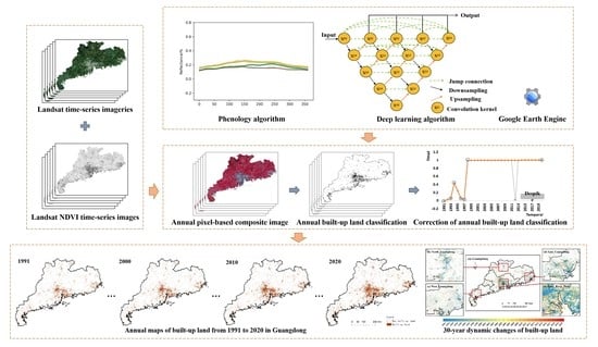
Annual Maps of Built-Up Land in Guangdong from 1991 to 2020 Based on Landsat Images, Phenology, Deep Learning Algorithms, and Google Earth Engine

1
College of Natural Resources and Environment, South China Agricultural University, Guangzhou 510642, China
2
Department of Microbiology and Plant Biology, University of Oklahoma, Norman, OK 73019, USA
3
Key Laboratory of Indoor Air Environment Quality Control, School of Environmental Science and Engineering, Tianjin University, Tianjin 300350, China
*
Author to whom correspondence should be addressed.
Remote Sens. 2022, 14(15), 3562; https://doi.org/10.3390/rs14153562
Submission received: 20 June 2022 / Revised: 19 July 2022 / Accepted: 20 July 2022 / Published: 25 July 2022
(This article belongs to the Special Issue Remote Sensing of Interaction between Human and Natural Ecosystem)

Abstract

:
Accurate mapping of built-up land is essential for urbanization monitoring and ecosystem research. At present, remote sensing is one of the primary means used for real-time and accurate surveying and mapping of built-up land, due to the long time series and multi-information advantages of existing remote sensing images and the ability to obtain highly precise year-by-year built-up land maps. In this study, we obtained feature-enhanced data regarding built-up land from Landsat images and phenology-based algorithms and proposed a method that combines the use of the Google Earth Engine (GEE) and deep learning approaches. The Res-UNet++ structural model was improved for built-up land mapping in Guangdong from 1991 to 2020. Experiments show that overall accuracy of built-up land map in the study area in 2020 was 0.99, the kappa coefficient was 0.96, user accuracy of built-up land was 0.98, and producer accuracy was 0.901. The trained model can be applied to other years with good results. The overall accuracy (OA) of the assessment results every five years was above 0.97, and the kappa coefficient was above 0.90. From 1991 to 2020, built-up land in Guangdong has expanded significantly, the area of built-up land has increased by 71%, and the proportion of built-up land has increased by 3.91%. Our findings indicate that the combined approach of GEE and deep learning algorithms can be developed into a large-scale, long time-series of remote sensing classification techniques framework that can be useful for future land-use mapping research.

Graphical Abstract

1. Introduction

The term “built-up land” refers to locations in which people engage in multiple social and economic activities [1,2]. These locations make use of the land’s carrying capacity or building space and are not used for the main purpose of obtaining biological products. Built-up land consists primarily of residential space, roads, public facilities, and parks that may include vegetation and scenic facilities. The change in built-up land is a slow and long process, and may not be complete if we only look at the change in built-up land in one or two years. Long-term monitoring and mapping can more accurately reflect dynamic changes in built-up land over long periods of time and reveal the temporal and spatial laws governing these changes. Amid rapid economic development and the acceleration of urbanization, large amounts of crop land and forest are occupied by built-up land, leading to a sharp decline in biodiversity and further adverse impacts. In particular, expansion affects the water cycle system, altering surface runoff and increasing the risk of waterlogging disasters [3,4], and aggravates the urban “heat island” phenomenon [5,6,7], contributing to ecosystem deterioration [8,9,10,11,12]. As such, the rate of change and trends in built-up land can directly or indirectly reflect and be used to evaluate the degree of urbanization. The swift acquisition of accurate spatial distribution information of built-up land supports analysis of changing trends in built-up land in the process of urban and rural development. This is crucial for formulating ecological and environmental protection policies, rationally planning land resources, and ensuring people’s quality of life [13].
Thanks to recent rapid developments in remote sensing technology, big data with high spatial resolution and temporal resolution are accumulating continuously, and long time series remote sensing images have become indispensable for the timely and accurate monitoring of built-up land. Several previous studies have explored the possibilities offered by remote sensing for identifying built-up land. These studies can be roughly divided into two classes: spectral analysis and image classification.
Spectral analysis can be simply understood as utilizing the spectral characteristics of remote sensing images to analyze and obtain specific information. Various built-up land indexes are available, including the Normalized Difference Built-up Index (NDBI) [14,15,16], the Index-based Built-up Index (IBI) [2,16,17,18], the Combinational Built-up Index (CBI) [16,19], the Modified Built-up Index (MBI) [16,19,20], and the Normalized Urban Areas Composite Index (NUACI) [14]. These index methods were relatively popular in early and even current spectral analysis research [21]. They can strengthen image features through calculations, and are then usually combined with the threshold method for the purpose of making judgments. The development of high-resolution images has allowed scholars to obtain built-up land characteristics based on dense time series image data using time series spectral analysis. For example, the spectral differences between impervious and pervious surfaces were analyzed from Landsat time series data [22]; time-space rules and Landsat time series stacks were used to capture continuous impervious surface dynamics [2]; MODIS NDVI and Landsat NDVI were merged for crop classification using long short-term memory (LSTM) algorithm [23]; and some scholars performed segment fitting on 12-year time series data and successfully extracted built-up land by extracting trajectory features [24]. In summary, spectral analysis can accomplish much using the spectral and temporal characteristic information provided by remote sensing images but cannot provide optimal accuracy for surveying and mapping long time series built-up land.
In contrast with spectral analysis, image classification involves the use of image segmentation technology to classify remote sensing images [25]. With the rapid development of image classification and segmentation technology, classification methods have evolved from decision tree classifiers and support vector machine (SVM) [18,26] methods to the more recent artificial neural network (ANN) [20,27,28] approach. Early research focused on simpler neural networks, such as random forests (RF) and back propagation (BP) neural networks. Zhang et al. [29] used multi-temporal synthesis and relative radiation normalization methods to extract phenological information and then mapped the impervious surface of the Yangtze River Delta from 1984 to 2020 using the RF method. Wan et al. [30] proposed a method that combined BP neural networks and support vector data description to extracted impervious surfaces. As deep learning methods used in other fields, such as medicine and biology, have matured, they have found new applications in remote sensing recognition research. Since 2018, deep learning has been used to identify built-up land. Tan et al. [31] designed a double-stream convolutional neural network that combines complementary cues from high-resolution panchromatic and multispectral images for high-resolution built-up area recognition. Compared with the most advanced technology available hitherto, Tan’s method has higher overall accuracy (OA) and superior generalization ability. Sun et al. [32] began from different data sources and proposed a three-dimensional convolutional neural network (3D-CNN) method for extracting impervious surfaces from WorldView-2 and airborne LiDAR datasets. To extract feature information more comprehensively, Zeng et al. [33] combined and optimized the Resnet and U-Net models to identify airport land. Pixel-level spatial and spectral information are typically used first, followed by the use of texture and feature maps through a multi-scale convolution process. This enhances the identification of impervious surfaces. Image classification methods can provide the year-by-year feature recognition required by national land monitoring authorities and other departments. The principle is simple, and the law of feature change can also be further analyzed. However, the data used in most studies were manually selected first-phase images with superior quality over a single year. Further research is required to address the need for year-by-year data processing and assess how the time–space spectral information provided by remote sensing images may be fully utilized to generate higher-precision built-up land maps.
Several large-scale identification and research projects have focused on built-up land. For example, NUACI is a global 30-m urban land cover dataset from 1990 to 2010 produced using an algorithm based on Landsat images [14]. LUC is a 1-km land use cover dataset from 2015 in China based on multi-source remote sensing data, such as Landsat-8 and GF-2, combined with data obtained from field surveys and human–computer interaction interpretation, with a comprehensive evaluation accuracy greater than 90% [34]. The Annual Global Land Cover (AGLC) is a global 30-m land cover dataset from 2000 to 2015, based on one year of high-confidence land cover data; it used random forests to classify areas that change every two years, resulting in 15 consecutive years of land cover data [13]. Mainstream large-scale mapping methods are still based on pixel-based approaches, such as RF. Pixel-based methods are more efficient in terms of computing power; they are also highly sensitive to small objects and able to map in greater detail. However, due to the complexity of mixed pixels and ground objects in remote sensing images, the results of pixel-based methods typically include “salt and pepper” noise.
To compensate for the above-mentioned shortcomings of existing research, we performed an analysis based on the following assumptions. First, the spectral differences in the remote sensing images captured across the period of a year differ significantly, and the artificial selection of one of these images is not scientifically sound. Remote sensing image classification is used primarily to obtain information from spectral features for classification. Therefore, we propose beginning from the spectral characteristics of different land uses, and then integrating all available images from a given year, and synthesizing feature-enhanced images for that year. Furthermore, to capture the dynamic changes in built-up land in a long-term series, it is necessary to perform year-by-year built-up land mapping. Similarly, the corrected outlier classification of mapping results should be based on long time series of annual results. Finally, year-by-year large-scale built-up land mapping research will inevitably involve problems related to processing, feature selection and training, and prediction of large sets of data. On one hand, deep learning identifies image features through neural networks and automatically filters image features through labels. This can significantly save computational power and time, and to a certain extent, minimize reliance on professional knowledge and experience. The Convolutional Neural Network (CNN) approach involves learning and predicting based on pixel blocks, which can take into account the context information of pixels, avoiding the problem of “salt and pepper” noise. On the other hand, big data can be accessed and analyzed quickly and easily on the Google Earth Engine (GEE) platform, which is provided by Google for online visualization, calculation, analysis, and processing of large amounts of large-scale earth science data (especially satellite data). GEE is supported by numerous parallel servers, so it has significant advantages in data sourcing and processing efficiency.
In conjunction with what was discussed above, in this study all available Landsat time-series imagery data were integrated to synthesize yearly feature-enhanced data with a phenology-based algorithm. Then, we combined the advantages of deep learning and GEE to train a built-up land model that enables fast and accurate identification of built-up land. Finally, we obtained and corrected the annual built-up map of Guangdong from 1991 to 2020, and analyzed the spatial and temporal distribution of built-up land in Guangdong for 30 consecutive years. The main objective of this study was to generate a large-scale, long-term and accurate dataset of 30 m built-up land in Guangdong from 1991 to 2020 by combining time-series Landsat imagery, phenology-based algorithm, deep learning methods, and GEE.

2. Material and Methods

2.1. Study Area

Guangdong is a provincial-level administrative region of the People’s Republic of China. According to the 2018 China Statistical Yearbook, Guangdong has an area of approximately 179,710 km2. Guangdong has been China’s most populous and largest economic province since 1989. In tandem with its economic development, land use in Guangdong has also witnessed drastic changes as the area of built-up land continues to increase. Moreover, the types and the distribution characteristics of its built-up land vary across different regions, making it a particularly suitable candidate for the study of built-up land identification.
As shown in Figure 1, Guangdong is divided into four sub-regions: West Guangdong, North Guangdong, East Guangdong, and the Pearl River Delta. Of these, the Pearl River Delta is Guangdong’s most prosperous region. It is also one of China’s three most densely populated and robust urban agglomerations.

2.2. Data and Pre-Processing

2.2.1. Landsat Imagery

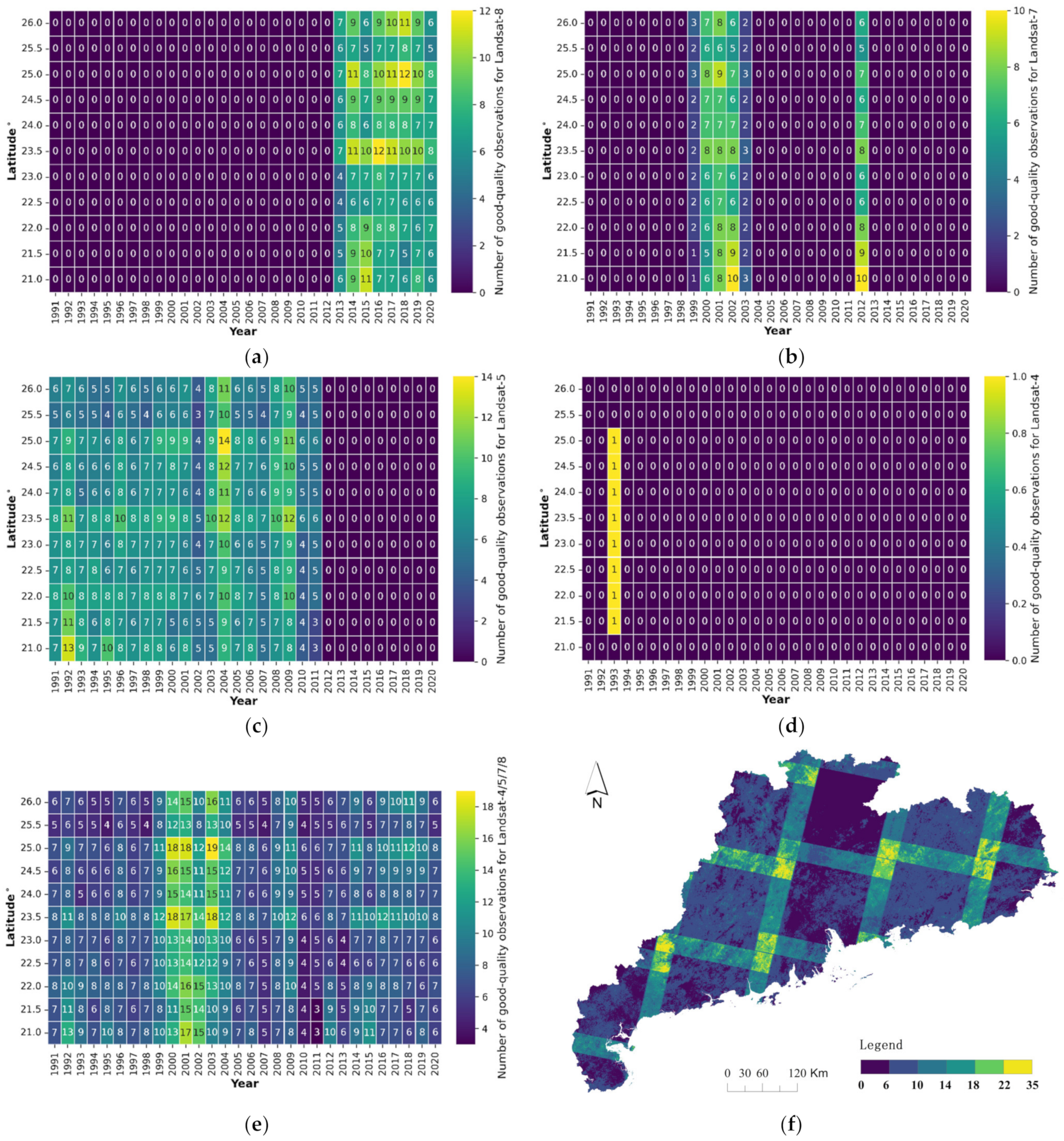
The data used in this study were obtained from GEE, and all data processing was implemented in GEE. We collected all available Landsat-4/5/7/8 surface reflectance (SR) data from 1991 to 2020. Table 1 shows the number of Landsat imagery used each year. Landsat-7 only used data from 1999 to 31 May 2003, due to the problematic presence of striping in the images, and data from 2012 (Landsat-8 has no available data from 2012). This dataset is the SR data from the Landsat 8 OLI/TIRS sensors, and had processed to the Level-1 Precision Terrain (L1TP) level. These data have been atmospherically corrected using Land Surface Reflectance Code (LaSRC, https://www.usgs.gov/media/files/landsat-8-collection-2-level-2-science-product-guide, accessed on 24 March 2022) and includes a cloud, shadow, water and snow mask produced using C implementation of mask function (CFMasK) [35], as well as a per-pixel saturation mask. The quality of Landsat SR data is determined by the “pixel_qa” band (a pixel quality attribute generated by the CFMask). To ensure high-quality observation data, cloud, cloud confidence, cirrus confidence, cloud shadow, snow/ice, and water were filtered by “pixel_qa” band (Figure 2).

2.2.2. Vegetation Index

Numerous studies have demonstrated that the Normalized Difference Vegetation Index (NDVI) is useful in identifying built-up land [34,36,37]. Moreover, NDVI is highly sensitive to green vegetation, which typically surrounds built-up land. To better extract built-up land boundaries, the NDVI of all valid data was calculated from Landsat SR data (Equation (1)) [38].
NDVI = NIR RED NIR + RED
where,
NIR = near infrared surface reflectance (851–879 nm) in Landsat imagery
RED = red surface reflectance (636–673 nm) in Landsat imagery

2.3. Algorithms for Identifying Time Series of Built-Up Land

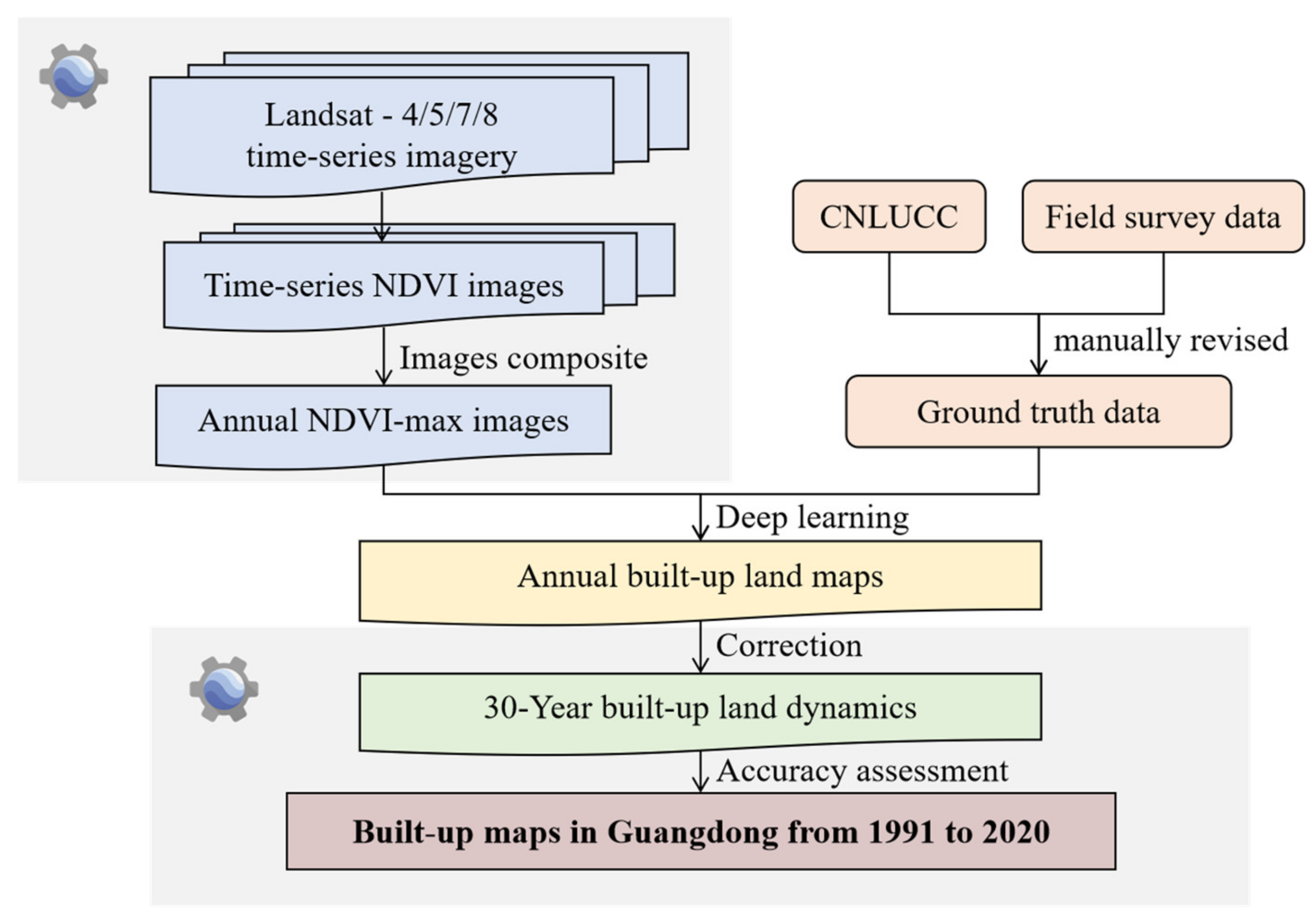
Figure 3 presents the workflow followed to map built-up land in Guangdong from 1991 to 2020. Based on all high-quality observations of the time series data collected, we synthesized the annual feature-enhanced data by analyzing the phenological spectral features of different land use types. Built-up land cover from 1991 to 2020 was predicted using deep learning techniques with ground truth data, and temporal segmentation was used to correct and generate 30-year spatiotemporal dynamics of the built-up land. Following accuracy assessing, built-up maps of Guangdong from 1991 to 2020 were produced. These methods are described in detail in the following sections.

2.3.1. Spectral Variability between Built-Up Land and Other Lands Based on Phenology

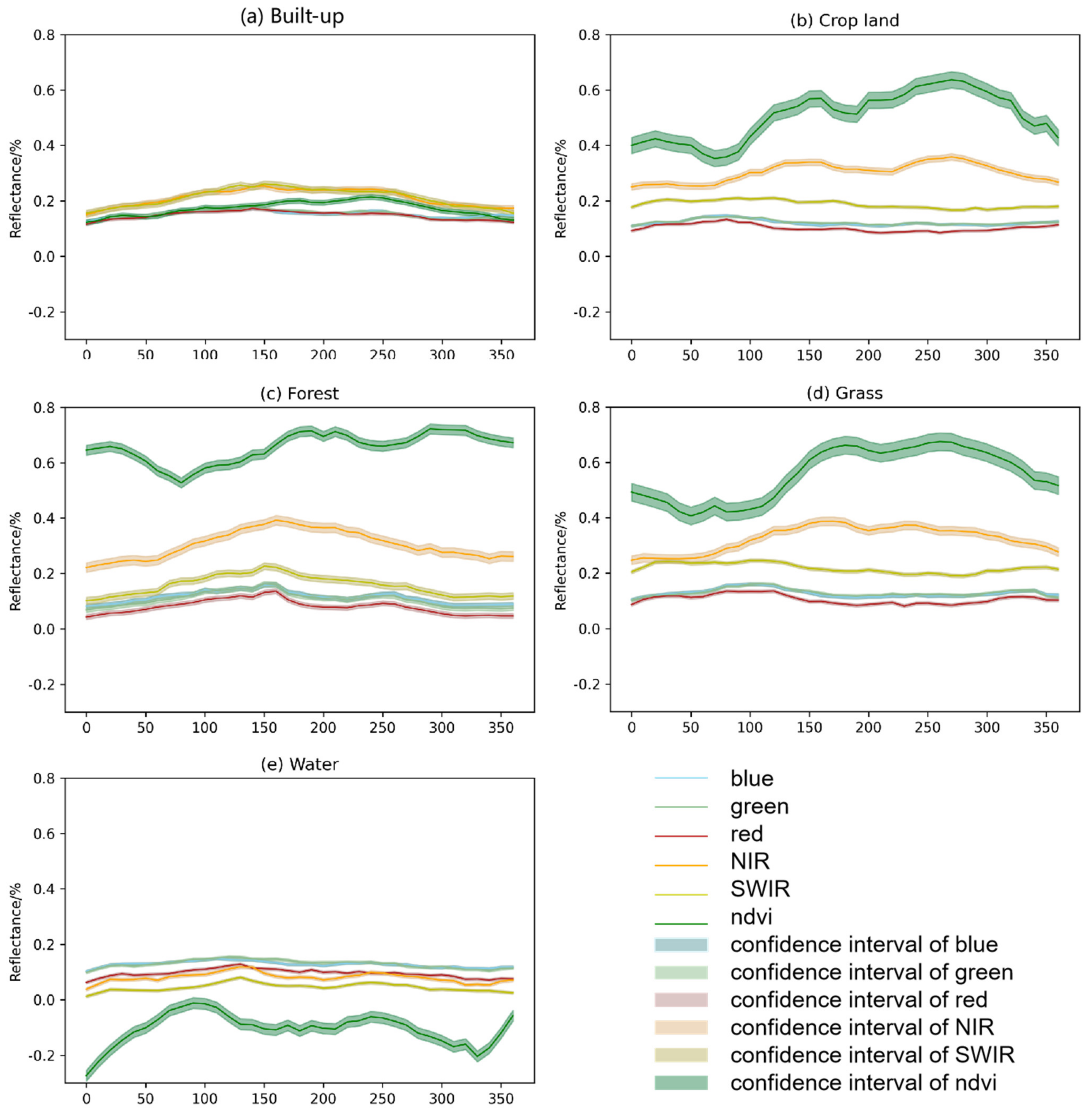
Forest, grassland, and cropland are typically covered by crops or vegetation during the lush growth period of the year, and bare during non-growth periods. Therefore, the spectral values usually differ significantly in the time series remote sensing images from a single year. The growth period also differs, as crop land in particular may undergo several growth periods. Compared with forest, grassland, and cropland, land covered by water is relatively stable, but the water may be covered by algae, so small fluctuations may be observed. Data for built-up land use should be stable with no significant fluctuations across the one-year spectral curve. Based on this principle, it is not scientifically sound to select only one image from a given year [39].
To generate an annual effective characteristic data set of built-up land, we analyzed the time series spectral characteristics of different land use types. Figure 4 presents the time series spectral curves for different land use types. The NDVI of water is usually less than 0 (Figure 4b); the NDVI of forest, cropland, and grassland is usually higher, and concentrated at 0.3–0.8 (Figure 4c–e); and the NDVI of built-up land is typically 0.1–0.3 (Figure 4a), which is smaller than the values for forest, cropland, and grassland and larger than water, which can be effectively distinguished. At the same time, built-up land is usually surrounded by vegetation, and the spectral information of mixed pixels also increasingly exhibits vegetation spectral characteristics [36]. In theory, therefore, NDVI can effectively distinguish built-up land from other land use types.

2.3.2. Annual Composite Feature Enhancement Images

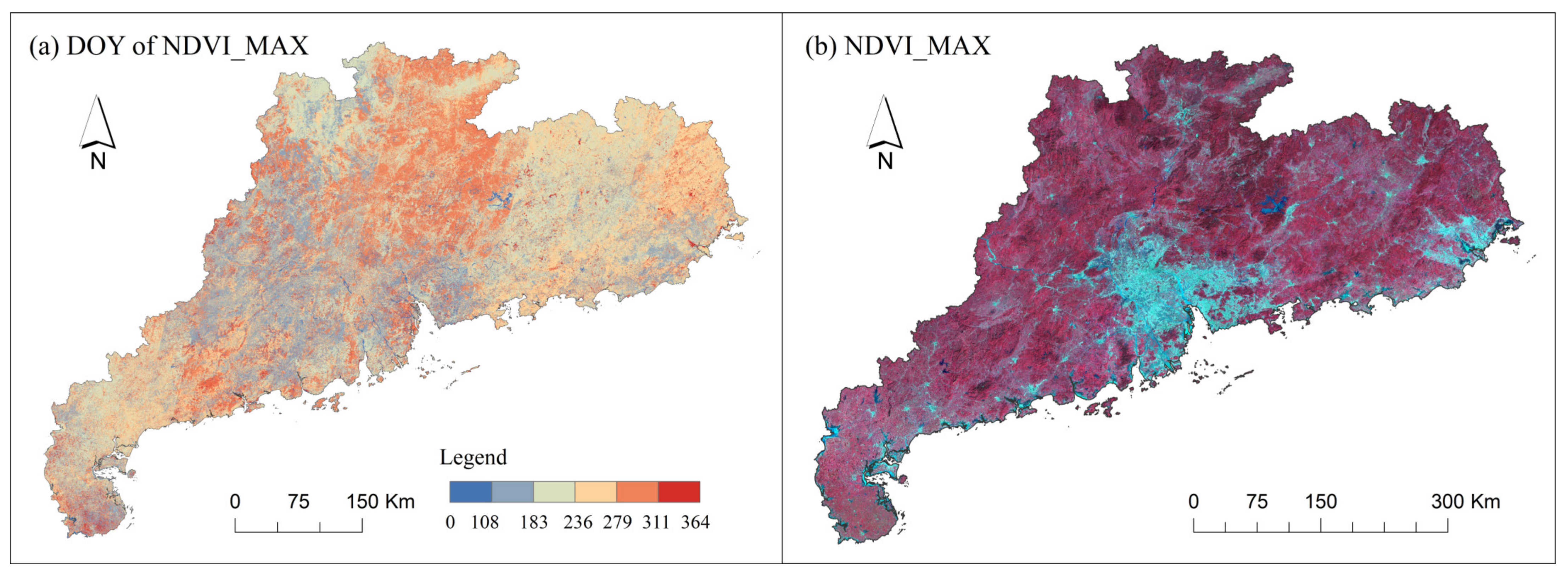
To enhance the data characteristics and improve the model training efficiency, we synthesized the valid data for each year. All images were composited in a collection, using a quality band as a per-pixel ordering function. Each pixel used the maximum value of NDVI as an index to compose the NDVI_MAX image per year [37] (Figure 5). In the annual NDVI_MAX images, blue (452–512 nm), green (533–590 nm), red (636–673 nm), NIR (851–879 nm), and SWIR-1 (1566–1651 nm) NDVI bands were selected as training bands, and some sample enhancement operations, such as random flip and rotation, were completed.

2.3.3. Deep Learning for Identifying Built-Up Land Per Year

Res-UNet++ Model for Identifying Built-Up Land

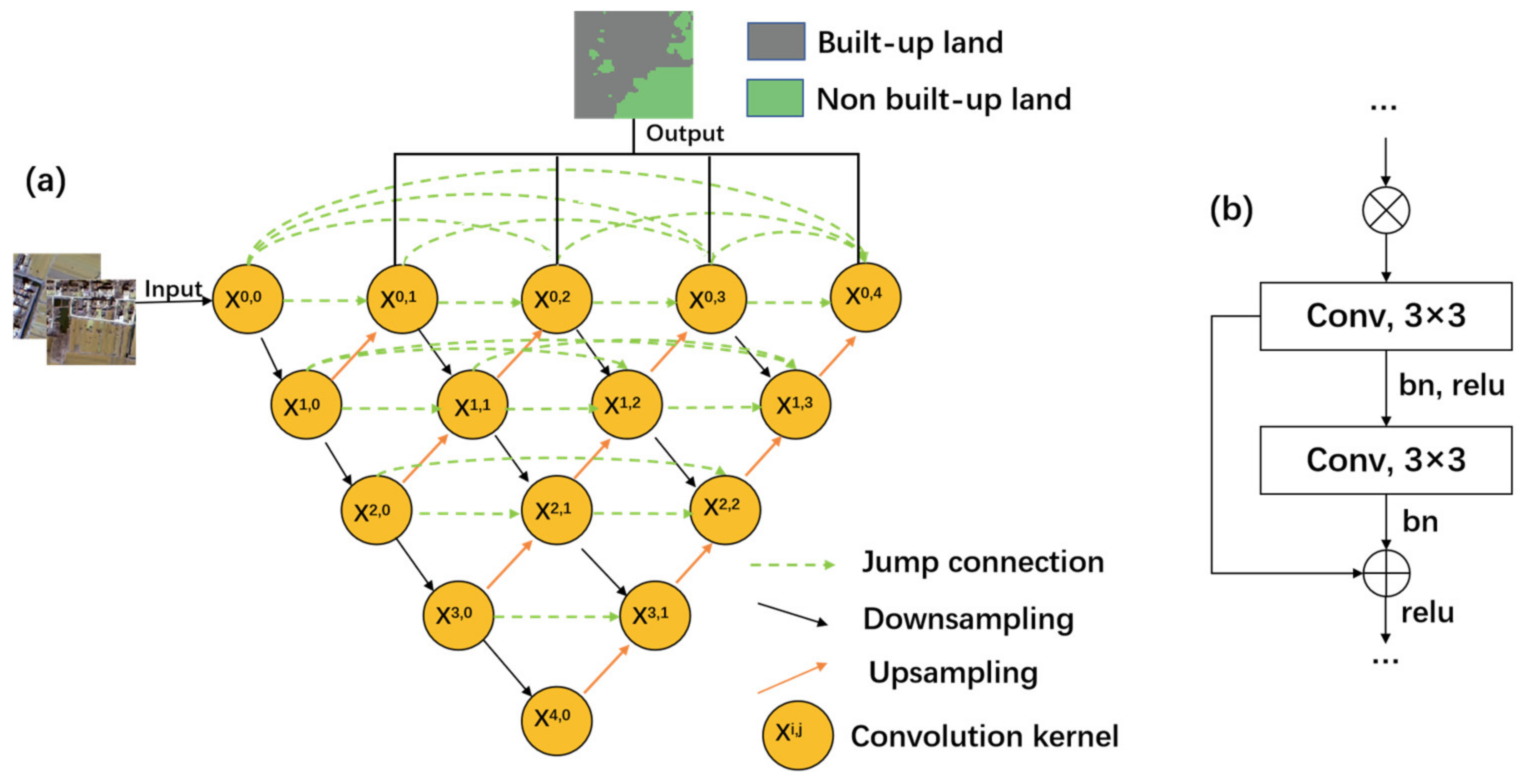
U-Net is a typical encoder–decoder structure network [40]. This model architecture can achieve good accuracy by training a smaller number of data samples, thereby reducing training time and resources. However, the feature maps obtained by the encoder in the traditional U-Net structure are directly superimposed with the decoder through skip connections. This will cause the network to lose a lot of information in the feature fusion part, affecting the mapping accuracy. Therefore, a dense jump connection is added between the encoder and the decoder—namely, U-Net++ [41]. This is considered an extension of U-Net, which can effectively reduce the semantic gap between low-level information and high-level information [42,43]. To address the problem of gradient disappearance or explosion during the U-Net structure training process, we introduced the residual structure design of Resnet to optimize our model [44], which became the Res-UNet++ model.
Figure 6a presents the structure of the Res-UNet++ model. Resnet18 residual structure was used as the backbone of Res-UNet++, as shown in Figure 6b. Each basic-block contained two 3 × 3 convolutions. Batch normalization layers were added to speed up the network learning, and maximum pooling was added to downsampling. Through this model structure, the features of each layer from shallow to deep in the encoder were connected and fused with the deep features in the decoder. The original image size of the feature was then restored by upsampling step by step.

Deeplab-v3 and FCN Models for Comparison

In the field of semantic segmentation, FCN [45] is a typical model, and Deeplab-v3 [46] has been applied very successfully in recent years. In this study, FCN and Deeplab-v3 were adopted for comparison with our Res-UNet++ and improved according to the characteristics of built-up land in the study area.
Figure 7a presents the architecture of Deeplab-v3. Xception was used as the backbone and Deeplab-v3 structure as the framework. Each encoder block was composed of 3 × 3 depthwise convolution, 1 × 1 pointwise convolution, batch normalization, and maximum pooling. Five encoder blocks were designed in total. In particular, atrous spatial pyramid pooling was added to the final step of downsampling, which is a module unique to Deeplab-v3. We applied atrous convolution to the cascade module to realize Atrous Spatial Pyramid Pooling (ASPP) [47]. On one hand, atrous convolution can address the problem of information loss caused by pooling, and the receptive field was increased without increasing the number of parameters to ensure that information was not lost. On the other hand, increasing multi-scale parallelism can resolve the problem of simultaneous segmentation of differently sized objects.
Figure 7b presents the architecture of FCN. Vgg16 was used as the backbone, and convolution transpose was used for upsampling. Each block was composed of two convolutions and one pooling. Five blocks were designed in total.

Parameters and Design of Deep Learning Training

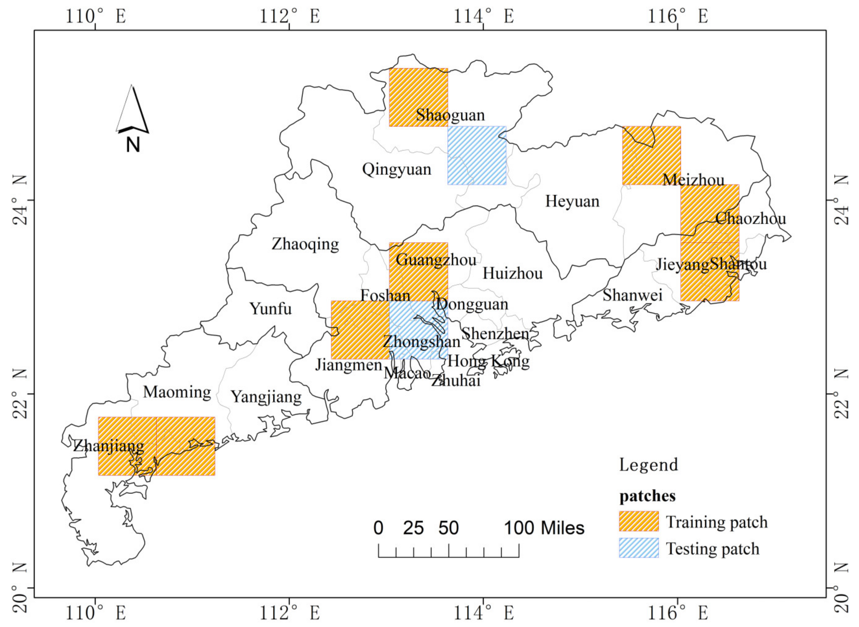
Due to the vastness of the research area, the production of label data based on the entire research area would be an enormous project. Therefore, the entire study area was divided using a 60 × 60-km grid. Two grids were selected as training data patches in each sub-region. The selection was based on the larger built-up land area and more built-up land types in the sub-regions, and the adjacent grid should be avoided as far as possible. To test the model’s generalization, two grids were selected as testing data patches in North Guangdong and Pearl River Delta (Figure 8).
Data from 2019 were used as training and validation data, and all ground truth data were produced through manual visual interpretation. The ground truth data were based on the China Multi-period Land Use Land Cover Change Remote Sensing Monitoring Dataset (CNLUCC, from the Resource and Environmental Science Data Registration and Publishing System), which was verified by field inspection and manually revised.
The learning rate adopted a piecewise constant decay strategy. The initial learning rate was 1 × 10⁻³, and the minimum learning rate is limited to 1 × 10⁻⁵. Learning rate was reduced by 5% when the accuracy difference between the two classes was very small. The model’s loss function set the sum of improved balanced binary cross-entropy loss and the dice coefficient loss [42]. The Adam optimization algorithm was used.

2.3.4. Correction of Time Series Built-Up Land by Temporal Segmentation Algorithm

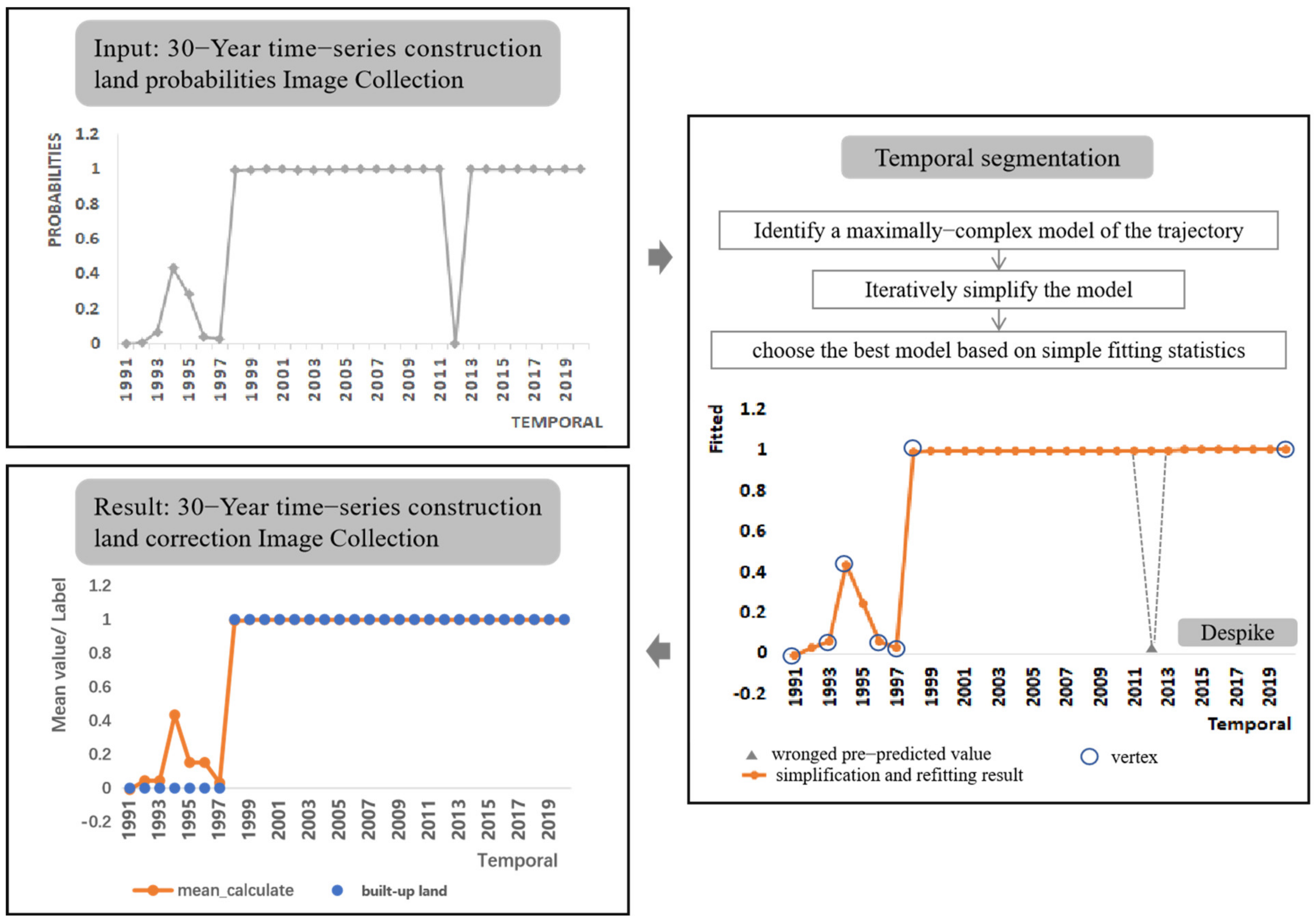
Due to the complexity of the built-up land system, some built-up land is temporarily occupied, and some non-built-up land is temporarily occupied for several years. To adapt to the long-term dynamic changes of built-up land, we attempted to correct the mapping results of built-up land year-by-year from the perspective of a longer time series.
We adopted LandTrendr (Landsat-based detection of Trends in Disturbance and Recovery) [48] to fit the long time series of built-up land probabilities to correct the misclassification of individual years. Figure 9 presents the pixel-based temporal smoothing procedure. The spectral time series of pixels were modeled as a linear segment sequence through temporal segmentation. Next, spikes with similar spectral values before and after the de-spiking algorithm were removed. Subsequently, the residual-error criterion was used to identify potential vertices, which had large deviations from the fitted regression line. We performed simplification and refitting based on vertices and simplifying models, and the final output of the segmentation algorithm emerged from the best model, which was determined using the p-value for the F-statistic.

2.4. Accuracy Assessment and Area Estimation

Validation data were selected and the area accuracy estimated following the “good practice” suggested by Olofsson [49].
Taking a Landsat pixel (30 × 30 m) as the evaluation unit, the stratified random sampling method was used to select the validation data based on four sub-regions. The sample size was based on the expected OA of the map and the assumed error matrix to obtain the approximate range, and the validation process was repeated to determine the best sample size [49]. We calculated the kappa coefficient [50] based on the confusion matrix and overall accuracy (OA), producer accuracy (PA), and user accuracy (UA) based on the error matrix. To ensure that the accuracy and area estimates were unbiased and consistent, we also estimated each standard deviation and confidence interval at 95%.
Since the research area is large and the sample weight is sufficient, the study area was stratified by sub-regions and map classes. The proportion of built-up land and non-built-up land was significantly unbalanced, so a combination of proportional and optimal distribution was adopted in the sample size allocation. After multiple experiments, 30 sample points for built-up land and 120 sample points for non-built-up land were obtained in each sub-region (Figure 10). According to the Landsat series imagery and the high spatial resolution Google Earth TM image, these samples were visually interpreted as reference data for accuracy assessment and area estimation. Assessment was completed every five years from 1991 to 2020.

3. Results

3.1. Model Comparison Experiment Result

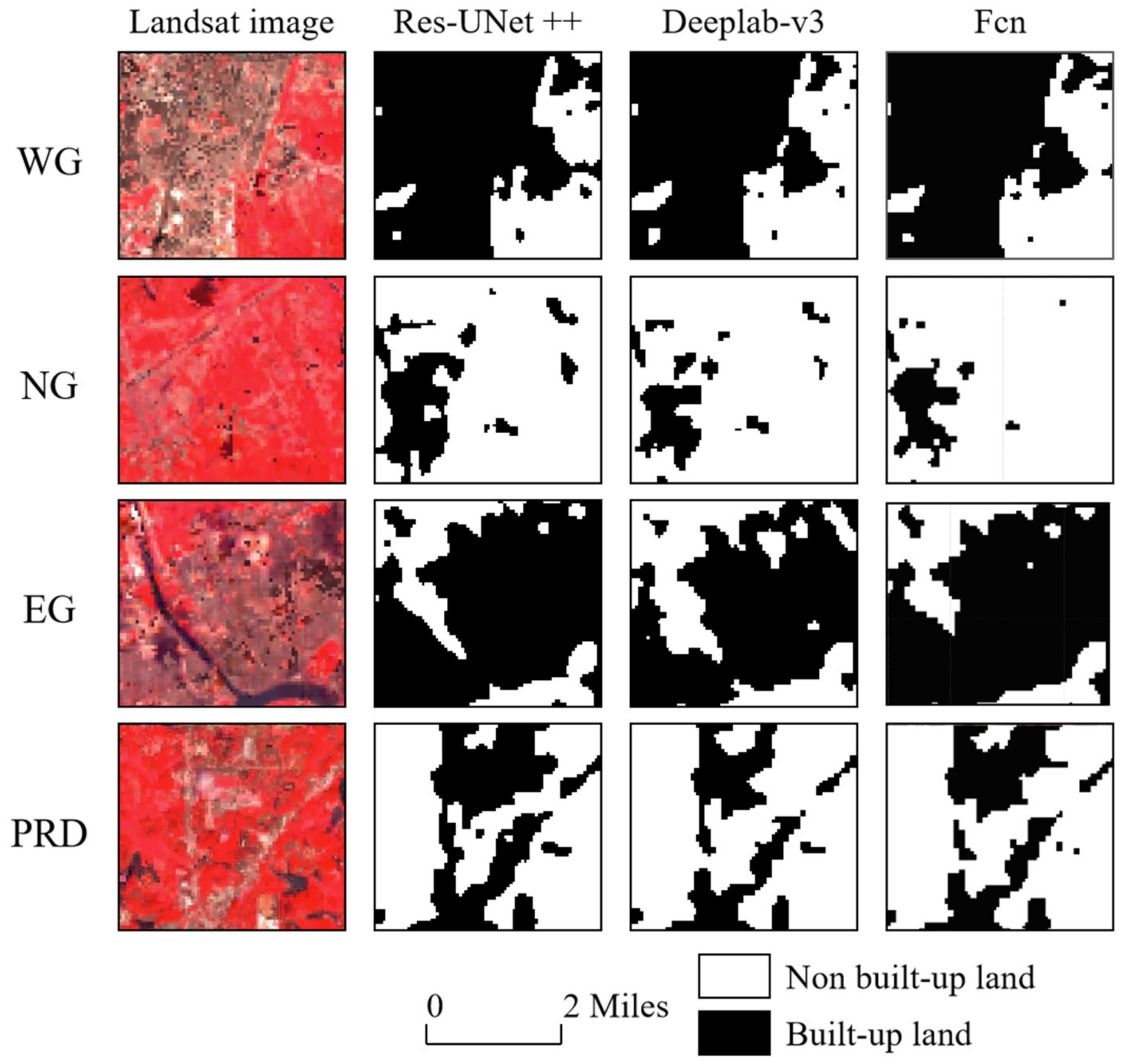
We used the improved Res-UNet++, Deeplab-v3, and FCN models to predict the built-up land map of Guangdong Province in 2020 and used the validation sample points for validation. Table 2 presents the comparison of each model’s accuracy. Res-UNet++ clearly yielded the highest accuracies: OA was 0.99, kappa was 0.96 in 2020, and UA and PA were also the highest among the three models. Among them, the PA of the BL in Res-UNet++ was considerably higher than that of the other two models. Accuracies of Deeplab-v3 and FCN were comparable: FCN was slightly higher on kappa and OA (OA was 0.95, kappa was 0.82 in 2020).
Figure 11 presents detailed comparisons of the mapping results of the three models. The main problem of Deeplab-v3 and FCN was the serious omission error of built-up land (PA of BL on Deeplab-v3 was 0.53, PA of BL on FCN was 0.55), which was mainly reflected in the rough identification of the built-up land boundary, and more omission errors could be expected in small areas of built-up land. As with the precision results, Res-UNet++ yielded the best results: it provided the best results for the identification effect of the built-up land boundary, and also provided the best results in mapping small areas of built-up land and the capture and judgment of spatial context information; in other words, it yielded the best semantic segmentation effects.
Table 3 summarizes the accuracy results of sub-regions according to the results of Res-UNet++, which was convenient for further analysis and comparison of regions in Guangdong. In general, the accuracies of each of the four sub-regions were relatively similar. The accuracy indicators of WG, NG, and PRD were almost identical, and the OA of EG was relatively low. The main reason for this was that the PA of built-up land was low, so omission errors were present, and from the accuracies of four sub-regions, the PA of built-up land was also lower than other accuracy values.

3.2. Assessment of Built-Up Land Maps from 1991 to 2020

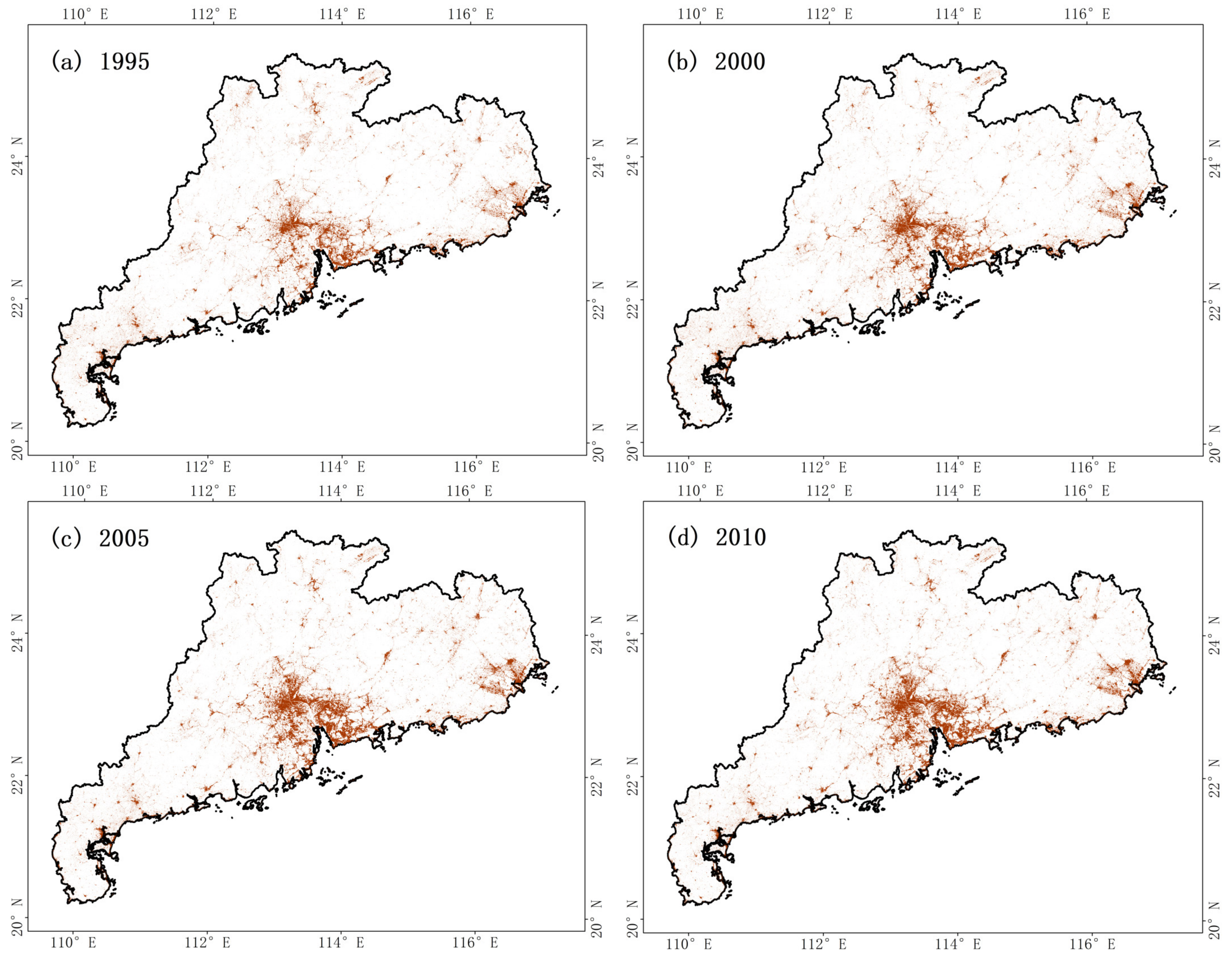
The built-up land mapping model was trained using the 2019 training patches. Based on this model, we predicted the built-up land map for each year from 1991 to 2020. The built-up land maps were displayed every five years, as shown in Figure 12. Table 4 lists the accuracy assessment, area estimation, and 95% confidence interval of area.
From the accuracy assessment in Table 4, we can see that OA peaked at 0.99 (2010) with a lowest value of 0.98 (2005); the kappa value peaked at 0.96 (2020) and had a lowest value of 0.94 (2010). Overall, the accuracies in 1995 and 2005 were lower than those in other years (OA was 0.98 and kappa was 0.90 in 1995; OA was 0.98 and kappa was 0.91 in 2005), mainly due to UA (0.93 in 1995; 0.94 in 2005) and PA (0.55 in 1995; 0.66 in 2005) in the built-up land class; 2020 had the highest accuracies (0.99 for OA and 0.96 for kappa).
From the spatial distribution of the built-up land maps in Figure 12 and the estimated built-up land area in Table 4, it is clear that there was an obvious phenomenon of built-up land expansion centered on towns and cities. Overall, the area of built-up land increased from 4.98 (±0.94) × 103 km2 in 1995 to 10.65 (±1.56) × 103 km2 in 2020. Among these, the greatest increase occurred between 2000 and 2005 (an increase of 1.56 × 10³ km2). Figure 12b,c shows that the most obvious built-up land expansion occurred in the PRD and EG. The second most obvious expansion was between 2015 and 2020 (an increase of 1.48 × 10³ km2), with an obvious expansion of built-up land at the village and town scale. The expansion of urban built-up land in the PRD region was also prominent. The smallest increase occurred between 1995 and 2000 (an increase of 390 km2), followed by between 2005 and 2010 (an increase of 940 km2).

3.3. Spatial-Temporal Changes of Built-Up Land in Guangdong

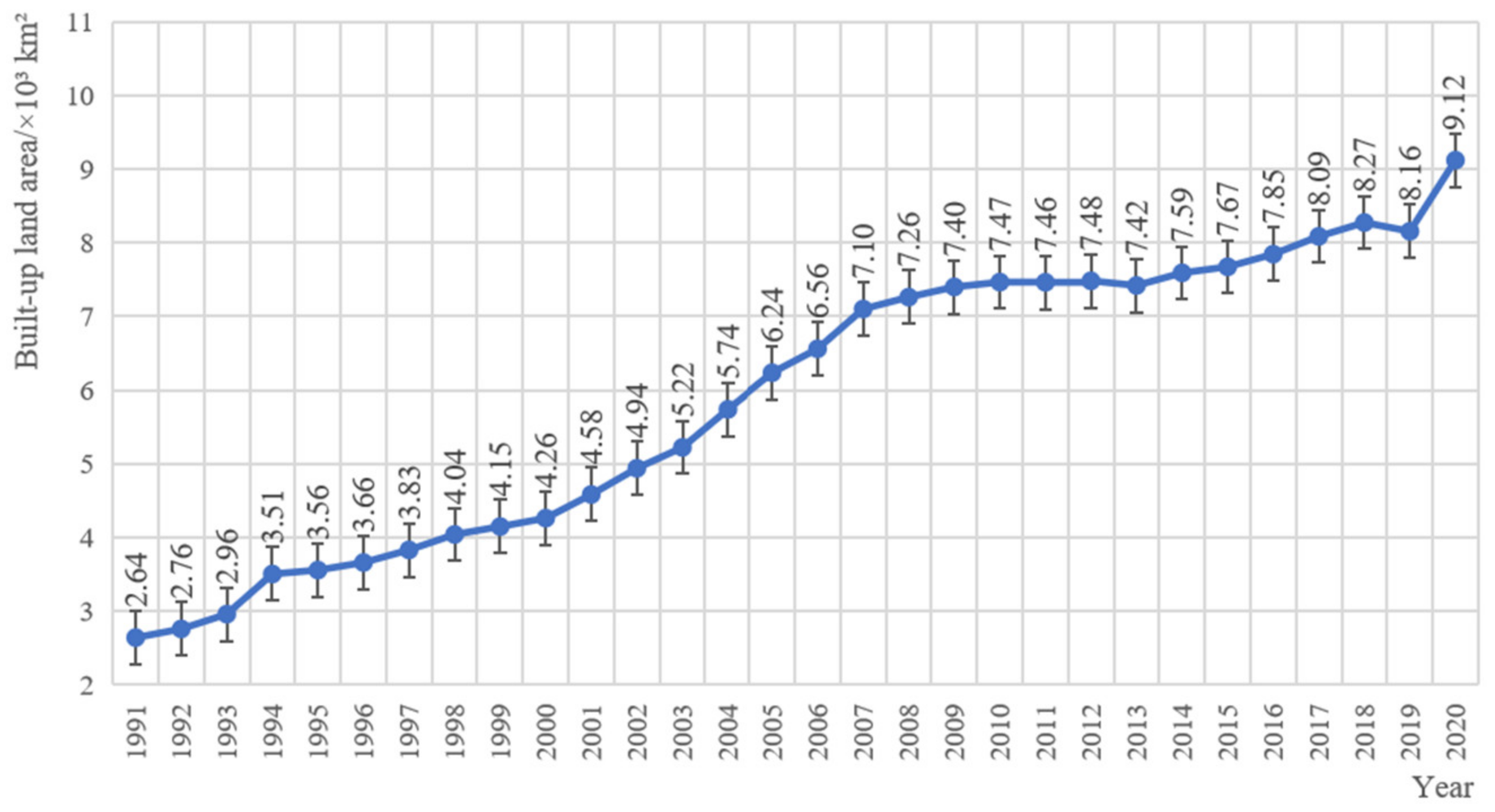
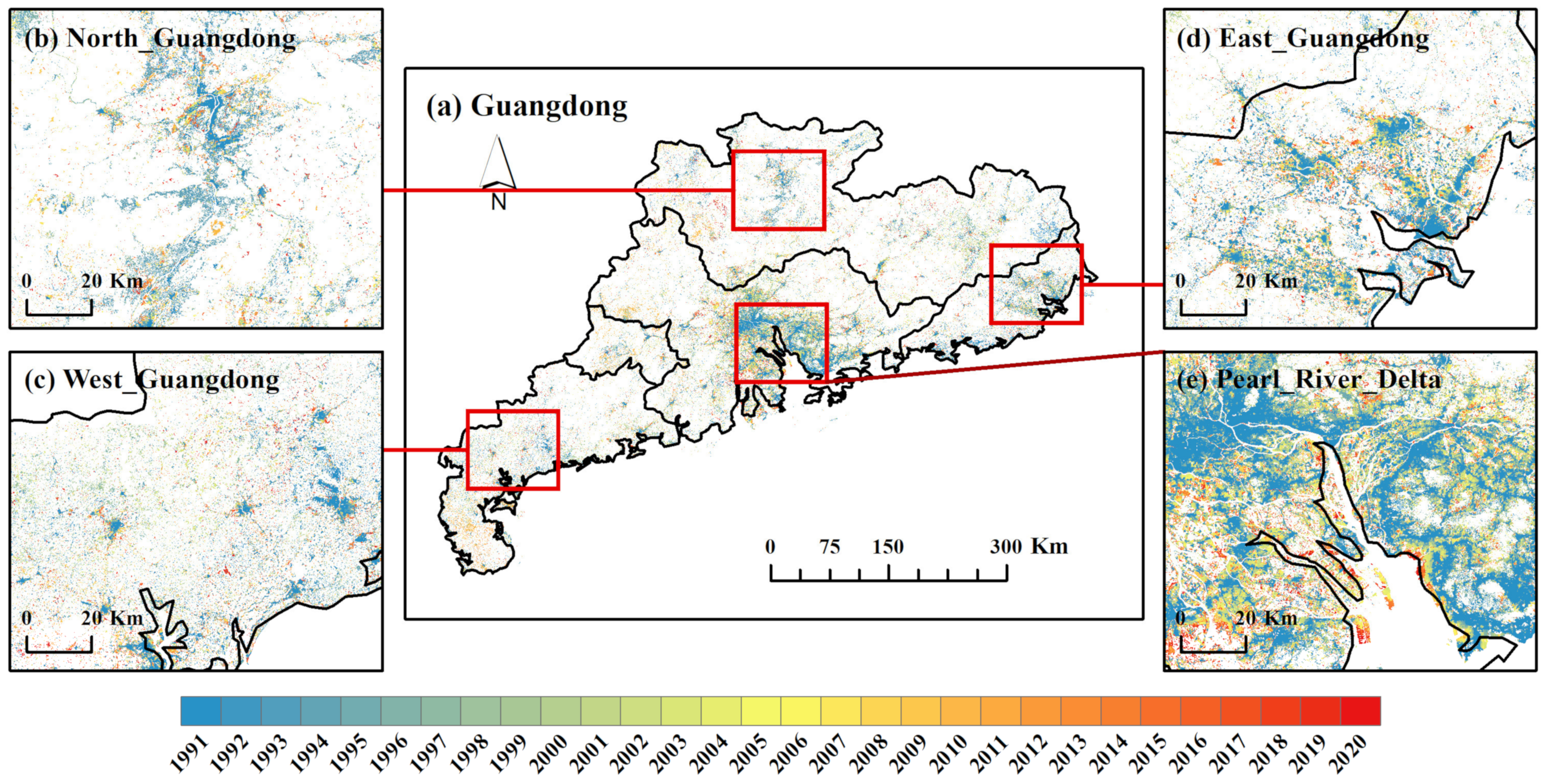
We counted the built-up land area mapped each year, as shown in Figure 13. Figure 14 presents the spatial distribution of built-up land expansion in Guangdong from 1991 to 2020. As shown in Figure 13, the built-up land did not increase every year: for example, it decreased by 60 km2 in 2012 and by 110 km2 in 2018, but on the whole, the built-up land in Guangdong expanded significantly, increasing from 2.64 × 10³ km2 in 1991 to 9.12 × 10³ km2 in 2020. The greatest expansion was 960 km2 in 2019, followed by 540 km2 in 1993 and 2006. Over a 30-year period, the built-up land increased by 71%. The proportion of built-up land in Guangdong has increased from 1.68% in 1991 to 5.59% in 2020–an increase of 3.91%.
From the perspective of regional spatial distribution, PRD had the largest area of built-up land and the fastest increase; WG had the smallest area and the slowest increase. PRD’s increase was concentrated in the Guangzhou-Dongguan-Shenzhen-Foshan urban agglomeration and was mainly due to the outward expansion of urban built-up land, which expanded faster in 2005 and 2020 (Figure 14e). The built-up land in EG was concentrated in the Chaoshan area (Shantou-Jieyang-Chaozhou-Shanwei). It was mainly urban built-up land that was expanding, with faster expansion rates in 2000 and 2005 (Figure 14d). The built-up land in NG was relatively scattered. The expansion mainly affected town built-up land, with faster expansion rates in 1995 and 2020 (Figure 14b). The built-up land in WG was relatively scattered and located mainly in villages and towns; it expanded most rapidly in 2020 (Figure 14c).

4. Discussion

4.1. Algorithms for Mapping Annual Built-Up Land Maps

In early built-up land mapping research, it was common to artificially select the best quality scene data for mosaicking [16,36] and calculate the indexes [36,51,52]. To maximize the advantages of existing time series images and highlight the spectral characteristics of built-up land, we synthesized the annual pixel-based NDVI maximum data as feature-enhanced data using all available time series data based on a phenology-based algorithm. The mapping results also verified that the NDVI_MAX data can reflect and highlight the characteristics of built-up land to a certain extent and can be used as basic data for built-up land mapping.
Res-UNet++, Deeplab-v3, and FCN structures were used in this study (Section 2.3.3), and the improved Res-UNet++ model was the best among these three models. Deeplab-v3 and the FCN structural model that we designed were not sufficient to extract built-up land details with a spatial resolution of 30 m, but the Res-UNet++ structural model can yield good results. These findings are sufficient to verify that the Res-UNet++ model we designed can effectively extract built-up land from large-scale 30-m spatial resolution remote sensing images. Moreover, the training rate of a built-up land mapping model in Guangdong was 1.80 × 10³ km2/s, enabling it to achieve good results and be applied to long-term series mapping. Therefore, we can also conclude that the deep learning method can efficiently identify built-up land in large-scale remote sensing images.
In earlier attempts at built-up land mapping, bare land, sandy land, and mixed pixels were commonly confused with built-up land [15,22,37]. In our built-up land maps, we also counted a matrix showing the specific situations of all commission errors in the built-up land map from 2020, as detailed in Table 5, and Figure 15 presents a detailed map of all misclassifications in 2020. We can see that three of the 120 built-up land validation points were misclassified (Figure 15B): the actual land uses of these three points are bare land, mixed pixels, and cropland. However, the level of commission error is still acceptable. In particular, our method had no commission error for sand, and the commission error for crop land was actually rare. The more serious commission error was the case in which bare land was classified as built-up land. Some omission errors also emerged in our mapping results (Figure 15A). This phenomenon was more prominent on some small areas of built-up land or branch roads. Since our method was implemented based on pixel blocks (such as 3 × 3 pixel blocks), some details could not be captured. Therefore, the built-up land area counted by our mapping results should be smaller than the actual area. These shortcomings may be addressed in future research.
Finally, we used the LandTrendr algorithm (Section 2.3.4) to re-fit the time series as post-processing. The results demonstrated that this method is suitable for post-processing of time series mapping, which can not only remove some simple errors but can also handle some complex situations. For example, due to the mixed pixels, the identification result of one pixel for three consecutive years was built-up land—non-built-up land—built-up land. LandTrendr can observe and judge results from longer time series. Some problems occurred with data due to cloud occlusion, and a small portion of water was mapped as built-up land over several years. These classifications will be reprocessed as built-up land. Temporal filtering improved the accuracy of the results.

4.2. Comparison with Different Datasets

To better reflect the quality of mapping data, the built-up land identification results in 2015 (DL-based_2015) were compared with NUACI_2015 [14], LUC_2015 [34], and AGLC_2015 [53]. Figure 16 compares four regions: the selected cities are relatively developed large cities or megacities, so the built-up land was concentrated and large. Overall, the spatial distribution of built-up land presented by the four data products was relatively consistent. The built-up land distribution of PRD was highly concentrated and contiguous, while the built-up land of WG had the spatial characteristics of scattered small areas.
Specifically, NUACI_2015, LUC_2015, and AGLC_2015 were pixel-based data products and were thus highly sensitive to the identification of tiny features. However, because the identification of NUACI_2015 was urban land, the identification of rural built-up land was lacking compared with other data, and the identification of built-up land should be the lowest. LUC_2015 was able to identify built-up land based on historical land use vector data and the human–computer interaction interpretation method, so the spatial distribution of the identified built-up land was relatively accurate, but the boundary was relatively rough. AGLC_2015 was highly sensitive to the identification of small roads and small areas of built-up land, and the identification was highly detailed. In contrast with the impervious surface identified by AGLC_2015, the data used in this study (DL-based_2015) identified built-up land. Due to the different definitions of identification objects, DL-based_2015 can identify areas such as urban wetlands and urban green spaces as built-up land, but impervious surfaces are not allowed. We also adopted the CNN method to realize identification based on pixel blocks. Therefore, our method focuses more on the extraction of spatial context information, with the result that the built-up land mapping was more comprehensive.
In sum, the data products obtained using different methods have different characteristics and different applications. In future research, appropriate methods can be selected according to different needs.

4.3. Advantages of Combining GEE and Deep Learning Methods

On one hand, GEE offers considerable advantages for the acquisition and processing of large amounts of data. Large amounts of free, high-quality data with different spatial and temporal resolutions are available via the GEE platform, which allowed us to directly acquire and process the data in parallel on GEE. In fact, it took only about 25 min to synthesize 30 years of annual NDVI_MAX data in Guangdong Province, which greatly reduced time and labor costs. Additionally, the algorithm of temporal smoothing had also been integrated on the GEE platform, which was convenient and fast to use. Therefore, batch data processing of large data volumes can be easily implemented using GEE.
On the other hand, deep learning has significant advantages in terms of data feature selection and feature learning. Deep learning simulates human brain neurons through complex neural networks to recognize and learn data features. In particular, CNNs are widely used in remote sensing image classification [20,31,33]. The relationship between time, space, and spectrum can be automatically discovered through convolution. This considerably reduces the manual selection features in the identification of built-up land, making it more intelligent and automated.
We combined GEE and deep learning methods: we used the cloud to process data on GEE and used GEE data for deep learning training, and the trained model could also be directly utilized and predicted on GEE, saving space, memory, and time. Real-time map display can also be performed on GEE, and the model’s shortcomings can be found over time. GEE has led to a new era of cloud operation, and the combination of GEE and deep learning will likely become the main method used in remote sensing mapping research.

4.4. Implications and Future Work

Mastering the spatial distribution of the temporal and spatial changes of built-up land over a period of 30 consecutive years helps support land planning and dynamic management of land resources. It is a necessary prerequisite to ensure the scientific implementation of spatial planning [1]. The phenology-based algorithm based on time series remote sensing images obtains characteristic image data by selecting unique spectral or phenological features, which can be applied to other land use classifications and even remote sensing interpretation work. The combination of this algorithm, GEE, and deep learning methods has developed into a large-scale, long-term series of remote sensing classification technology framework that will be useful for future land use mapping research.
In future research, we will apply the algorithm generalization to the built-up land mapping of the entire country as well as on a global scale in a longer time series. Theoretically, the algorithm of this study can be directly applied and implemented. However, the edge detection effect and detail effect of deep learning convolutional neural networks need to be optimized.

5. Conclusions

We proposed a method combining phenology-based algorithm, GEE, and deep learning to map annual built-up land from medium-resolution remote sensing images. This method used 30-m spatial resolution time series remote sensing images to generate pixel-based annual NDVI maximum images as feature enhancement data on GEE. Taking China’s Guangdong Province as the study area, the Res-UNet++ model with the U-Net++ structure as the backbone and Resnet18 as the framework was largely improved. Temporal segmentation was performed with the time series data of built-up land identification results. The accuracy of built-up land mapping was improved in various aspects, and we were able to map built-up land in Guangdong from 1991 to 2020. The results of our experiments indicate that our algorithm can identify built-up land relatively broadly and comprehensively, but the recognition effect needs to be improved in small area of built-up land. At the same time, the combination of the phenology-based algorithm, GEE, and deep learning offers significant advantages in data processing, feature learning, and model prediction efficiency and can be applied to long-term, large-scale remote sensing rapid identification research.

Author Contributions

Conceptualization, L.L. and H.X.; methodology, L.L. and H.X.; software, L.L.; validation, H.X., X.X. and Y.Q.; formal analysis, H.X., Z.Q. and X.X.; investigation, Z.Q.; resources, Y.Q., Z.Q., S.L. and X.T.; data curation, H.X. and L.L.; writing—original draft preparation, H.X.; writing—review and editing, H.X., X.X., Y.Q., Z.Q., S.L., X.T. and L.L.; visualization, H.X.; supervision, H.X. and L.L.; project administration, L.L. All authors have read and agreed to the published version of the manuscript.

Funding

This work was supported by the National Key Research and Development Program of China [grant number 2020YFD1100203].

Data Availability Statement

Not applicable.

Acknowledgments

The authors want to thank the editor, associate editor, and anonymous reviewers for their helpful comments and advice. This study was supported in part by the Data Registration and Publication System for Resources and Environmental Sciences (http://www.resdc.cn/DOI), DOI: 10.12078/2018070201, accessed on 2 July 2018.

Conflicts of Interest

The authors declare no conflict of interest.

References

  1. Hu, W.; Yang, Y.C.; Duan, Z.L. On Intelligent Extraction of Built-up land Based on High-resolution Satellite Image. Geol. Anhui 2014, 24, 210–212. [Google Scholar]
  2. Liu, C.; Zhang, Q.; Luo, H.; Qi, S.; Tao, S.; Xu, H.; Yao, Y. An efficient approach to capture continuous impervious surface dynamics using spatial-temporal rules and dense Landsat time series stacks. Remote Sens. Environ. 2019, 229, 114–132. [Google Scholar] [CrossRef]
  3. Weng, Q. Modeling Urban Growth Effects on Surface Runoff with the Integration of Remote Sensing and GIS. Environ. Manag. 2001, 28, 737–748. [Google Scholar] [CrossRef] [PubMed]
  4. Klöcking, B.; Haberlandt, U. Impact of land use changes on water dynamics––A case study in temperate meso and macroscale river basins. Phys. Chem. Earth Parts A/B/C 2002, 27, 619–629. [Google Scholar] [CrossRef]
  5. Lin, Y.S.; Xu, H.Q.; Zhou, R. A Study on Urban Impervious Surface Area and Its Relation with Urban Heat Island: Quanzhou City, China. Remote Sens. Technol. Appl. 2007, 22, 14–19. [Google Scholar]
  6. Arbuthnott, K.G.; Hajat, S. The Health Effects of Hotter Summers and Heat Waves in the Population of the United Kingdom: A Review of the Evidence. Environ. Health 2017, 16, 119. [Google Scholar] [CrossRef] [Green Version]
  7. Santamouris, M. Recent Progress on Urban Overheating and Heat Island Research. Integrated Assessment of the Energy, Environmental, Vulnerability and Health Impact. Synergies with the Global Climate Change. Energy Build. 2019, 207, 109482. [Google Scholar] [CrossRef]
  8. Arnfield, A.J. Two Decades of Urban Climate Research: A Review of Turbulence, Exchanges of Energy and Water, and the Urban Heat Island. Int. J. Clim. 2003, 23, 1–26. [Google Scholar] [CrossRef]
  9. Sarrat, C.; Lemonsu, A.; Masson, V.; Guédalia, D. Impact of Urban Heat Island on Regional Atmospheric Pollution. Atmos. Environ. 2005, 40, 1743–1758. [Google Scholar] [CrossRef]
  10. Weng, Q.; Lu, D. A sub-pixel analysis of urbanization effect on land surface temperature and its in-terplay with impervious surface and vegetation coverage in Indianapolis, United States. Int. J. Appl. Earth Obs. Geoinf. 2008, 10, 68–83. [Google Scholar]
  11. Feizizadeh, B.; Blaschke, T. Examining Urban Heat Island Relations to Land Use and Air Pollution: Multiple Endmember Spectral Mixture Analysis for Thermal Remote Sensing. IEEE J. Sel. Top. Appl. Earth Obs. Remote Sens. 2013, 6, 1749–1756. [Google Scholar] [CrossRef]
  12. Čeplová, N.; Kalusová, V.; Lososová, Z. Effects of Settlement Size, Urban Heat Island and Habitat Type on Urban Plant Biodiversity. Landsc. Urban Plan. 2017, 159, 15–22. [Google Scholar] [CrossRef]
  13. Xu, R.; Qu, R.; Liu, X.L.; Ma, H.R.; Shi, Z.T. Study on Impervious Surface Identification Method and Its Application Based on Sentinel-2 Data. Geogr. Geo-Inf. Sci. 2021, 37, 31–37. [Google Scholar]
  14. Liu, X.P.; Hu, G.H.; Chen, Y.M.; Li, X.; Xu, X.C.; Li, S.Y.; Pei, F.S.; Wang, S.J. High-resolution multi-temporal mapping of global urban land using Landsat images based on the Google Earth Engine Platform. Remote Sens. Environ. 2018, 209, 227–239. [Google Scholar] [CrossRef]
  15. Firozjaei, M.K.; Sedighi, A.; Kiavarz, M.; Qureshi, S.; Haase, D.; Alavipanah, S.K. Automated Built-Up Extraction Index: A New Technique for Mapping Surface Built-Up Areas Using LANDSAT 8 OLI Imagery. Remote Sens. 2019, 11, 1966. [Google Scholar] [CrossRef] [Green Version]
  16. Chen, J.; Chen, S.; Yang, C.; He, L.; Hou, M.; Shi, T. A comparative study of impervious surface extraction using Sentinel-2 imagery. Eur. J. Remote Sens. 2020, 53, 274–292. [Google Scholar] [CrossRef]
  17. Zhu, C.; Li, J.; Zhang, S.; Wu, C.; Zhang, B.; Gao, L.; Plaza, A. Impervious Surface Extraction from Multispectral Images via Morphological Attribute Profiles Based on Spectral Analysis. IEEE J. Sel. Top. Appl. Earth Obs. Remote Sens. 2018, 11, 4775–4790. [Google Scholar] [CrossRef]
  18. Zhang, L.; Zhang, M.; Yao, Y. Mapping seasonal impervious surface dynamics in Wuhan urban agglomeration, China from 2000 to 2016. Int. J. Appl. Earth Obs. Geoinf. ITC J. 2018, 70, 51–61. [Google Scholar] [CrossRef]
  19. Fang, H.; Wei, Y.; Dai, Q. A Novel Remote Sensing Index for Extracting Impervious Surface Distribution from Landsat 8 OLI Imagery. Appl. Sci. 2019, 9, 2631. [Google Scholar] [CrossRef] [Green Version]
  20. Zhang, T.; Tang, H. A Comprehensive Evaluation of Approaches for Built-Up Area Extraction from Landsat OLI Images Using Massive Samples. Remote Sens. 2019, 11, 2. [Google Scholar] [CrossRef] [Green Version]
  21. Abdelhady, H.U.; Troy, C.D.; Habib, A.; Manish, R. A Simple, Fully Automated Shoreline Detection Algorithm for High-Resolution Multi-Spectral Imagery. Remote Sens. 2022, 14, 557. [Google Scholar] [CrossRef]
  22. Zhang, L.; Weng, Q. Annual dynamics of impervious surface in the Pearl River Delta, China, from 1988 to 2013, using time series Landsat imagery. ISPRS J. Photogramm. Remote Sens. 2016, 113, 86–96. [Google Scholar] [CrossRef]
  23. Xie, Y.; Zhang, Y.; Xun, L.; Chai, X. Crop classification based on multi-source remote sensing data fusion and LSTM algorithm. Trans. Chin. Soc. Agric. Eng. 2019, 35, 129–137. [Google Scholar]
  24. Wang, B.; Chen, Z.; Zhu, A.-X.; Hao, Y.; Xu, C. Multi-Level Classification Based on Trajectory Features of Time Series for Monitoring Impervious Surface Expansions. Remote Sens. 2019, 11, 640. [Google Scholar] [CrossRef] [Green Version]
  25. Dominici, D.; Zollini, S.; Alicandro, M.; Della Torre, F.; Buscema, P.M.; Baiocchi, V. High Resolution Satellite Images for Instantaneous Shoreline Extraction Using New Enhancement Algorithms. Geosciences 2019, 9, 123. [Google Scholar] [CrossRef] [Green Version]
  26. Xi, Y.; Thinh, N.X.; Li, C. Preliminary comparative assessment of various spectral indices for built-up land derived from Landsat-8 OLI and Sentinel-2A MSI imageries. Eur. J. Remote Sens. 2019, 52, 240–252. [Google Scholar] [CrossRef] [Green Version]
  27. Deng, C.; Zhu, Z. Continuous subpixel monitoring of urban impervious surface using Landsat time series. Remote Sens. Environ. 2020, 238, 110929. [Google Scholar] [CrossRef]
  28. Zhu, Q.; Zhang, Y.; Wang, L.; Zhong, Y.; Guan, Q.; Lu, X.; Zhang, L.; Li, D. A Global Context-aware and Batch-independent Network for road extraction from VHR satellite imagery. ISPRS J. Photogramm. Remote Sens. 2021, 175, 353–365. [Google Scholar] [CrossRef]
  29. Zhang, X.; Liu, L.; Chen, X.; Gao, Y.; Jiang, M. Automatically Monitoring Impervious Surfaces Using Spectral Generalization and Time Series Landsat Imagery from 1985 to 2020 in the Yangtze River Delta. J. Remote Sens. 2021, 2021, 9873816. [Google Scholar] [CrossRef]
  30. Wan, Y.; Fei, Y.; Wu, T.; Jin, R.; Xiao, T. A Novel Impervious Surface Extraction Method Integrating POI, Vehicle Trajectories, and Satellite Imagery. IEEE J. Sel. Top. Appl. Earth Obs. Remote Sens. 2021, 14, 8804–8814. [Google Scholar] [CrossRef]
  31. Tan, Y.; Xiong, S.; Li, Y. Automatic Extraction of Built-Up Areas from Panchromatic and Multispectral Remote Sensing Images Using Double-Stream Deep Convolutional Neural Networks. IEEE J. Sel. Top. Appl. Earth Obs. Remote Sens. 2018, 11, 3988–4004. [Google Scholar] [CrossRef]
  32. Sun, Z.; Zhao, X.; Wu, M.; Wang, C. Extracting Urban Impervious Surface from WorldView-2 and Airborne LiDAR Data Using 3D Convolutional Neural Networks. J. Indian Soc. Remote Sens. 2019, 47, 401–412. [Google Scholar] [CrossRef] [Green Version]
  33. Zeng, F.; Wang, X.; Zha, M. Extracting built-up land area of airports in China using Sentinel-2 imagery through deep learning. Geocarto Int. 2021, 1–21. [Google Scholar] [CrossRef]
  34. Liu, J.Y.; Ning, J.; Kuang, W.H.; Xu, X.L.; Zhang, S.W.; Yan, C.Z.; Li, R.D.; Wu, S.X.; Hu, Y.F.; Du, G.M.; et al. Spatio-temporal patterns and characteristics of land-use change in China during 2010–2015. Acta Geogr. Sin. 2018, 73, 789–802. [Google Scholar]
  35. Foga, S.; Scaramuzza, P.L.; Guo, S.; Zhu, Z.; Dilley, R.D., Jr.; Beckmann, T.; Schmidt, G.L.; Dwyer, J.L.; Hughes, M.J.; Laue, B. Cloud Detection Algorithm Comparison and Validation for Operational Landsat Data Products. Remote Sens. Environ. 2017, 194, 379–390. [Google Scholar] [CrossRef] [Green Version]
  36. Feng, S.; Fan, F. A Hierarchical Extraction Method of Impervious Surface Based on NDVI Thresholding Integrated with Multispectral and High-Resolution Remote Sensing Imageries. IEEE J. Sel. Top. Appl. Earth Obs. Remote Sens. 2019, 12, 1461–1470. [Google Scholar] [CrossRef]
  37. Gong, P.; Li, X.; Zhang, W. 40-Year (1978–2017) human settlement changes in China refected by impervious surfaces from satellite remote sensing. Sci. Bull. 2019, 64, 756–763. [Google Scholar] [CrossRef] [Green Version]
  38. Tucker, C.J. Red and Photographic Infrared Linear Combinations for Monitoring Vegetation. Remote Sens. Environ. 1979, 8, 127–150. [Google Scholar] [CrossRef] [Green Version]
  39. Ablin, R.; Sulochana, C.; Prabin, G. An investigation in satellite images based on image enhancement techniques. Eur. J. Remote Sens. 2020, 53, 86–94. [Google Scholar] [CrossRef] [Green Version]
  40. Ronneberger, O.; Fischer, P.; Brox, T. U-Net: Convolutional Networks for Biomedical Image Segmentation. In Proceedings of the International Conference on Medical Image Computing and Computer-Assisted Intervention, Munich, Germany, 5–9 October 2015; pp. 234–241. [Google Scholar]
  41. Zhou, Z.; Md Mahfuzur Rahman, S.; Tajbakhsh, N.; Liang, J. UNet++: A Nested U-Net Architecture for Medical Image Segmentation. In Deep Learning in Medical Image Analysis and Multimodal Learning for Clinical Decision Support, Proceedings of the 4th International Workshop, DLMIA 2018, and 8th International Workshop, ML-CDS 2018, Granada, Spain, 20 September 2018; Springer Nature: Cham, Switzerland, 2018; Volume 11045, pp. 3–11. [Google Scholar]
  42. Peng, D.; Zhang, Y.; Guan, H. End-to-End Change Detection for High Resolution Satellite Images Using Improved UNet++23. Remote Sens. 2019, 11, 1382. [Google Scholar] [CrossRef] [Green Version]
  43. Jeong, M.; Choi, H.; Choi, J. Analysis of Change Detection Results by UNet++ Models According to the Characteristics of Loss Function. Korean J. Remote Sens. 2020, 36, 929–937. [Google Scholar] [CrossRef]
  44. Diakogiannis, F.I.; Waldner, F.; Caccetta, P.; Wu, C. ResUNet-a: A Deep Learning Framework for Semantic Segmentation of Remotely Sensed Data. ISPRS J. Photogramm. Remote Sens. 2020, 162, 94–114. [Google Scholar] [CrossRef] [Green Version]
  45. Long, J.; Shelhamer, E.; Darrell, T. Fully Convolutional Networks for Semantic Segmentation. IEEE Trans. Pattern Anal. Mach. Intell. 2017, 39, 640–651. [Google Scholar]
  46. Chen, T.-H.K.; Qiu, C.; Schmitt, M.; Zhu, X.X.; Sabel, C.E.; Prishchepov, A.V. Mapping horizontal and vertical urban densification in Denmark with Landsat time-series from 1985 to 2018: A semantic segmentation solution. Remote Sens. Environ. 2020, 251, 112096. [Google Scholar] [CrossRef]
  47. Chen, L.C.; Papandreou, G.; Kokkinos, I.; Murphy, K.; Yuille, A.L. DeepLab: Semantic Image Segmentation with Deep Convolutional Nets, Atrous Convolution, and Fully Connected CRFs. IEEE Trans. Pattern Anal. Mach. Intell. 2017, 40, 834–848. [Google Scholar] [CrossRef] [Green Version]
  48. Kennedy, R.E.; Yang, Z.; Cohen, W.B. Detecting trends in forest disturbance and recovery using yearly Landsat time series: 1. LandTrendr—Temporal segmentation algorithms. Remote Sens. Environ. 2010, 114, 2897–2910. [Google Scholar] [CrossRef]
  49. Olofsson, P.; Foody, G.M.; Herold, M.; Stehman, S.V.; Woodcock, C.E.; Wulder, M.A. Good practices for estimating area and assessing accuracy of land change. Remote Sens. Environ. 2014, 148, 42–57. [Google Scholar] [CrossRef]
  50. Fitzgerald, R.; Lees, B. Assessing the Classification Accuracy of Multisource Remote Sensing Data. Remote Sens. Environ. 1994, 47, 362–368. [Google Scholar] [CrossRef]
  51. Bouhennache, R.; Bouden, T.; Taleb-Ahmed, A.; Cheddad, A. A new spectral index for the extraction of built-up land features from Landsat 8 satellite imagery. Geocarto Int. 2019, 34, 1531–1551. [Google Scholar] [CrossRef]
  52. Li, C.; Wang, X.; Wu, Z.; Dai, Z.; Yin, J.; Zhang, C. An Improved Method for Urban Built-Up Area Extraction Supported by Multi-Source Data. Sustainability 2021, 13, 5042. [Google Scholar] [CrossRef]
  53. Xu, X.C.; Li, B.J.; Liu, X.P.; Li, X.; Shi, Q. Mapping annual global land cover changes at a 30m res-olution from 2000 to 2015. Natl. Remote Sens. Bull. 2021, 25, 1896–1921. [Google Scholar]
Figure 1. Study area.
Remotesensing 14 03562 g001
Figure 2. Good-quality observation of time-series remote sensing image from 1991 to 2020 according to the latitude. (ad) show the number of Landsat 4, 5, 7 and 8 each year for 30 years. (e) shows total numbers in all study areas. (f) shows the number of Guangdong in 2019 in the form of a map.
Remotesensing 14 03562 g002
Figure 3. Workflow of mapping built-up land in Guangdong province from 1991 to 2020.
Remotesensing 14 03562 g003
Figure 4. Time−series spectral curves for different land-use types with 1 data every 10 days were synthesized using all available Landsat−7, 8 and Sentinel-2 remote sensing imagery. The abscissa of the curve is the number of days in a year, and the ordinate is the reflectance of SR. (ae) represent the time−series spectral curves of built-up land, crop land, forest, grass and water, respectively.
Remotesensing 14 03562 g004
Figure 5. The feature enhancement data (NDVI_MAX) of the study area in 2019. (a) shows the Day of Year (DOY) each pixel of NDVI_MAX; (b) shows false color image of NDVI_MAX.
Remotesensing 14 03562 g005
Figure 6. The overall flowchart of the proposed Res-UNet++ model. (a) the main flowchart of Res-UNet++; (b) the flowchart of Resnet18 residual basic-block (bn-batch normalization layer, relu-the activation function, Conv-convolution layer.).
Remotesensing 14 03562 g006
Figure 7. The structure of the compared model. (a) the structure of Deeplab-v3; (b) the structure of FCN.
Remotesensing 14 03562 g007
Figure 8. Spatial distribution of training and testing patches.
Remotesensing 14 03562 g008
Figure 9. The procedure of pixel−based temporal smoothing.
Remotesensing 14 03562 g009
Figure 10. Spatial distribution of validation sample points.
Remotesensing 14 03562 g010
Figure 11. Examples of built-up land produced by Res-UNet++, Deeplab-v3 and FCN in 2020.
Remotesensing 14 03562 g011
Figure 12. Annual built-up land maps of Guangdong, China in 1995, 2000, 2005, 2010, 2015, 2020.
Remotesensing 14 03562 g012aRemotesensing 14 03562 g012b
Figure 13. Built-up land area and its standard error statistics in annual classification maps.
Remotesensing 14 03562 g013
Figure 14. Built-up land expansion in Guangdong from 1991 to 2020.
Remotesensing 14 03562 g014
Figure 15. Examples of classification errors in the mapping of built-up land in Guangdong in 2020. (A) Examples of omission errors; (B) all commission errors in 120 built-up land validation points.
Remotesensing 14 03562 g015
Figure 16. Comparison of built-up land mapping examples of three important data products in four sub-regions in 2015. DL-based_2015 is the data of this study, which identified built-up land; NUACI_2015 is the product of the global 30 m urban land; LUC_2015 is the product of the 1 km land use (built-up land) in China; AGLC_2015 is the product of the global 30 m land cover (impervious surface).
Remotesensing 14 03562 g016
Table 1. Number of Landsat imagery used totally each year.
YearNumberYearNumberYearNumberYearNumberYearNumber
19912671997271200342720093352015359
19922891998281200437720102102016371
19932251999368200527120111952017387
19942362000603200628520122022018394
19952502001585200723220132732019341
19962902002530200829720143722020352
Table 2. Accuracy assessment of built-up land maps based on Res-UNet++, Deeplab-v3 and FCN model in 2020 (BL-Built-up land, N-BL-Non-Built-up land).
ModelOAKappaUAPA
N-BLBLN-BLBL
Res-UNet++0.990.960.990.971.000.83
Deeplab-v30.940.780.930.971.000.53
FCN0.950.820.950.931.000.55
Table 3. Error matrix with cell entries expressed in terms of proportion of area and accuracies based on Res-UNet++ in 2020. The vertical axis represents the truth, and the horizontal axis represents the results of mapping, which are divided into four sub-regions for statistics (WG–West Guangdong, NG–North Guangdong, EG–East Guangdong, PRD–Pearl River Delta).
Sub-Regions Reference
N-BLBLTotalUA
WGMapN-BL0.94 0.01 0.950.99
BL0.000.05 0.05 0.97
Total0.940.061.00
PA1.000.86 OA = 0.99
NGMapN-BL0.940.010.95 0.99
BL0.000.050.05 0.97
Total0.940.06 1.00
PA1.000.86 OA = 0.99
EGMapN-BL0.930.020.950.98
BL0.000.050.051.00
Total0.930.0671.00
PA1.000.76 OA = 0.98
PRDMapN-BL0.940.010.950.99
BL0.000.050.050.97
Total0.94 0.061.00
PA1.00 0.86 OA = 0.99
Table 4. Accuracies assessment, area estimation and its 95% confidence interval in Guangdong in 1995, 2000, 2005, 2010, 2015 and 2020.
YearOAKappaUAPAArea (95% CI) (×103 km2)
BLN-BLBLN-BL
19950.980.900.930.990.551.004.98 (±0.94)
20000.990.920.940.990.631.005.37 (±1.76)
20050.980.910.940.980.661.006.93 (±1.02)
20100.990.940.940.990.851.007.87 (±0.71)
20150.980.930.970.980.731.009.17 (±1.90)
20200.990.960.970.990.831.0010.65 (±1.56)
Table 5. Statistical matrix of land use for all commission errors of built-up land in Guangdong in 2020. Among 120 BL validation sample points in Guangdong, 3 N-BL were mapped as BL, and the actual land types were counted.
RegionsReference
BLN-BL
Bare LandSandMixed PixelCrop Land
Mapped as BLWG300000
NG291000
EG290010
PRD290001
Total1171011
Publisher’s Note: MDPI stays neutral with regard to jurisdictional claims in published maps and institutional affiliations.