Abstract
The third generation of the Beidou navigation satellite system (BDS-3) broadcasts navigation signals of five frequencies. Focusing on the deep integration of five-frequency signals, we applied the joint BDS-3 five-frequency undifferenced and uncombined precise point positioning (UC-PPP) to analyze the receiver inter-frequency biases (IFB). Firstly, 12 Multi-GNSS Experiment tracking (MGEX) stations are selected to investigate the time-varying characteristics of receiver IFB and, according to random characteristics, three random modeling schemes are proposed. Secondly, the effects of three stochastic modeling methods on zenith tropospheric delay, ionospheric delay, floating ambiguity, and quality control are analyzed. Finally, the effects of three IFB stochastic modeling methods on positioning performance are evaluated. The results showed that the amplitude in the IFB for B2b is 5.139 m, B2a is 1.964 m, and B1C is 0.950 m by measuring one week’s observation data. The IFB stochastic modeling method based on random walks can shorten the PPP convergence time by 4~12%, diminish the false alarm of quality control, and improve the positioning accuracy. The random walk model is recommended to simulate the variation of IFB, which can not only overcome the disadvantage of the time constant model being unable to accurately describe the time-varying characteristics of the IFB, but also avoid reducing the strength of the kinematic PPP positioning model due to the large process noise of the white noise model.
1. Introduction
In recent decades, global navigation satellite systems (GNSS) guarantee sustainable positioning, navigation, and timing (PNT) services for global users [1,2]. Previous studies have shown that multi-frequency positioning can eliminate errors and improve accuracy [3]. The GPS and GLONASS modernization programs’ early plan was to broadcast navigation signals with three frequencies [4,5]. The third generation of Beidou navigation satellite system (BDS-3) can broadcast signals with five frequencies [6,7,8]. Multi-frequency signals provided by BDS-3 have improved positioning accuracy and reliability [9,10]. In order to make full use of the frequency resources of satellite navigation systems, it is necessary to study the inter-frequency bias (IFB) of multi-frequency signals.
Existing research shows that multi-frequency precise point positioning (PPP) technology could enhance positioning accuracy and convergence time contraction [11,12,13]. At the same time, more system redundancy contributes to better quality control and improves positioning reliability. Multi-frequency PPP introduces frequency signals inconsistent with the international geodesy service (IGS) standard products, which inevitably introduce IFBs between satellite and receiver [14,15]. Many worldwide scholars focus on the time-varying characteristics of satellite IFBs and the correction method. Previous research has established that the observable-specific biases (OSBs) or differential code biases (DCBs) fixed the satellite IFBs, products provided by IGS or other organizations [16,17,18,19]. At the same time, the receiver IFBs can be estimated [20]. The satellite IFBs are usually considered stable because the satellite is equipped with a high-precision atomic clock with high stability and a relatively simple operational environment. Therefore, the update rate of the satellite IFBs products provided by various institutions to users is generally one group per day or one group per month, which can satisfy the requirements of the high-precision positioning for users [21]. In contrast, for the receiver IFBs, due to the heterogeneous receivers, the technical routes and technical levels of various manufacturers are distinct. Likewise, there are many scenarios for users to operate the receiver, so it is challenging to provide unified external products to correct the receiver IFBs. Nowadays, the influence of the receiver IFBs was mainly fixed by additional parameters, which are the same as the receiver position and clock method.
Presently, the stochastic model of the IFBs receiver primarily employs the time constant model, assuming that the IFBs are stable within one day. Still, there is no study that has proved the rationality of this assumption. The receiver IFBs stability is associated with the quality of the receiver clock. The receiver typically utilizes a quartz clock to supply timing and punctuality for the equipment. At the same time, transitions in the working environment can also alter clock performance. Therefore, it is not conceivable to assume that the receiver IFBs is steady within one day. Thus, the rationality of modeling the IFB using a time constant model must be further verified.
This study analyzed time-varying characteristics among B1C, B2a, and B2b frequencies. White noise and random walk models to simulate the IFB stochastic modeling and the influence of the stochastic modeling method on ionosphere, troposphere, and ambiguity parameters were performed. Finally, we analyzed the effect of different IFB stochastic models on BDS-3 five-frequency UC-PPP positioning accuracy, convergence time, and quality-control accuracy.
2. Methods
2.1. Multi-Frequency UC-PPP Model of BDS-3
The raw observation equations for BDS-3 multi-frequency data in the unit of length from satellite to station can be written as follows [22,23]:
where and denote the pseudorange and carrier phase on frequency (), respectively; is the geometry distance from the satellite to the receiver, which also includes antenna phase center offset/variations (PCO/PCV), phase windup, and relativistic effects; is the troposphere delay; is the first-order ionosphere delay and is the frequency-dependent scaling coefficient; = , where is the frequency of carrier phase ; is the speed of light and is the wavelength; and denote the physical clock errors for receiver and satellite , respectively; and denote the frequency-dependent pseudorange and carrier phase hardware biases at satellite , respectively, while and are those for receiver ; and represents the integer ambiguity [24].
The baseline frequencies are defined as the first two frequencies (1 and 2). The general formula for dual, triple, and multi-frequency observations of BDS-3 is presented as Equation (1). Without external constraints, the satellite clock offset is inevitably affected by the of the baseline frequency because of the collinearity between them.
The IGS precise clock products are estimated with the baseline frequencies of ionospheric-free observations [25]. Therefore, the precise satellite clock correction is the sum of and a specific linear function of the satellite and as [26]:
IGS has released pseudorange hardware-bias correction products [27]. We use , , and to denote the satellite code OSB corrections for , , and , respectively. The following relationships hold:
where
Following correction of the OSB in Equation (1), Equations (2) and (3) are substituted into Equation (1), and the IGS precise satellite orbit and clock products are applied; the observation equations are as follows:
However, due to the collinearity among receiver clock error, hardware delay, and ambiguity parameters, Equation (5) became undiscoverable. Hence, we reformulate Equation (5), where the receiver clock parameter absorbs the pseudorange hardware biases, with the linearized observation equations as:
and
where “1” and “2” represent the baseline frequencies, and represents other frequencies; is the reparameterized receiver clock parameters, respectively; is the elevation angle of the satellite ; and denote the dry and wet mapping functions (GMF), respectively; and denote tropospheric zenith dry and wet delay, respectively, with generally accurately corrected by the tropospheric model; denotes the new ionosphere delay parameter contaminated by receiver hardware bias; , , and are new but non-integer ambiguity parameters; and denotes the IFBs for each pseudo-range except and .
The parameter vector to be estimated for Equation (6) can be expressed as:
2.2. Stochastic Modeling for IFB Parameters
When using the reference frequency for dual-frequency PPP data processing, the pseudorange hardware delay deviation of the receiver is absorbed by the receiver clock error and ionospheric parameters. When the non-baseline frequency is involved in the calculation, its hardware delay deviation cannot be absorbed by other parameters. The receiver deviation can usually reach several 10 ns, which cannot be ignored. The existing research assumes that the receiver IFB is stable within one day, and it is estimated as a time constant. Studies have shown that the pseudorange hardware delay is related to the observed ambient temperature [28]. Therefore, in PPP data processing, it is unreasonable to estimate IFB using a time constant to process long-term observation data.
In this section, we provide three random modeling methods, including the white noise model, random walk model, and time constant model [22].
For the white noise process, the IFB parameter can be described as:
where denotes the epoch. The IFB parameter is considered to be independent and uncorrelated between epochs. When the IFB variation characteristics are unknown, the white noise model can be used to model them randomly.
For the random walk model, the IFB is considered to be correlated between epochs, variance increases linearly with time, and it can be described as:
It is useful when we expect small changes in time.
For the random constant model, the IFB is considered as the time constant changing with time, which is a special form of the random walk model with process noise of 0; it can be expressed as:
3. Data Description and Processing Strategy
3.1. Experimental Datasets
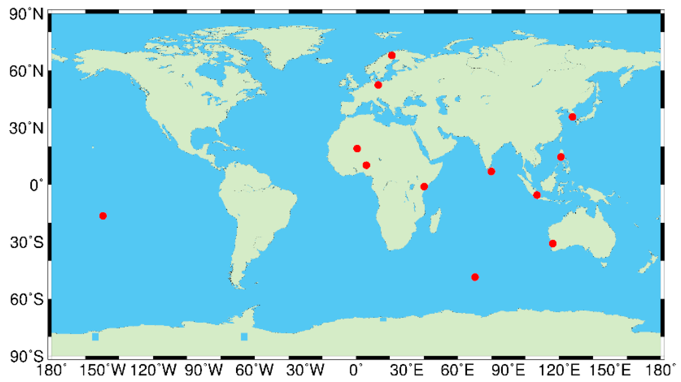
In this section, we mainly introduce the experimental protocol and data. To investigate the feasibility of IFB stochastic modeling on the performance of BDS-3, observation data sampled at 30 s on 1 January 2022 from the MGEX tracking network were selected. These stations are distributed around the world and equipped with receivers from three manufacturers, all of which can track B1I, B3I, B1C, B2a, and B2b five-frequency observations of BDS-3, as shown in Table 1. Figure 1 shows the geographical distribution of the selected stations with Multi-GNSS tracking capability.

Table 1.
The details of the GNSS receivers of the selected stations.
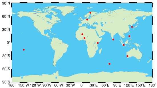
Figure 1.
Geographical distribution of the 12 global MGEX tracking stations.
3.2. Processing Strategy
The details of the data-processing strategy are given in Table 2. The precise orbit and clock products from Wuhan University (ftp://igs.gnsswhu.cn/pub/whu/phasebias/2022/, final products prefixed with WUM accessed on 1 January 2022). To reduce the influence of undetected pseudorange gross error and cycle slips on PPP, the detection, identification, and adaptation (DIA) quality-control method is applied [29,30]. When the standardized residual of the phase observation is greater than 5, the ambiguity of this satellite exceeds reset as a new parameter. Using DIA quality control in PPP software, we constructed the ω-test statistic assuming independent observations, and then the ω-test values were standardized residuals:
Table 2.
The data-processing strategy of BDS-3 UC-PPP for five-frequency observations.
For the carrier phase observation value, when the test quantity exceeds the threshold (set as 5 in this paper), we reset the ambiguity parameter. Since the BDS GEO satellite can only observe the signals of B1I and B3I frequencies, the observation data of GEO satellite are not used in this experiment. The pseudorange and phase standard deviation values of the BDS IGSO/MEO satellites are set to 0.3 m and 0.003 m, respectively.
In addition, the igs14_2188.atx (https://lists.igs.org/pipermail/igsmail/, accessed on 1 March 2022) file is used to correct the satellite and station antenna PCO/PCVs for BDS-3. When the PCO/PCV products of BDS-3 are used to eliminate the corresponding errors, it is recommended to use the method consistent with the IGS orbit determination. The position coordinates and clock are modeled as white noise in kinematic PPP modes. The IGS weekly solution is used as the true value of the station coordinates, with the positioning error the difference between the true value and the estimated coordinates. The and slant ionosphere delays are estimated as random walk noises with power density of and , respectively. The estimate of the float ambiguity is arc-constant until cycle slips.
The three schemes mentioned above are marked as IFB1 (white noise process), IFB2 (random walk process), and IFB3 (random constant process), respectively. The spectral density of IFB2 is calculated by the square of the inter-epoch variation divided by the sampling interval. The white noise model is used to estimate the inter-epoch variation of the receiver IFB time series in the 12 observed stations, with the station coordinates fixed to known accurate values.
4. Results and Discussion
Through the previous analysis, we conclude that the IFB is composed of pseudorange hardware delays for the baseline frequencies and non-baseline frequency. The comparison of IFB estimated by the three dynamic models is first presented. Subsequently, we analyze the different IFB modeling methods for these parameters in terms of observation residuals, zenith wet delay, ionosphere delay, and floating ambiguity. Finally, the observation data of globally distributed tracking stations are used to verify the impact of IFB stochastic modeling on the positioning performance of multi-frequency UC-PPP.
4.1. The Characteristics of Time Series for IFB
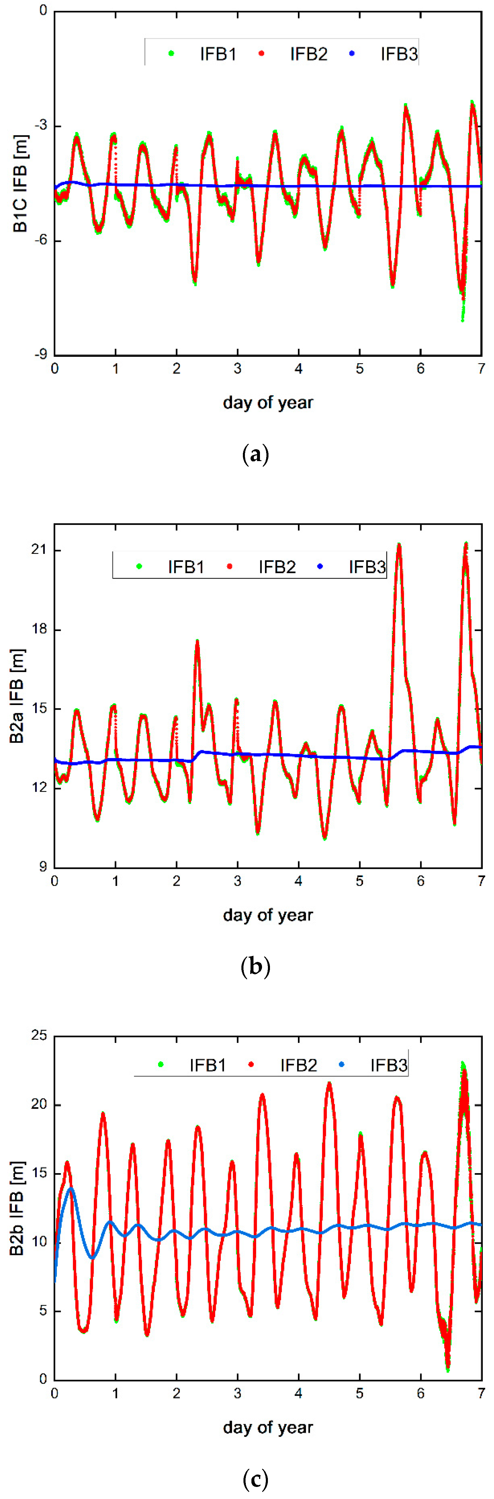
Before analyzing the influence of stochastic modeling for IFB on PPP, we first investigated the time-varying characteristics of IFB. Three methods of estimating IFB are white noise process, random walk process, and random constant. The one-week time series of the IFB station with different frequencies are shown in Figure 2. Figure 2a–c represents the IFB time series of the three frequency points B1C, B2a, and B2b, respectively. In general, the method of modeling with white noise can better estimate the inter-epoch variation of parameters. Therefore, we use the estimated IFB by the white noise model to analyze its temporal characteristics. To accurately estimate the IFB time series, the coordinates of the tracking station are fixed to known precise values with an accuracy of millimeters. Therefore, the actual estimated unknown parameters include receiver clock errors, zenith tropospheric wet delay parameters, and oblique paths. For the ionospheric delay parameters and ambiguity parameters, bidirectional filtering is used to eliminate the influence of the parameter convergence stage.
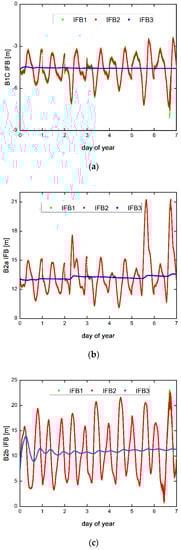
Figure 2.
The IFBs of B1C (a), B2a (b), and B2b (c) among different IFB handling schemes for station KRGG on day of year (DOY) 001 to 007 in 2022. IFB1, IFB2, and IFB3 represent three stochastic modeling methods of white noise, random walk, and time constant, respectively.
As shown in Figure 2, the IFBs of the three frequency points are not stable within one week. The receiver IFB of frequency observations B1C, B2a, and B2b has periodic changes in one week, and one period is a day. The variation range of IFB time series at different frequencies is dissimilar. The maximum frequency is B2b with a standard deviation of 5.139 m; the minimum is B1C with a standard deviation of 0.950 m; and the standard deviation of B2a is 1.964 m. Therefore, the method of estimating IFB as a time constant within one day cannot accurately eliminate the effect of IFB. The change in each frequency point in one week has obvious periodicity, but the inducement of this periodic change is still unclear and needs further study. The change period of the IFB at each frequency point is highly consistent, but the change amplitude is slightly different. The B1C and B2b frequency points have similar and larger change ranges, while the B2a frequency points have a smaller change range. The IFB time series estimated by the random walk model and the white noise model is relatively close, with the changes more severe at the peaks and troughs of the IFB series; for example, around 6 h, 12 h, 18 h, and 24 h, the difference between these two series is larger than other periods.
After analysis, we know that the IFB is unstable within one day and the variation range is several decimeters. There are significant differences between the IFB time series estimated by different stochastic modeling methods. In theory, these differences will affect the accuracy of other parameters of the filter, such as the user’s position, ionosphere, and troposphere. Therefore, we will analyze the influence of different stochastic modeling methods of IFB on the multi-frequency undifferenced and uncombined precise point positioning.
4.2. The Influence of IFB Stochastic Models on Observation Residuals
In this section, we mainly analyze the impact of three IFB stochastic modeling methods on the observation residuals. The distribution of the observation residuals can reflect the accuracy of functional models and stochastic models, and residuals also play an important role in the quality-control process. We first use the static solution mode to preprocess the observation data, eliminating those values containing pseudorange gross errors. Secondly, to ensure that the “clean” observation data participates in the processing, the residuals distribution of observations corresponding to three stochastic models is analyzed. Finally, the influence of three IFB stochastic modeling methods on gross error detection is analyzed to provide a reference point for quality control.
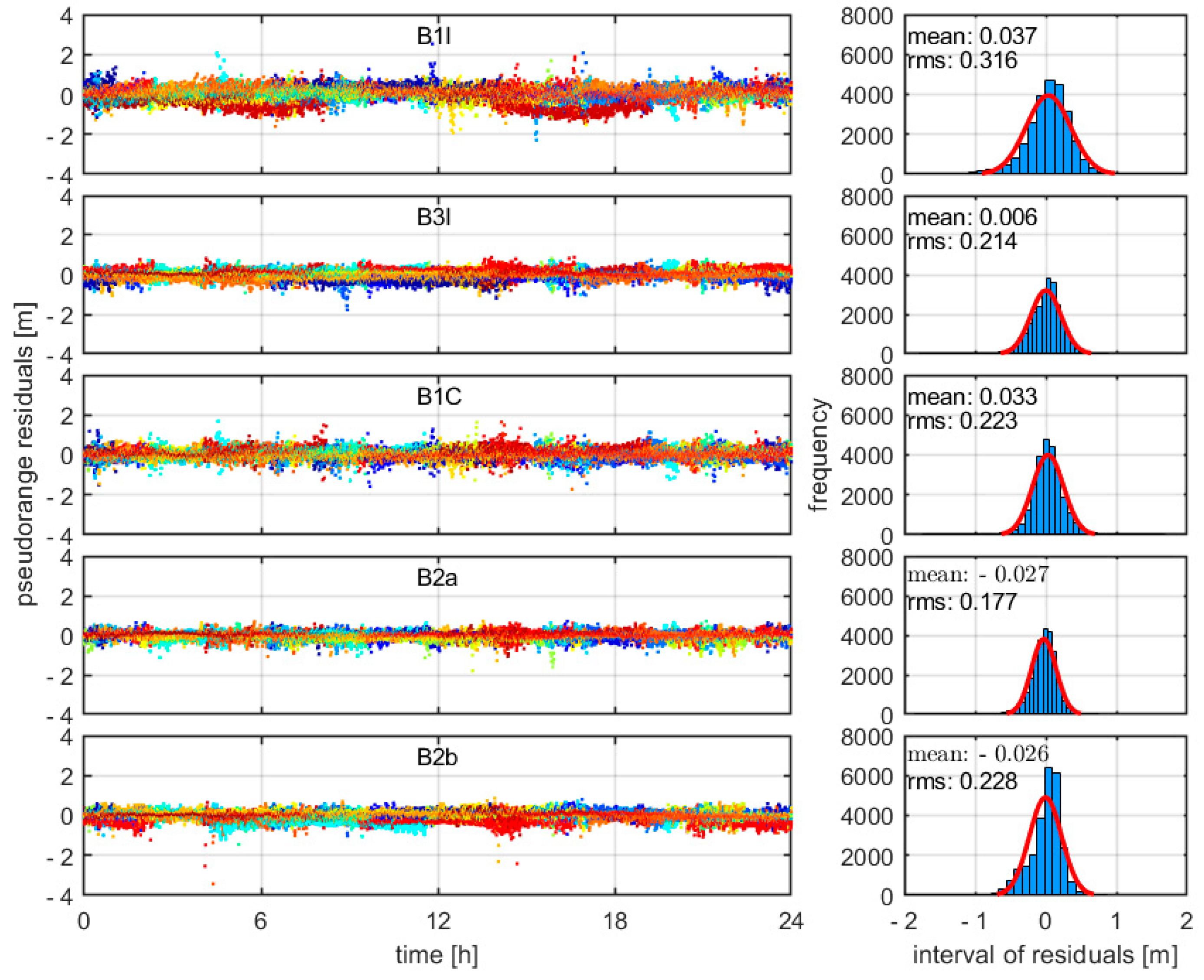
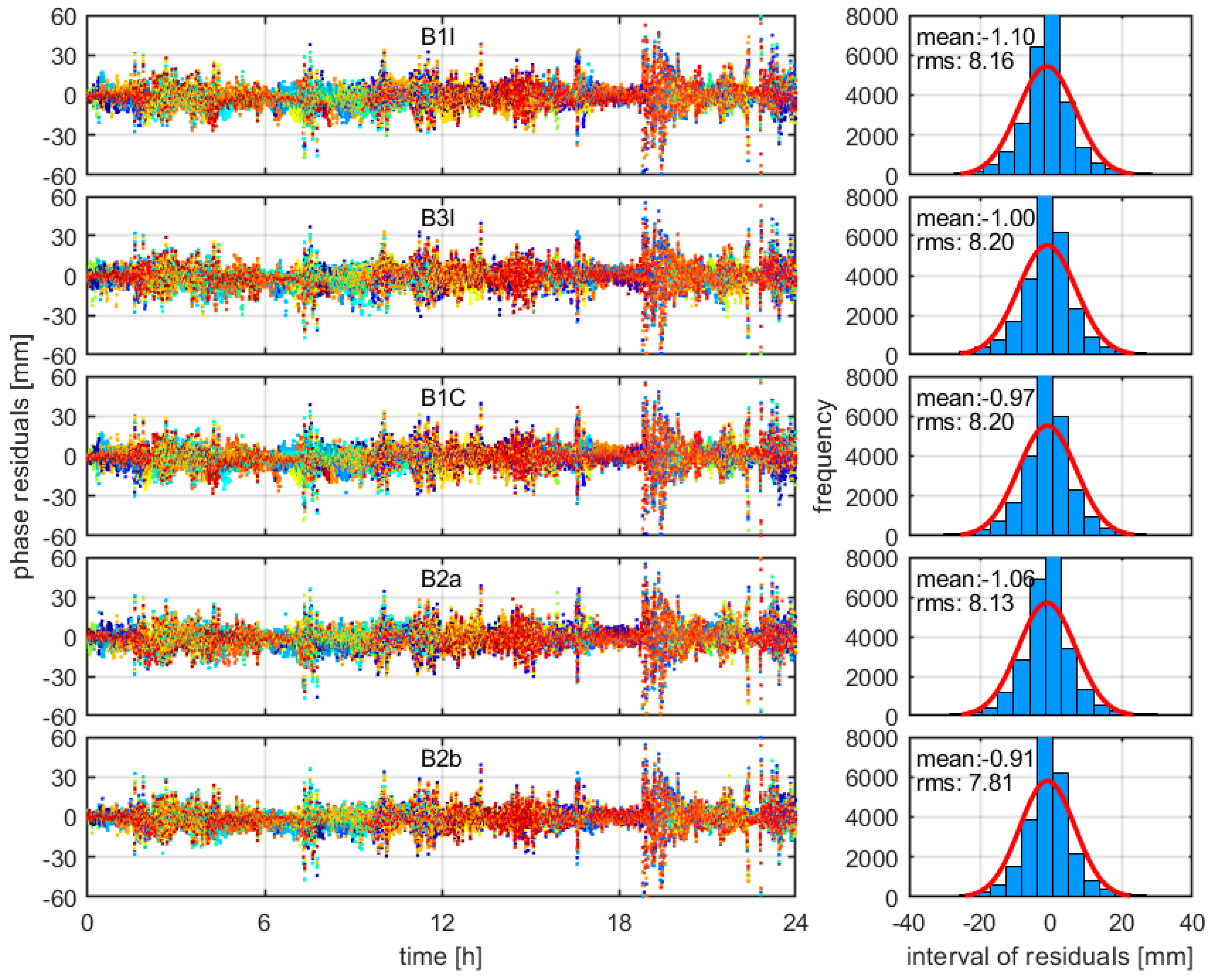
The distribution of the residuals approximating a zero-mean normal distribution indicates the superiority of the model in error correction accuracy. Taking the KRGG stations as an example, Figure 3 and Figure 4 show the pseudorange and phase residuals of the five-frequency UC-PPP kinematic model on DOY 001, 2022, where the left and right figures represent the observation residuals and the probability distribution of residuals, respectively. In the left figure, different satellites are represented by different colors. In the right figure, the red line represents the zero-mean probability distribution, indicating the completeness of the PPP model.
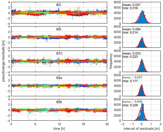
Figure 3.
The pseudorange residuals for BDS-3 UC-PPP of IFBs for stochastic modeling of random constant for station KRGG on DOY 001, 2022. The residuals of each satellite are represented with different colors. The right part of each subfigure shows the histogram of the residuals and the fitted normal density function (red line).
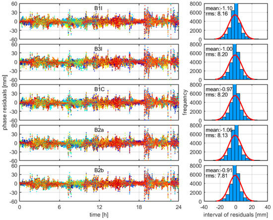
Figure 4.
The phase residuals for BDS-3 UC-PPP of IFBs for stochastic modeling of random constant for station KRGG on DOY 001, 2022. The residuals of each satellite are represented with different colors. The right part of each subfigure shows the histogram of the residuals and the fitted normal density function (red line).
Figure 3 and Table 3 show that for the baseline frequency, the mean and RMS differences on the pseudorange residuals of three IFB stochastic modeling methods are small, measuring only millimeters. For other frequencies, three IFB stochastic modeling methods can result in centimeter-level differences on pseudorange residuals. The mean and RMS of the pseudorange residuals are the same for the white noise and random walk models. The distributions of the pseudorange residuals between the white noise and random walk models and the time constant model are significantly different, with the mean differences being in centimeters, while the RMS differences are small. The mean value of the first two stochastic modeling methods is closer to 0 and the performance is better.
Table 3.
The means and RMS of the pseudorange residuals among different IFCB handling schemes.
As shown in Figure 4 and Table 4, the carrier phase residuals of three IFB stochastic modeling methods have small differences, with the mean difference less than 1 mm, while the RMS difference is the largest at 1.38 mm. The RMS of the carrier phase residual in the random walk model is the smallest, followed by the white noise model, with the time constant model the largest.
Table 4.
The means and RMS of the phase residuals among different IFCB handling schemes.
It can be seen that the IFB stochastic model can lead to large changes in the pseudorange residuals distribution of non-baseline frequencies, with a mean difference of several centimeters. The mean value of the pseudorange residual corresponding to the random walk model is the closest to 0, with the RMS smaller than other models. The IFB stochastic model has little influence on the distribution of the carrier phase residual, which is less than the millimeter level. In terms of the residuals distribution, the random walk model has better performance.
The residuals distribution of observations evaluates the accuracy of the model for statistical significance. The residuals are approximately closer to the normal distribution the more accurate the model is. Observation residuals also affect quality control. It can be seen from the previous analysis in this section that the IFB stochastic model mainly affects the pseudorange residual and has little effect on the carrier phase residual.
Although the contribution of pseudorange is much smaller than that of the carrier phase in the positioning process, the current quality-control methods are all based on standardized residuals, for instance, the DIA quality-control process and the IGG (Institute of Geodesy and Geophysics) [31,32] scheme. In these quality-control methods, the residual of the pseudorange has the same state as the residual of the carrier phase after variance normalization, so even a small gross error in the pseudorange may start the quality-control process.
The overall test is typically used for the detection of gross errors in the DIA quality-control method. The test statistic read as:
where denotes the post-test residuals, is the variance of observations, is the number of observations, and is the number of parameters to be estimated. With a critical level , if , the null hypothesis that there are no outliers is accepted; otherwise, the hypothesis that the outlier exists in the observations is accepted. Since we have gone through data preprocessing, gross errors are eliminated. Therefore, in theory, all statistical values satisfy . We chose the 95% confidence level and counted the false-alarm rate, with the false-alarm rates of 12 observation stations shown in Table 5.
Table 5.
False-alarm rate of overall test for three IFB stochastic modeling methods.
The false-alarm rates of 12 observation stations demonstrate that the time constant model has the highest false-alarm rate, and this phenomenon exists in most of the stations. The false-alarm rate of some sites is comparable to the time constant model when we use the white noise model. The false-alarm rate of the random walk model is the lowest among all stations. The mean false-alarm rates are shown in Table 5.
In general, the false-alarm rates corresponding to three IFB stochastic models are quite different. The time constant model has the highest false-alarm rate, followed by the white noise model, with the random walk model the smallest. This indicates that although the white noise model can accurately estimate the change in IFB, the larger process noise reduces the strength of the kinematic PPP positioning model and causes a higher false-alarm rate. The random walk model obtains a lower false-alarm rate, with a possible explanation for this being that the IFB value obtained based on the time-varying model could approximate the actual value. Another possibility for the reduced false-alarm rate is that the PPP positioning model has preserved intrinsic high strength.
4.3. The Influence of IFB Stochastic Models on ZWDs, Slant Ionospheric Delays, and Ambiguities
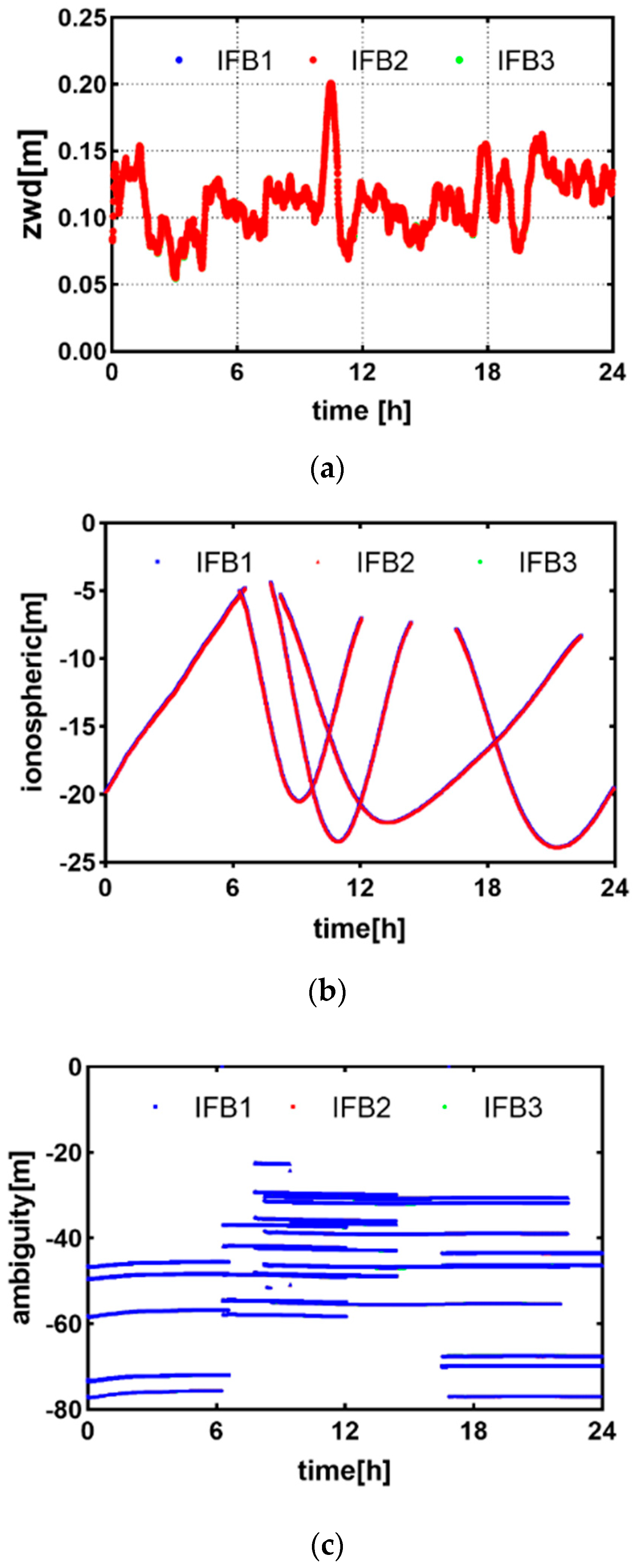
This section discusses the influence of the IFB stochastic model on zenith tropospheric delay, slant ionospheric delay, and floating ambiguity. Figure 5a shows the zenith wet delay at the KRGG station. The difference in the zenith wet delay calculated by three IFB stochastic models is extremely small, in the order of millimeters. Figure 5b is the ionospheric delay error of two MEO satellites, C19 and C20, and two IGSO satellites, C39 and C40. The ionospheric difference calculated by the three stochastic modeling methods is small and is millimeter-level. The floating ambiguities of the two MEO satellites, C19 and C20, and the two IGSO satellites, C39 and C40, are shown in Figure 5c; it demonstrates that the impact of three IFB modeling methods on the floating ambiguity is negligible. The IFB stochastic model has little influence on the troposphere, ionosphere, and ambiguity.
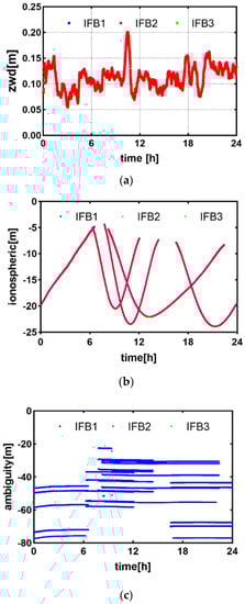
Figure 5.
The tropospheric ZWDs, slant ionospheric delays, and ambiguities of BDS-3 UC-PPP among different IFB handling schemes for station KRGG on DOY 001, 2022. Subfigures (a) is the tropospheric ZWDs of for station KRGG. Subfigures (b,c) are the slant ionospheric delays and float ambiguities of MEO satellites C19 and C20 and IGSO satellites C39 and C40, respectively.
4.4. The Influence of IFB Stochastic Models on PPP Performance
The performance of kinematic PPP was evaluated by convergence time and positioning accuracy, with 24 h observation data of each station applied. If the 3D positioning error of the current epoch and the following 20 epochs were less than the predefined threshold, we define this epoch as “convergence”. In this paper, we define the threshold as 1 dm. The positioning errors of UC-PPP for station KRGG on DOY 001, 2022, are presented in Figure 6.
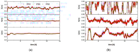
Figure 6.
The 3D positioning errors of UC-PPP for station KRGG on DOY 001, 2022. The E, N, and U represent the errors in positioning in the east, west, and south up directions of station KRGG, respectively. Subfigures (a,b) represent global positioning error and local positioning error.
It can be seen from Figure 6a that the E direction of the KRGG station takes a long time to converge, while the other two directions converge to higher accuracy in a very short time. Among three IFB stochastic models, the random walk model has the shortest convergence time, followed by the white noise model and then the time constant model. The kinematic PPP positioning accuracy of three IFB stochastic models has little difference. As shown in Figure 6b, after the parameters converge, there are differences in the positioning accuracy of three IFB stochastic models, but the overall difference is small. IFB mainly affects the pseudorange and has a greater impact on the convergence time. This section has a consistent conclusion with other scholars on the relationship between pseudorange accuracy and PPP convergence time.
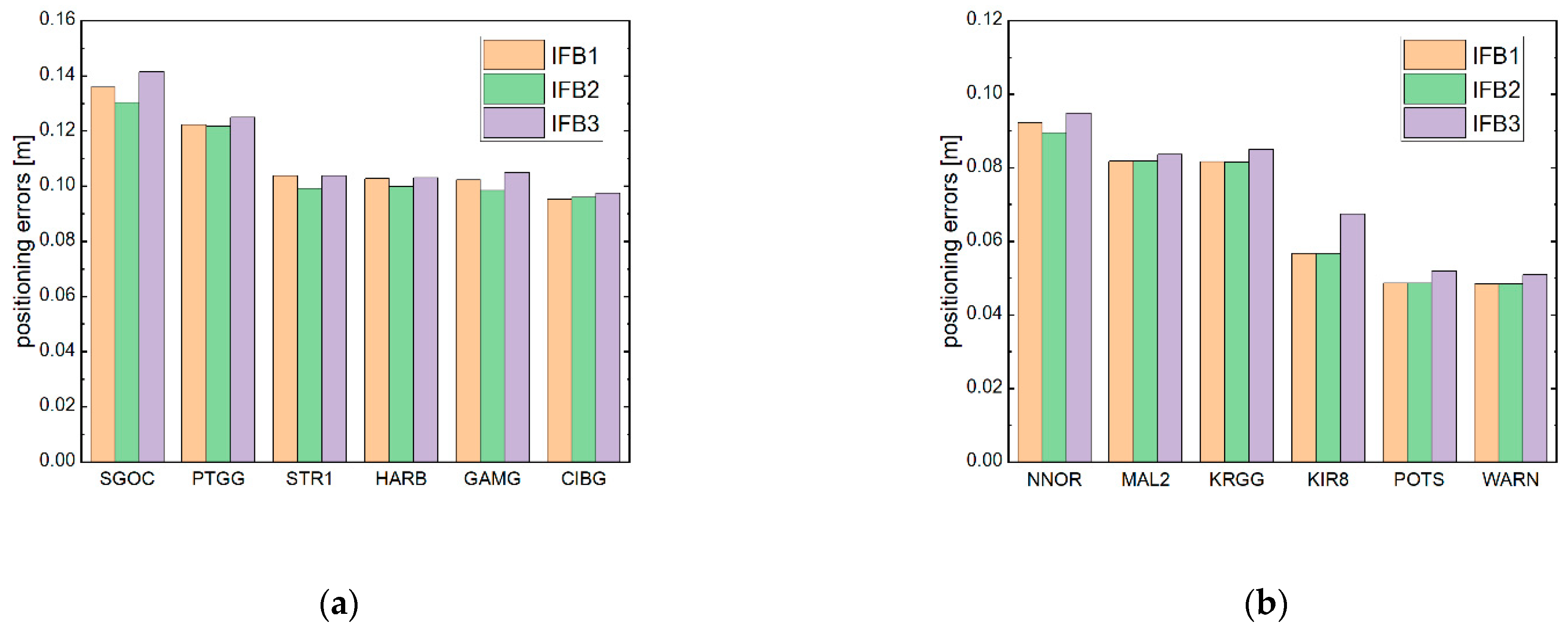
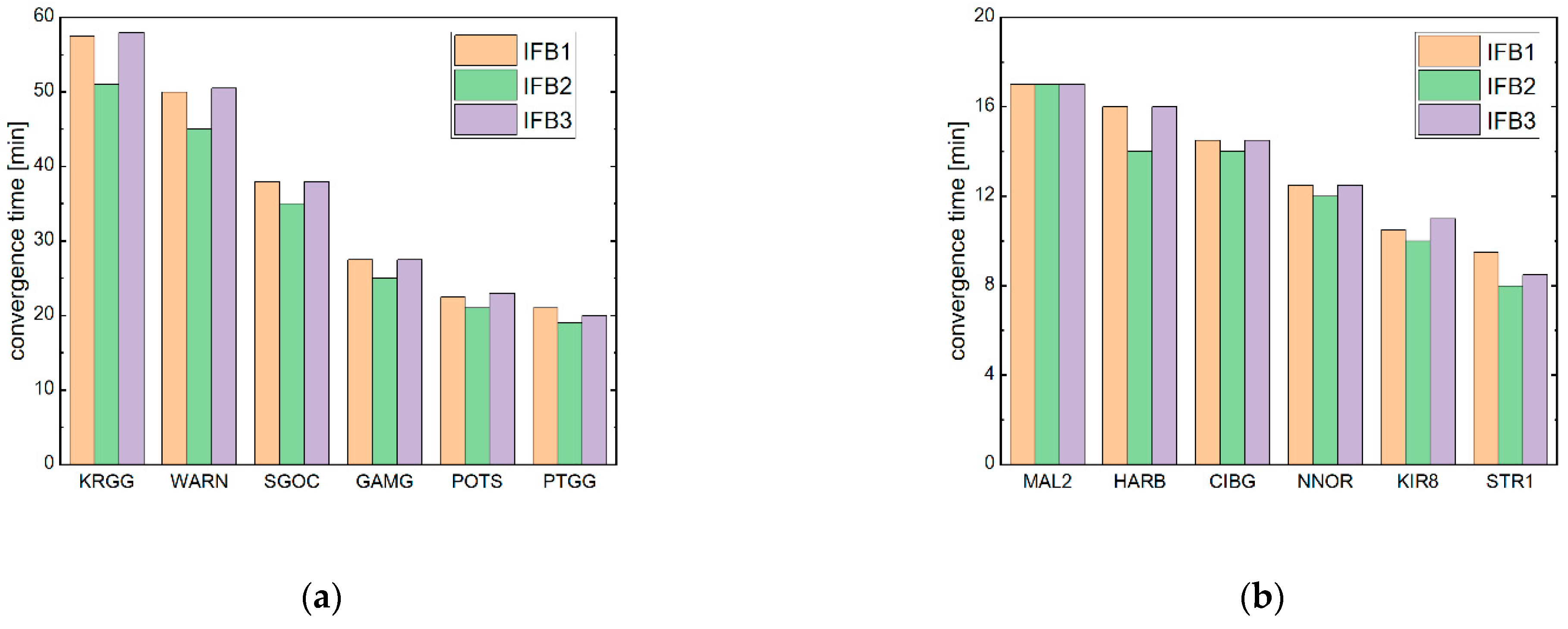
We conducted kinematic PPP positioning tests on the positioning accuracy and convergence time of 12 stations. Figure 7 and Table 6 summarize the obtained positioning accuracy, while Figure 8 and Table 7 illuminate the convergence time.
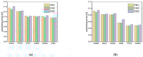
Figure 7.
The positioning errors of UC-PPP for different schemes. Subfigure (a) is used to represent the stations whose positioning accuracy is greater than 0.1 m, and subfigure (b) is for other stations.
Table 6.
The 3D positioning accuracy of UC-PPP for different schemes.
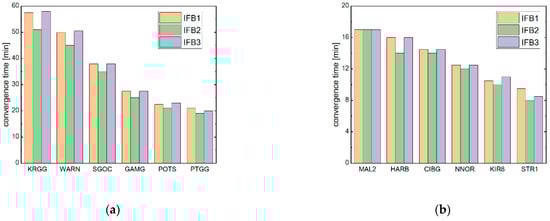
Figure 8.
The convergence time of UC PPP for different schemes. Subfigure (a) is used to represent the stations whose convergence time is greater than 20 min, and subfigure (b) is for other stations.
Table 7.
The convergence time of UC PPP.
We can see that there are differences in the positioning accuracy of the PPP data-processing schemes corresponding to three IFB stochastic models, but the overall difference is small. Among the three schemes, the random walk model has the highest positioning accuracy. The accuracy of the white noise model and the time constant model is basically the same. Although the white noise model has an advantage in the estimation accuracy of IFB, the larger process noise reduces the overall strength of the positioning model, resulting in no substantial improvement in the positioning accuracy. The time constant cannot accurately describe the time change of IFB, which leads to a decrease in the positioning accuracy in some periods, especially during the convergence period and when a large number of ambiguity parameters reconverge. The random walk model not only accurately describes the temporal variation of IFB, but also ensures the strength of the kinematic PPP positioning model with low process noise, so the positioning accuracy is the highest among the three models.
There are differences in the convergence times of the BDS-3 five-frequency uncombined PPP obtained by the three stochastic modeling schemes, with the data-processing scheme corresponding to the random walk model having the shortest convergence time. Compared with the white noise model, the random walk model shortens the convergence time by about 4~12%. The convergence times of the data-processing schemes corresponding to the white noise model and the time constant model are basically the same. At the STR1 station, the convergence time was longer in the white noise model compared with the time constant model. The reason for this phenomenon is that the number of available satellites in the observation data is low. The white noise model further reduces the strength of the kinematic PPP positioning model, resulting in a longer convergence time.
Therefore, when the solution involves enough satellites, the random walk model can slightly improve the positioning accuracy and shorten the convergence time by about 4~12%.
5. Conclusions
This paper mainly analyzes the impact of different IFB stochastic models on undifferenced and uncombined precise point positioning. We deduced that the IFB is mainly composed of the pseudorange hardware delay of the baseline frequency and pseudorange hardware delay of the corresponding frequency from the original observation equation, and analyzed the time-varying characteristics of the B1C, B2a, and B2b triple-frequency IFB by using the BDS-3 observation data. We evaluated the impact of three stochastic modeling methods on positioning performance. Using the random walk model to simulate the IFB can shorten the convergence time to a certain extent, reduce the false-alarm rate of the quality-control process, and improve the positioning accuracy. The random walk model is recommended to simulate the variation of IFB, which can not only overcome the disadvantage of the time constant model being unable to accurately describe the time-varying characteristics of the IFB, but also avoid reducing the strength of the kinematic PPP positioning model due to the large process noise of the white noise model.
Author Contributions
Conceptualization, Y.L. and W.Z.; design, Y.L. and W.Z.; experiments, D.Y.; analysis, D.Y.; writing—original draft preparation, D.Y.; writing—review and editing, S.B., S.G. and B.J.; discussion, S.B., S.G. and B.J.; PPP software, D.L. All authors have read and agreed to the published version of the manuscript.
Funding
This work was supported by the National Natural Science Foundation of China (no. 42174051, 41971416, 41874091), Graduate Innovation Foundation for Naval University of Engineering (DQCXJ2021004, DQCXJ2021005).
Data Availability Statement
The datasets analyzed in this study are managed by IGS.
Acknowledgments
All authors gratefully acknowledge IGS for providing the data, orbit, and clock products.
Conflicts of Interest
The authors declare no conflict of interest.
References
- Yang, Y.; Liu, L.; Li, J.; Yang, Y.; Zhang, T.; Mao, Y.; Sun, B.; Ren, X. Featured Services and Performance of BDS-3. Sci. Bull. 2021, 66, 2135–2143. [Google Scholar] [CrossRef]
- Duong, V.; Harima, K.; Choy, S.; Laurichesse, D.; Rizos, C. Assessing the Performance of Multi-Frequency GPS, Galileo and BeiDou PPP Ambiguity Resolution. J. Spat. Sci. 2020, 65, 61–78. [Google Scholar] [CrossRef]
- Guo, F. Modeling and Assessment of Triple-Frequency BDS Precise Point Positioning. J. Geod. 2016, 90, 1223–1235. [Google Scholar] [CrossRef]
- Cai, C.; Gao, Y. GLONASS-Based Precise Point Positioning and Performance Analysis. Adv. Space Res. 2013, 51, 514–524. [Google Scholar] [CrossRef]
- Montenbruck, O.; Steigenberger, P.; Prange, L.; Deng, Z.; Zhao, Q.; Perosanz, F.; Romero, I.; Noll, C.; Stürze, A.; Weber, G.; et al. The Multi-GNSS Experiment (MGEX) of the International GNSS Service (IGS)—Achievements, Prospects and Challenges. Adv. Space Res. 2017, 59, 1671–1697. [Google Scholar] [CrossRef]
- Guo, J.; Zhang, Q.; Li, G.; Zhang, K. Assessment of Multi-Frequency PPP Ambiguity Resolution Using Galileo and BeiDou-3 Signals. Remote Sens. 2021, 13, 4746. [Google Scholar] [CrossRef]
- Zhang, X.; Wu, M.; Liu, W.; Li, X.; Yu, S.; Lu, C.; Wickert, J. Initial Assessment of the COMPASS/BeiDou-3: New-Generation Navigation Signals. J. Geod. 2017, 91, 1225–1240. [Google Scholar] [CrossRef]
- Modeling and Assessment of Five-Frequency BDS Precise Point Positioning|SpringerLink. Available online: https://link.springer.com/article/10.1186/s43020-022-00069-z (accessed on 7 June 2022).
- Li, B.; Zhang, Z.; Miao, W.; Chen, G. Improved Precise Positioning with BDS-3 Quad-Frequency Signals. Satell. Navig. 2020, 1, 1–10. [Google Scholar] [CrossRef]
- Li, X.; Li, X.; Liu, G.; Yuan, Y.; Freeshah, M.; Zhang, K.; Zhou, F. BDS Multi-Frequency PPP Ambiguity Resolution with New B2a/B2b/B2a + b Signals and Legacy B1I/B3I Signals. J. Geod. 2020, 94, 1–15. [Google Scholar] [CrossRef]
- Li, H.; Zhou, X.; Wu, B. Fast Estimation and Analysis of the Inter-Frequency Clock Bias for Block IIF Satellites. GPS Solut. 2013, 17, 347–355. [Google Scholar] [CrossRef]
- Liu, Y.; Ye, S.; Song, W.; Lou, Y.; Chen, D. Integrating GPS and BDS to Shorten the Initialization Time for Ambiguity-Fixed PPP. GPS Solut. 2016, 21, 333–343. [Google Scholar] [CrossRef]
- Geng, J.; Meng, X.; Dodson, A.H.; Ge, M.; Teferle, F.N. Rapid Re-Convergences to Ambiguity-Fixed Solutions in Precise Point Positioning. J. Geod. 2010, 84, 705–714. [Google Scholar] [CrossRef] [Green Version]
- Cao, X.; Shen, F.; Ge, Y.; Liu, C.; Zhang, S. Inter-Frequency Code Bias Handling and Estimation for Multi-Frequency BeiDou-3/Galileo Uncombined Precise Point Positioning. Meas. Sci. Technol. 2022, 33, 015012. [Google Scholar] [CrossRef]
- Li, X.; Li, X.; Liu, G.; Xie, W.; Guo, F.; Yuan, Y.; Zhang, K.; Feng, G. The Phase and Code Biases of Galileo and BDS-3 BOC Signals: Effect on Ambiguity Resolution and Precise Positioning. J. Geod. 2020, 94, 9. [Google Scholar] [CrossRef]
- Deng, Y.; Guo, F.; Ren, X.; Ma, F.; Zhang, X. Estimation and Analysis of Multi-GNSS Observable-Specific Code Biases. GPS Solut. 2021, 25, 100. [Google Scholar] [CrossRef]
- Li, M.; Yuan, Y. Estimation and Analysis of the Observable-Specific Code Biases Estimated Using Multi-GNSS Observations and Global Ionospheric Maps. Remote Sens. 2021, 13, 3096. [Google Scholar] [CrossRef]
- Li, H.; Xiao, J.; Zhu, W. Investigation and Validation of the Time-Varying Characteristic for the GPS Differential Code Bias. Remote Sens. 2019, 11, 428. [Google Scholar] [CrossRef] [Green Version]
- Fan, L.; Shi, C.; Wang, C.; Guo, S.; Wang, Z.; Jing, G. Impact of Satellite Clock Offset on Differential Code Biases Estimation Using Undifferenced GPS Triple-Frequency Observations. GPS Solut. 2020, 24, 32. [Google Scholar] [CrossRef]
- Geng, J.; Chen, X.; Pan, Y.; Zhao, Q. A Modified Phase Clock/Bias Model to Improve PPP Ambiguity Resolution at Wuhan University. J. Geod. 2019, 93, 2053–2067. [Google Scholar] [CrossRef]
- Duan, B.; Hugentobler, U. Comparisons of CODE and CNES/CLS GPS Satellite Bias Products and Applications in Sentinel-3 Satellite Precise Orbit Determination. GPS Solut. 2021, 25, 128. [Google Scholar] [CrossRef]
- Zhou, F.; Dong, D.; Li, P.; Li, X.; Schuh, H. Influence of Stochastic Modeling for Inter-System Biases on Multi-GNSS Undifferenced and Uncombined Precise Point Positioning. GPS Solut. 2019, 23, 1–13. [Google Scholar] [CrossRef]
- Zhang, B. PPP-RTK Based on Undifferenced and Uncombined Observations: Theoretical and Practical Aspects. J. Geod. 2019, 93, 1011–1024. [Google Scholar] [CrossRef]
- Geng, J.; Guo, J. Beyond Three Frequencies: An Extendable Model for Single-Epoch Decimeter-Level Point Positioning by Exploiting Galileo and BeiDou-3 Signals. J. Geod. 2020, 94, 14. [Google Scholar] [CrossRef]
- Zhou, F.; Dong, D.; Ge, M.; Li, P.; Wickert, J.; Schuh, H. Simultaneous Estimation of GLONASS Pseudorange Inter-Frequency Biases in Precise Point Positioning Using Undifferenced and Uncombined Observations. GPS Solut. 2017, 22, 19. [Google Scholar] [CrossRef]
- Liu, G.; Guo, F.; Wang, J.; Du, M.; Qu, L. Triple-Frequency GPS Un-Differenced and Uncombined PPP Ambiguity Resolution Using Observable-Specific Satellite Signal Biases. Remote Sens. 2020, 12, 2310. [Google Scholar] [CrossRef]
- Schaer, S.; Villiger, A.; Arnold, D.; Dach, R.; Prange, L.; Jaggi, A. The CODE Ambiguity-Fixed Clock and Phase Bias Analysis Products: Generation, Properties, and Performance. J. Geod. 2021, 95, 81. [Google Scholar] [CrossRef]
- Mi, X.; Zhang, B.; Odolinski, R.; Yuan, Y. On the Temperature Sensitivity of Multi-GNSS Intra- and Inter-System Biases and the Impact on RTK Positioning. GPS Solut. 2020, 24, 112. [Google Scholar] [CrossRef]
- Yang, L.; Shen, Y.; Li, B.; Rizos, C. Simplified Algebraic Estimation for the Quality Control of DIA Estimator. J. Geod. 2021, 95, 1–15. [Google Scholar] [CrossRef]
- Teunissen, P. Distributional Theory for the DIA Method. J. Geod. 2018, 92, 59–80. [Google Scholar] [CrossRef]
- Yang, Y.; Song, L.; Xu, T. Robust Estimator for Correlated Observations Based on Bifactor Equivalent Weights. J. Geod. 2002, 76, 353–358. [Google Scholar] [CrossRef]
- Klein, I.; Matsuoka, M.T.; Guzatto, M.P.; de Souza, S.F.; Veronez, M. On Evaluation of Different Methods for Quality Control of Correlated Observations. Surv. Rev. 2015, 47, 28–35. [Google Scholar] [CrossRef] [Green Version]

Publisher’s Note: MDPI stays neutral with regard to jurisdictional claims in published maps and institutional affiliations. |
© 2022 by the authors. Licensee MDPI, Basel, Switzerland. This article is an open access article distributed under the terms and conditions of the Creative Commons Attribution (CC BY) license (https://creativecommons.org/licenses/by/4.0/).