Abstract
On 26 August 2020, a devastating flash flood struck Charikar city, Parwan province, Afghanistan, causing building damage and killing hundreds of people. Rapid identification and frequent mapping of the flood-affected area are essential for post-disaster support and rapid response. In this study, we used Google Earth Engine to evaluate the performance of automatic detection of flood-inundated areas by using the spectral index technique based on the relative difference in the Normalized Difference Vegetation Index (rdNDVI) between pre- and post-event Sentinel-2 images. We found that rdNDVI was effective in detecting the land cover change from a flash flood event in a semi-arid region in Afghanistan and in providing a reasonable inundation map. The result of the rdNDVI-based flood detection was compared and assessed by visual interpretation of changes in the satellite images. The overall accuracy obtained from the confusion matrix was 88%, and the kappa coefficient was 0.75, indicating that the methodology is recommendable for rapid assessment and mapping of future flash flood events. We also evaluated the NDVIs’ changes over the course of two years after the event to monitor the recovery process of the affected area. Finally, we performed a digital elevation model-based flow simulation to discuss the applicability of the simulation in identifying hazardous areas for future flood events.
Keywords:
flash flood; change detection; rdNDVI; Sentinel-2; flow simulation; Charikar; Afghanistan; Google Earth Engine 1. Introduction
Flash flooding is one of the most destructive and recurring natural hazards on the planet. Flash floods are typically generated by significant rainfall in dry and semi-arid areas. It causes catastrophic damage and threats to life, property, and cultural heritage. Floods affect more people than any other sort of weather-related disaster and are a leading cause of natural disaster fatalities worldwide [1]. It is caused by natural factors such as severe rainfall, the spilling of water onto dry ground in the floodplain, rapid snowmelt, and the failure of man-made infrastructure such as dams and levees. Floods have had significant impacts on the human economy as well, as indirect effects on economic growth and societal well-being. Floods disproportionately affect the poor and most vulnerable people [2].
Climate and morphology differ geographically and seasonally, which influences flash floods [3]. Depending on flow attenuation and sediment loading, the influence might vary within a watershed. To decrease the effects of flash floods, understanding hydrological dynamics in drainage basins is important [4]. Evaluations of flood consequences are feasible, essential, and smart alternatives to flood prevention [5,6,7,8]. Unfortunately, dryland hydrological measurements and observations are intermittent and insufficient to characterize these processes due to a lack of understanding and calibration of hydrological models. In most situations, especially in less-developed countries, these data are unavailable owing to a lack of meteorological stations [9]. Regional increases in hydrological problems are alarming, and more data is needed to model and assess the relationship between urbanization, hydrology, and land-use planning [10]. Due to the limited number of meteorological stations and the uncertainty of the data, conducting hydrological modelling in a dry area is technically impossible.
Remote sensing technology has been recognized as a convenient tool to widely identify, monitor, and evaluate areas affected by natural disasters, including flash floods, because land use and land cover change can be effectively identified. Flood monitoring by satellite images would rapidly provide extensive details of the affected area. Several approaches and methodologies based on pixel- and object-oriented methods can be used to detect water by using optical satellite data, including supervised and unsupervised classification methods, transformation of spectral channels, texture analysis, visual interpretation, single-channel thresholding, and channel ratio use. In the mentioned approaches, water indicators are extremely beneficial. Their implementation is contingent on the formulation of a threshold value that differentiates water pixels from those representing other forms of land cover.
Several approaches for extracting water bodies from remotely sensed data have been developed by researchers. McFreeters [11] proposed the Normalized Difference Water Index (NDWI) to detect water features from Landsat TM by using band 2 and band 4. Rogers et al. [12] introduced a new NDWI for extracting water from Landsat TM by utilizing bands 3 and 5. To extract surface water bodies from raw digital Landsat data, McFreeters [11] proposed a threshold value of zero, with all positive NDWI values categorized as water and negative values classed as non-water. This threshold, on the other hand, makes it impossible to distinguish between built-up surfaces and water pixels. As a result, Xu [13] developed the Modified Normalized Difference Water (MNDWI) by using Landsat TM bands 2 and 5. When compared to other indicators, the MNDWI indicator has a stronger ability to reduce disturbances generated by buildings, vegetation, and soils [13]. Feyisa et al. [14] developed the Automated Water Extraction Index (AWEI) to increase the accuracy of water extraction in locations containing shadows and dark surfaces. The MNDWI has been used to create a simple Enhanced Water Index (EWI) by [15]. Surface water can be identified from background information such as deserts, soil, and vegetation. For the extraction of surface water from Landsat data, Rokni et al. [16] examined the characteristics of NDWI, MNDWI, AWEI, and the Normalized Difference Moisture Index (NDMI) in applying a novel surface water change detection process based on the principal components of multi-temporal NDWI. Surface water was retrieved from the indices by using a trial-and-error thresholding methodology. The overall accuracy and kappa coefficient were used to examine the efficacy of each water body extraction procedure, and NDWI was found to outperform other measures. These indices have also been used in a multitude of scenarios, such as surface water mapping [14,17], land use, and land cover change assessments [18], and ecological research [19]. On the other hand, numerous researchers have utilized the Normalized Difference Vegetation Index (NDVI) to detect land cover change because the NDVI shows positive values for vegetation, values close to zero for bare soil, and negative values for water [20,21,22]. Many studies show that AWEI and MNDWI achieved better results and more stable thresholds than the NDVI [23].
Modern satellites are better than traditional techniques for monitoring surface water, but downloading and processing vast study areas or long-term data is time-consuming. Most classic approaches are not straightforward, making them technically challenging to employ because of preprocessing [24]. We used the Google Earth Engine (GEE), a planetary-scale platform for earth science data and analysis developed by Google, to apply the spectral index technique developed in [25]. The GEE has enabled the development of global-scale products, tools, and services by using temporal earth observation data such as Sentinel-2. The GEE platform provides a fast-forward solution for these kinds of big data problems. The GEE has been used to conduct various global and regional scale studies, including regional land cover mapping [26], surface water mapping [27], accessing food security situations [28], settlement and population mapping [29], and other applications [30]. Hazard Mapper is an open-access application developed in the GEE [25] and has been used in many case studies and in different countries to delineate different kinds of natural hazards, but it has never been used for floods or flash floods.
Although the model’s original developer [25] never used it to estimate floods in non-vegetated environments such as high altitudes or semi-arid to arid regions, we are looking into it to see if it can be used to locate flood-inundated areas in non-vegetated, data-scarce regions such as Afghanistan. On 26 August 2020, the city of Charikar in Afghanistan was devastated by a flash flood, which caused significant damage to the residential sector and claimed the lives of hundreds of people. Nevertheless, the affected area has not been as scientifically investigated as other parts of the country due to safety and economic concerns. As a consequence of this, the actual location of the areas that were swamped by the flood, in addition to the extent of the flood damage region, is unknown to this day. There have been several research approaches developed in the field of remote sensing with almost all of them concentrating on the detection of floods in areas where there is accumulated water. On the other hand, there is no study that has been conducted up to this point that discusses the practicability of approaches for detecting flash flood-inundated areas in regions that do not have standing water. Most of the methods mentioned are frequently used by the researchers for extraction of water bodies such as lakes, canals, waterways, ponds, and so on. They never used methods such as the spectral index technique in flash flood situations when there was no standing water.
Thus, to fill the gap, this study investigates the utilization of freely available optical satellite data to evaluate flood-affected areas in Charikar to some extent, contributing to the remote sensing community and disaster management team for the identification and evaluation of damaged areas with better precision. This study intends to employ remote sensing and GEE to automatically detect flash flood-inundated areas quickly after the incident by using a change detection method based on pre- and post-event NDVIs in Sentinel-2 satellite images. Moreover, it is also the goal to estimate the area of flash flood to understand the magnitude of the flood and contribute to the planning for post-disaster activities. We also evaluate and compare the detected inundation area’s accuracy with flood maps derived from visual image interpretations and government reports. Furthermore, we use the time series to measure changes in NDVIs two years after the event date to follow the recovery process in the affected area. We also use a digital elevation model (DEM) to examine flow path assessment of gravitational hazards at a regional scale [31] in order to assess the feasibility of the simulation technique for finding and predicting vulnerable regions in future flood occurrences. In addition, feasible mitigating strategies have been recommended for any potential future incidents.
2. The Charikar Flash Flood and Dataset
2.1. Study Area
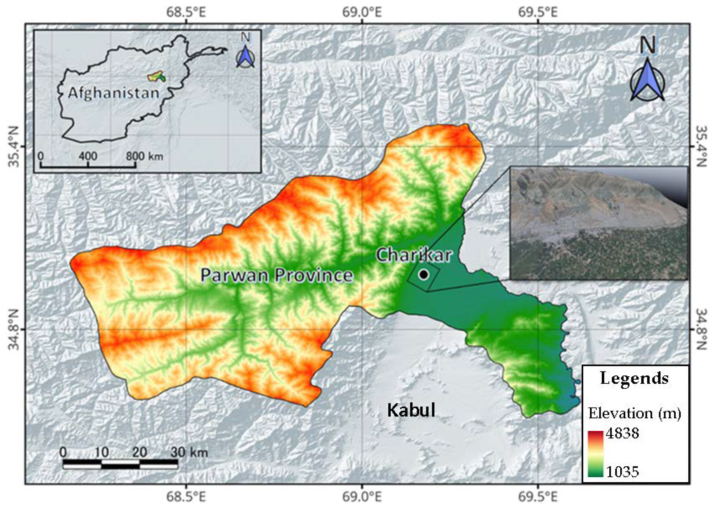
The study area is located in Afghanistan between latitudes 35°01′9.3″W and longitude 69°09′55.67″N, which includes parts of the capital of the Parwan province (Figure 1). The city lies on the Afghanistan Ring Road, 69 km from Kabul along the route to the northern provinces. It connects Kabul and the western parts of Afghanistan to northern parts of Afghanistan such as Mazar-i-Sharif, Kunduz, and Puli Khumri. Despite the proximity to Kabul, slightly more than half of the land is not built up.
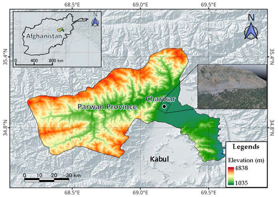
Figure 1.
Topographical map of the study area showing how Charikar city is surrounded by high mountains of Hindu Kush which the elevation is between 1000–4000 m.
The study area encompasses the central city of Charikar, as depicted by the rectangle in Figure 1, which covers 30,500 hectares and was devastated by flooding. The Ghorband river flows through Parwan province. It is a tributary of the Panjshir river, then a sub-tributary of the Indus River, and then the Kabul River. The Ghorband runs entirely in Parwan province, where it gave its name to the Ghorband district. It is born in the eastern Sheybar pass (which connects the provinces of Parwan and Bamyan, or watersheds of the Ghorband and Kunduz Rivers and passes in an eastbound direction, which it maintains throughout most of its course. It runs along the south and the imposing central range of the Hindu Kush, receiving meltwater in the Sheybar pass area of Salang. It flows from here through a long valley between the Hindu Kush mountains in the north and Koh-i-Baba in the south. It then connects to the Panjshir on its right bank, some 10 km east of Charikar. It runs through the Sheikh Ali, Shinwari, Ghorband, and Surkh Parsa districts.
Parwan is situated at a high elevation of 1800 m (5900 feet) above sea level. Winter is chilly, with an average temperature of −1 °C in January, freezing nights most of the time, and a probable high of −20/−25 °C; snowfalls are very common and sometimes substantial. Summer days are hot, occasionally blistering, and nights are normally cool. Precipitation in Charikar is rather low, averaging 300 mm per year. Spring is the wettest season. It rarely rains in the summer and the average summer high and low temperature fluctuate between 32 and 20 degrees respectively. Even in winter, the sun shines regularly in Charikar, and it shines frequently in summer.
2.2. The Flash Flood in Charikar
Afghanistan is a landlocked country with an arid to semi-arid climate vulnerable to a variety of hazards, including earthquakes, flooding, drought, avalanches, and man-made calamities [32,33]. A devastating flash flood occurred near the residential areas in Charikar city, Parwan province, Afghanistan on 26 August 2020, killing over 100 people. Most of the victims were children and women. More than 150 people were injured [34]. In the flash flood event, more than 17,000 people were affected, and nearly 2000 homes were destroyed [35]. The midnight floods surprised locals who were asleep. According to local witnesses, first a roar was heard and then a flood arrived at their houses [36]. Even police soldiers attempted air shooting to wake people, but unfortunately, most of the people did not notice. Rescue teams, locals and social groups were searching for the bodies of the victims. However, many people were missing. Based on a report [37], a person was missing nine members of his family. The substandard mud houses on the mountainside near the Opyan village (Figure 2) and some other areas around Charikar turned into rubble after the flood, as shown in Figure 3.

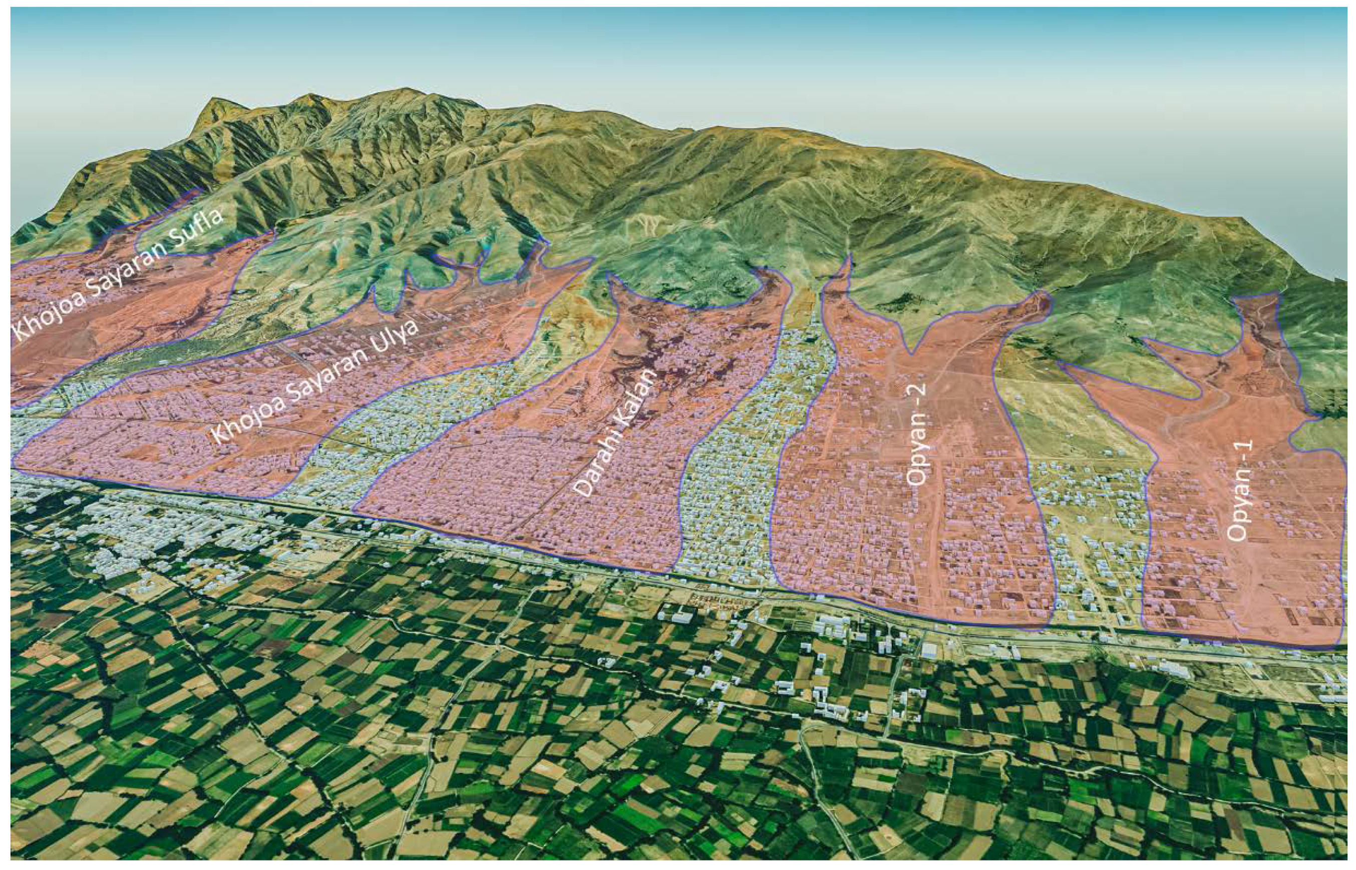
Figure 2.
Compounds in Charikar city are at risk of flooding due to a lack of regular urban planning. The flood path information is collected from the Surface Water Resources Department of Afghanistan.

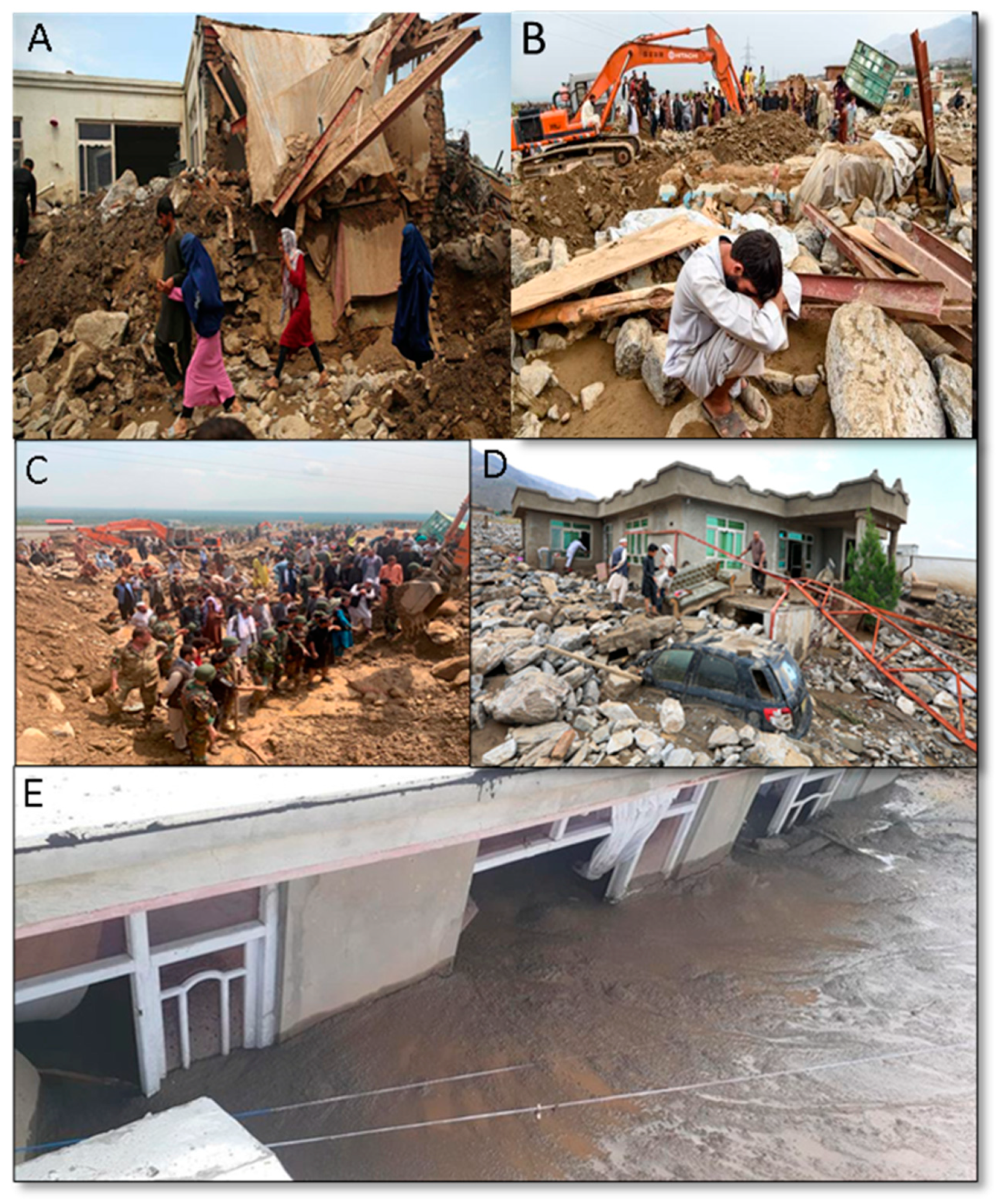
Figure 3.
The affected area in Charikar: (A) group of people walk near damaged houses in Charikar, Parwan province, on Wednesday, 26 August 2020. The image is reprinted/adapted with permission from Ref. [38], which can be accessed through Fox News. (B) A man reacts near to his ruined home as rescuers search for victims in Sayrah-e-Hopiyan, Charikar, Parwan province, on August 26, 2020, following a flash flood, photograph is reprinted/adapted with permission from Ref. [39]. (C) Villagers and soldiers search for victims in a mudslide caused by a flash flood at Sayrah-e-Opiyan in Charikar (Photo is reprinted/adapted with permission from Ref. [40]). (D) A flash flood brought debris and boulders into the house, covered the car, and injured and killed people. (Photo is reprinted/adapted with permission from Ref. [41]). (E) A general view of a building in Charikar, Afghanistan, covered in flooded debris from flooding on 26 August 2020, Reprinted/adapted with permission from Ref. [36].
This horrific occurrence, combined with the ongoing conflict and the COVID-19 outbreak, exacerbated the healthcare system’s reliance on foreign aid for even the most basic services. The city of Charikar is situated in a location where a variety of flood channels and valleys directly threaten the city’s residents. Due to population pressures, land scarcity, and improper land development, the majority of people in Afghanistan now live in hilly, flood-prone areas like Charikar, which will almost certainly result in an increase in flood-related building damage. As can be seen in Figure 2, areas that are prone to flooding, are represented by red outlines. Each red region has hundreds of residential buildings that are in danger of flooding at any given time, which puts the lives of the people living there at danger. Government regulation and regular urban planning have been neglected in the construction of new cities and buildings. The irregular and arbitrary land sales by landlords and local bullies, as well as the absence of floods in recent years in Charikar, have misled people to assume that it is safe to buy and construct houses in these hazardous places. Building and construction were expanding at a rate that had never been witnessed before the devastating flash flood. This ruined the lives of individuals and the economy.
2.3. Data Sets
Sentinel-2 satellite imagery is a constellation of two earth observation satellites, developed by the European Space Agency (ESA) and the European Commission’s ambitious Copernicus Program, consists of two identical satellites: Sentinel-2A, launched on 23 June 2015, and Sentinel-2B, launched on 7 March 2017, available in various processed formats [42]. The so-called multispectral instrument (MSI) products go through several rounds of processing before reaching a level that is usable. Level-0, Level-1A, Level-1B, Level-1C, and Level-2 are the primary stages. Users cannot access Level-0 and Level-1A, which are stored in the instrument source packet (ISP) format, which is a compressed raw picture data format. Level-1B has radiometrically corrected imagery with TOA radiance, which is built up of granules of 25 by 23 km in length. Level-1C has been formed in 100 × 100 km tiles in an orthorectified format in the UTM/WGS 84 projection [42]. The Sentinel-2 Toolbox can process Level 2A products from Level-1C products. The most commonly used products in land cover/use mapping are Level-1C and Level-2A. As part of the European Commission’s and European Space Agency’s free, complete, and open data policy, this dataset is freely distributed to the public domain. Since its introduction, Sentinel-2 data has been used in a variety of earth and atmospheric science research investigations, and is perfect for agriculture, forestry, and other land management applications [43,44,45,46], flood mapping [47,48,49], wetland monitoring [50], and agricultural operations [51,52]. The radiometric and geometric quality of Sentinel-2 data is technically superior to data acquired by other low spatial resolution data, such as Landsat data. For the purpose of this study, we utilized Sentinel-2 imagery acquired between the periods of 5 June 2020 and 23 October 2020. Table 1 presents an overview of the key features of the images used in this study. The Sentinel-2 has a 10-day return period at the equator and a five-day revisit time at mid-latitudes, as well as a spatial resolution of 10 m, which contributes to its dominance. Although they have the disadvantage of being affected by cloudiness, optical imaging satellites would be preferred for flood studies since the surface conditions of the affected areas are easily confirmed from the images compared to radar satellites data.

Table 1.
The distinguishing characteristics of the satellite imagery used in this study, as well as their observation conditions.
3. Methodology
The current study’s overall procedure is depicted in a flow chart in Figure 4. The NDVI, MNDWI, and NDMI indices and their correlations were discussed in Section 3.1, relative difference in NDVI (rdNDVI) and its formulation and procedures are discussed in Section 3.2, the histogram-based segmentation is discussed in Section 3.3, accuracy assessment by using the confusion matrix is discussed in Section 3.4, and prediction of probable future flood inundation by using Flow-R is evaluated in Section 3.5.
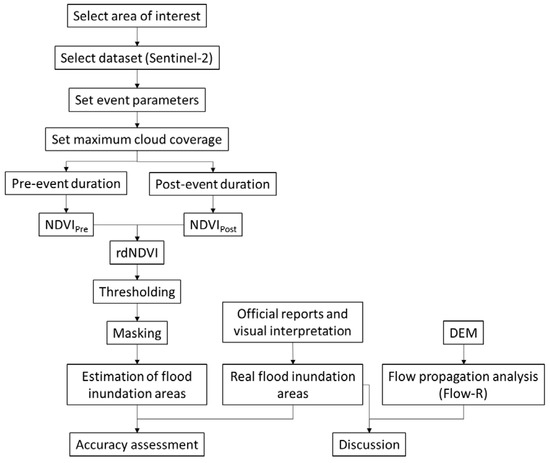
Figure 4.
Flowchart of the methodology used in this study.
3.1. NDVI and Spectral Water Indices
We did not investigate the extraction of water bodies in the affected area because there was no standing water after the incident. However, we used NDVI to assess and identify the inundated region because there are many indices established by researchers for the identification of flooded areas. To assess the performance of other indices in the impacted area, we intend to examine their applicability in the affected area shortly. To extract water bodies from remotely sensed data, several spectral water indices have been established, mainly by computing the normalized difference between two image bands and then applying an appropriate threshold to classify the outputs into two groups (water and non-water features). The MNDWI and NDMI indices are utilized by most researchers for the extraction of water bodies such as lakes, rivers, ponds, etc. The current study’s purpose is to use rdNDVI to delineate the inundated area following a flash flood where there are no leftover water bodies. Then we calculate and illustrate a correlation between NDVI and three spectral water indices to observe the output of each single index for detecting changes caused to the study area by the flash flood.
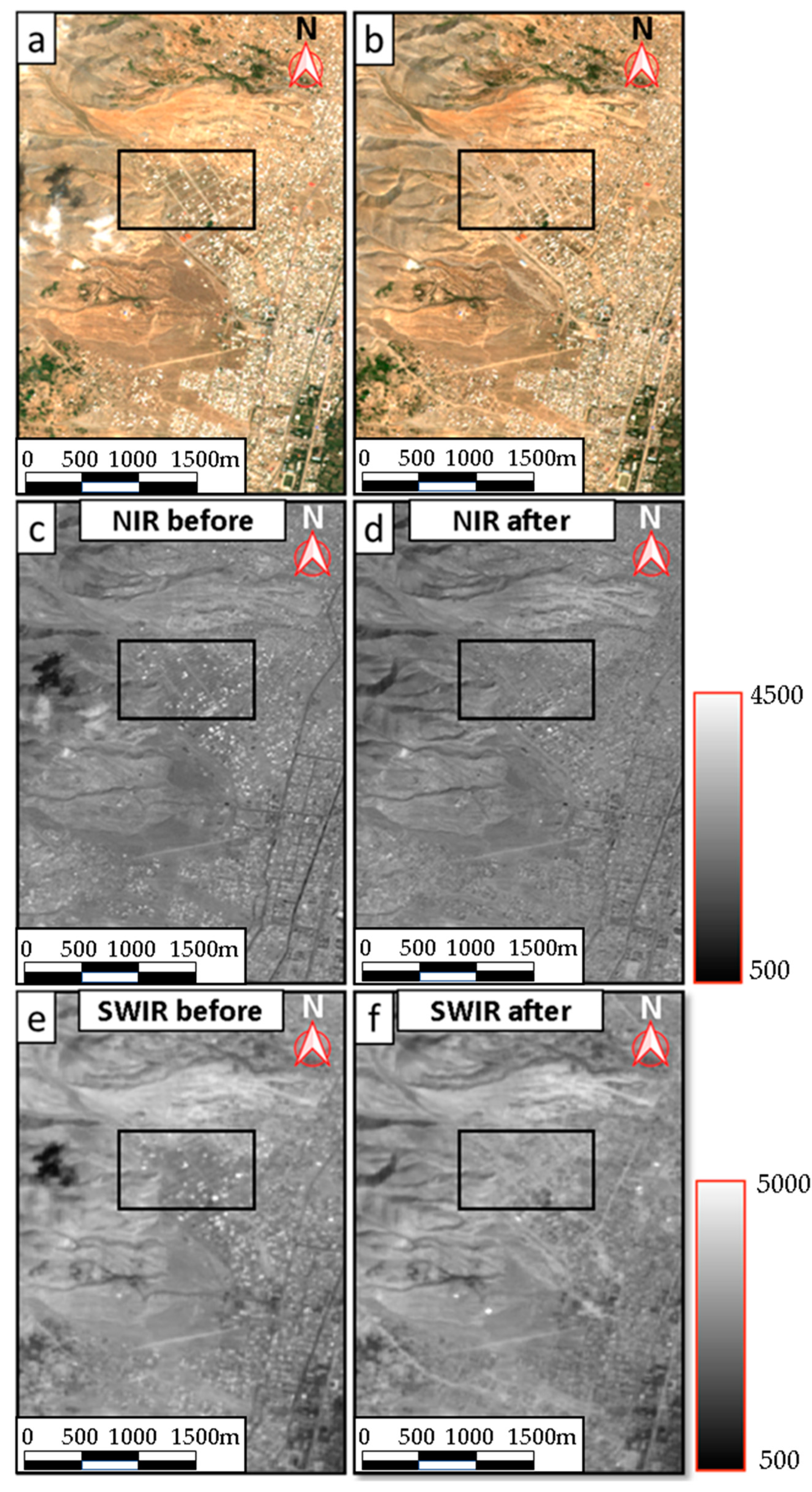
Figure 5a,b depicts the true color Sentinel-2 images observed before the flash flood on 24 August and after the flash flood on 13 September. If we examine those rectangular areas in Figure 5 we can clearly notice a trail of the inundated area that remains due mainly to the flood occurrence. The color of the soil in the affected area changed as a result of increased soil moisture after the flash flood. As shown in Figure 5c–f, the reflectance of such darkened wet soil is significantly low in infrared bands such as near infrared (NIR) and short wavelength infrared (SWIR). This means that spectral indices using NIR and/or SWIR would be effective to detect the flood-inundated areas.

Figure 5.
Observation of changes in the study area by using pre- and post-event Sentinel-2 satellite images. (a) True-color images acquired on 24 August 2020. (b) True-color image acquired on 13 September 2020. (c) NIR band acquired on 24 August 2020. (d) NIR band acquired on 13 September 2020. (e) SWIR band acquired on 24 August 2020. (f) SWIR band acquired on 13 September 2020. Rectangular area is selected on those areas to analyses the NDVI time series.
3.1.1. Normalized Difference Vegetation Index (NDVI)
The NDVI index uses reflected light in the visible and near-infrared bands to detect and quantify the presence of live green vegetation. Simply put, NDVI is a metric that may be used to classify land cover in remote sensing areas and can measure the density and health of vegetation in each pixel. The first formal report of the NDVI was in [53]. The NDVI is expressed by Equation (1),
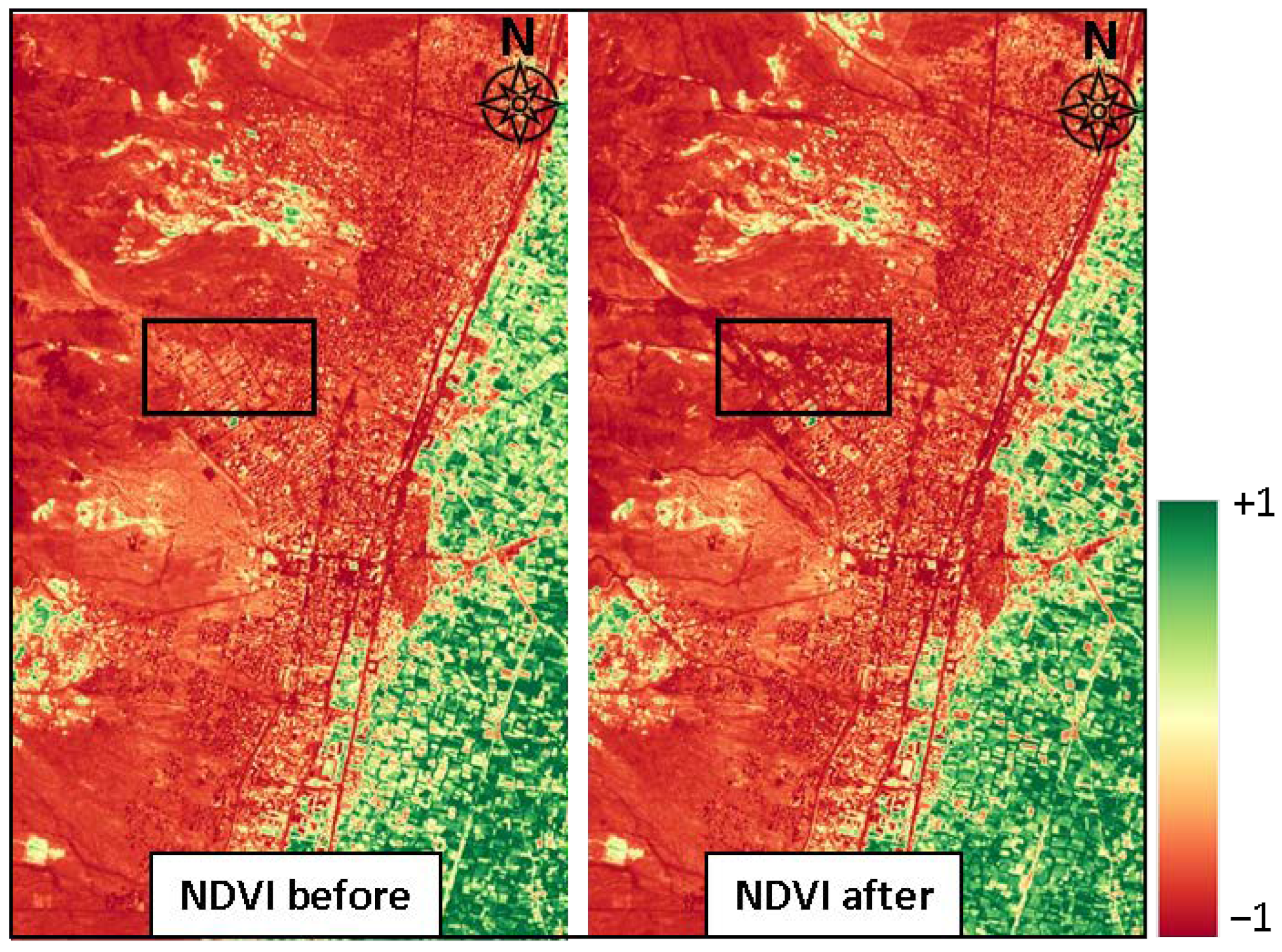
where NIR is the near-infrared band and red is the visible red band. This index ranges from −1.0 to 1.0, essentially depicting green, with negative values originating from clouds, water, and snow, and values close to zero originating from rocks and bare soil. The NDVI function has very low values (0.1 or below) that correlate to vacant expanses of rocks, sand, or snow. Medium values (0.2 to 0.3) show shrubs and meadows, whereas large values (0.6 to 0.8) show temperate and tropical forests. In Figure 6, we showed the estimated image of the NDVI index to see how the area hit by the flash flood had changed.

Figure 6.
Observation of changes in the study area using pre- and post-event NDVIs.
3.1.2. Normalized Difference Water Index (NDWI)
The normalized difference water index (NDWI) was developed by [11] for detecting surface water in wetland regions and surface water measurement and is defined as
where, for Sentinel-2, green and NIR are the reflectance of green (band 3) and NIR (band 8), respectively. The NDWI value ranges from −1 to 1. McFeeters [11] determined the threshold value as zero. That is to say, if NDWI is greater than zero, the type of cover is water; alternatively, if NDWI is less than zero, the type of cover is not water. According to the previous study [13], NDWI was unable to entirely differentiate built-up features from water features. Because the NIR reflectance was lower than the green reflectance, NDWI displayed positive values in built-up features that were comparable to water. Therefore, Xu [13] proposed the modified NDWI (MNDWI), which substituted the SWIR band (Landsat TM band 5) for the NIR band in McFeeters’ NDWI Equation (3):
where, for Sentinel-2, SWIR is the reflectance of short-wave infrared bands (Band 11). Equation (3) is used to enhance open-water features that are dominated by built-up areas. Noise from built-up land, vegetation, and soil is reduced considerably. We visually presented the estimated image of the MNDWI index in Figure 7. This allowed us to see the changes that had occurred in the area that had been inundated by the flash flood.
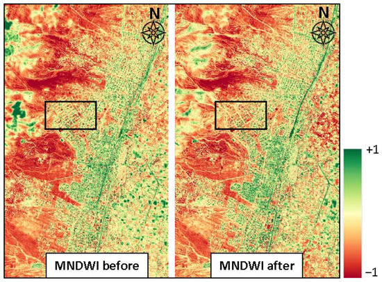
Figure 7.
Observation of changes in the study area using pre- and post-event MNDWIs.
3.1.3. Normalized Difference Moisture Index (NDMI)
The Normalized Difference Moisture Index (NDMI) was initially utilized by [54,55] to extract moisture content from biomass and vegetation. For Sentinel-2, the normalized difference moisture index (NDMI) is derived as a ratio between the NIR (band 8) and the SWIR (band 11) by using Equation (4),
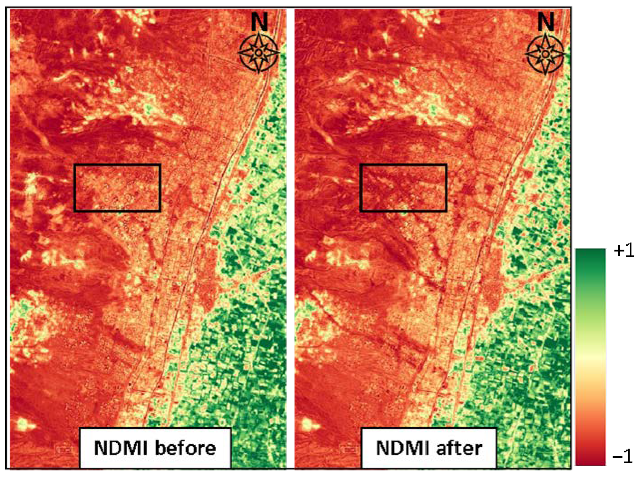
Like most indices, the NDMI value ranges between −1 and 1. Negative numbers approaching −1 indicate water stress, whereas higher values correspond to larger quantities of water. NDMI can detect water stress in early stages, before it becomes a serious problem. Furthermore, employing NDMI to monitor irrigation, particularly in locations where crops require more water than nature can provide, aids crop growth tremendously. In order to determine whether or not it is possible to observe the changes in the study area as a result of the impact of the flash flood by using NDMI, we illustrate the NDMI images in the study area in Figure 8. Initially, we assess the performance of NDVI, MNDWI, and NDMI in the inundated area and then show the correlation between the mentioned indices with NDVI.

Figure 8.
Observation of changes in the study area using pre- and post-event NDMIs.
We visually presented the estimated images of the indices in Figure 6, Figure 7 and Figure 8 to see the applicability of the index in detecting the changes in the flash flood-inundated area. To examine how the images would alter after the flood, we specified a completely identical color table ranging from (−1 to +1) for all of the estimated indices. As can be observed in Figure 6, the color in the rectangle area of the NDVI-post event shifted to dark red (+1), although in the same area, we noticed some changes in the MNDWI post-event (Figure 7), but it is not as pronounced as the NDVI. Additionally, the NDMI, in the selected rectangular area, depicts the changes as a result of the flood in a more pronounced manner (Figure 9), compared to the MNDWI (Figure 8). Particularly in the NDMI-after image, vast areas at the tops of the hills (surrounding the rectangular areas), are altered to darker colors (+1), indicating an overestimation of the inundation area.
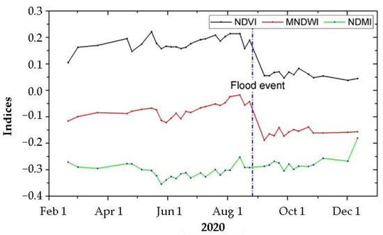
Figure 9.
Time series of the NDVI, MNDWI, and NDMI over the course of one year in affected area. The blue dotted line indicates the date of the flash flood in Charikar.
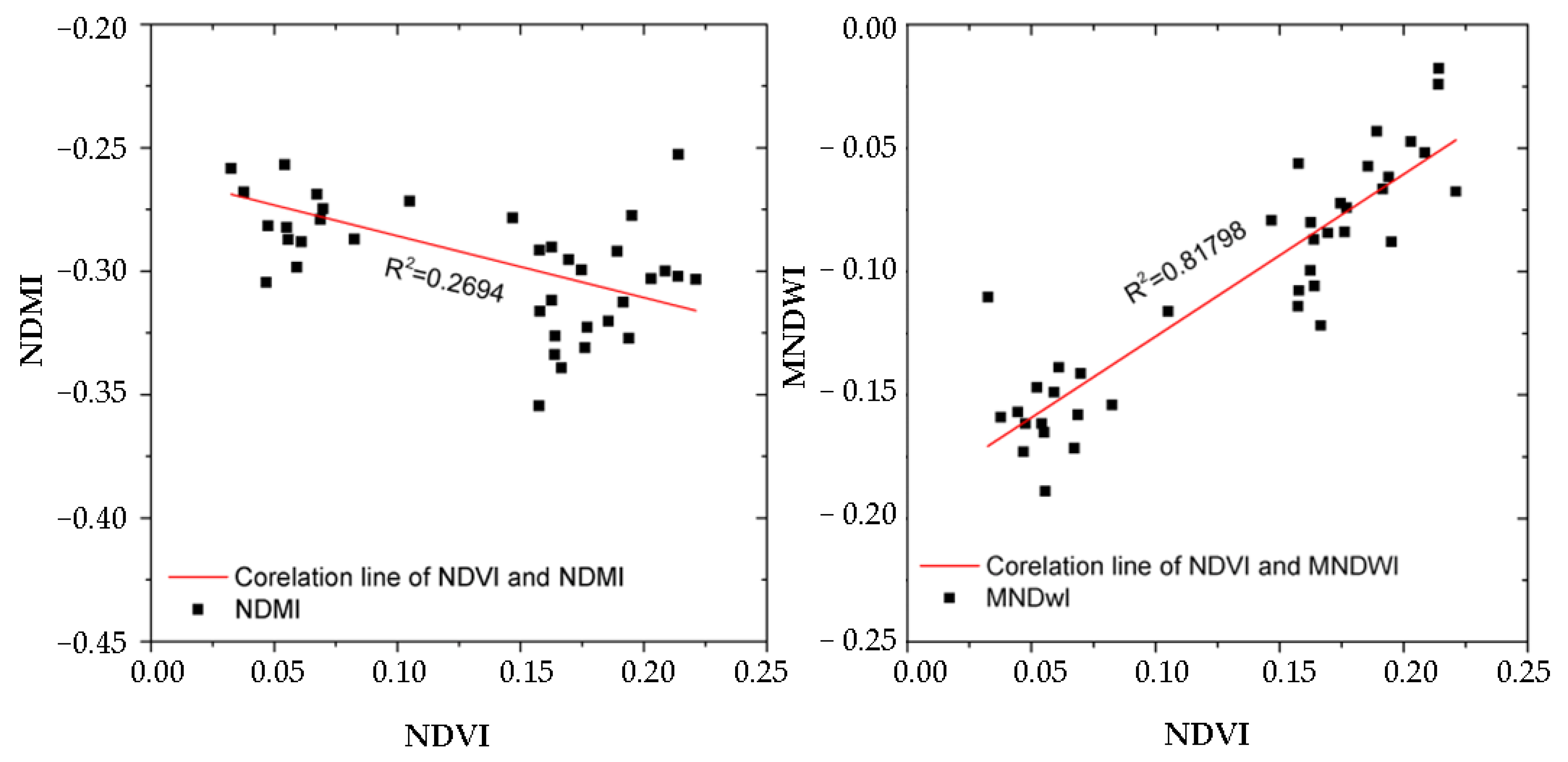
In the inundated area depicted by the rectangular area in Figure 6, Figure 7 and Figure 8, a time series of NDVI, MNDWI, and NDMI is also displayed in Figure 9 for the months of February through December of 2020. The result demonstrates that both NDVI and MNDWI values decreased just after the event over the flood affected area. However, NDMI does not follow a similar trend. In order to evaluate the relationship between the indices, we illustrated the correlation between NDVI, MNDWI, and NDMI in Figure 10. It is clear from Figure 10 that NDMI and NDVI have a weak negative correlation (R2 = 0.27). NDVI and MNDWI, on the other hand, show a high positive correlation (R2 = 0.82).
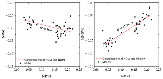
Figure 10.
Correlation graphs between NDVI and NDMI and MNDWI.
It is possible to identify the changes by using most of the stated spectral water indices due to the impact of the flood on the affected area by manipulating the color table to some extent. These results indicate that the flood-inundated areas can be detected not only by MNDWI but also by NDVI. Furthermore, the NDVI has a higher spatial resolution (10 m) compared to those of MNDWI (20 m) and NDMI (20 m) because the spatial resolution of the SWIR band is 20 m in the Sentinel-2 images. Higher spatial resolution images are expected to detect the inundation areas in more detail. For those reasons, we intend to employ the NDVI applicability in detecting flood-inundated areas in this study.
3.2. Relative Difference in NDVI (rdNDVI)
It is self-evident that the information contained in any given index varies substantially depending on the seasons and type of land cover, such as vegetation types. As a result, using a single indicator to assess complex landscapes is technically difficult because change does not always correlate to the degree of effects [56]. It is difficult to quantify changes in fractional forest, grass, or shrub cover because an NDVI drop in a low-NDVI drought-sensitive open forest area can have a greater impact than a similar percent loss in a high-NDVI dense forest [57]. Hence, rdNDVI [58] was calculated using the Equation (5),
In Equation (5), NDVIPre and NDVIPost present the greenest pixel composites in multitemporal pre- and post-event satellite imagery, respectively. Equation (2) was originally used to help not only interpret or quantify the changes in complex landscapes such as fractional forest, grass, or shrub cover, particularly with low-resolution imagery, but also help partially overcome problems that arise from NDVI’s nonlinear responsiveness or NDVI “saturation” effect [58]. When forest cover is low, a few trees added (or lost) have a higher impact on NDVI than a few trees lost in a dense forest cell. When both areas experience the same absolute change in NDVI, taking the square root of the denominator makes cells with high and low NDVI values fall more similarly. The result of Equation (5) represents a normalized percentage of NDVI gained or lost. Later, Scheip et al. [25] used the rdNDVI technique to detect surface changes, primarily vegetation area changes, as a result of fire, volcanic eruptions, and landslides. Scheip et al. [25] never discuss the feasibility of the method in detecting flood-inundated areas, particularly in non-vegetated areas, unlike the current work. This study will focus on the feasibility of the rdNDVI-based detection, delineation, and assessments of inundated areas in the non-vegetated arid region of Charikar, Afghanistan.
We prepared two temporal composites. One is a stack of all pre-event images, and the second contains all post-event images. Then, we calculated pre- and post -event NDVI for the so-called stacks. The greenest-pixel composite is a single composite or tiled image generated from all images within the user-defined pre- and post-event windows that record the pixel with the highest NDVI result as shown in Equation (1). Instead of differencing true-color composites such as red, green, and blue bands, it exploits changes in surface vegetation by developing and differencing an NDVI band from the greenest-pixel composite image. Simply, the algorithm works in a way that from all-composite images it retains only the pixels with the highest NDVI value from the entire stack. This composite indicates the peak phenological cycle of pre- and post-event conditions. The rdNDVI indicator was derived by using the peak phenological cycle calculated from the user input duration (in months) for the pre- and post-event duration.
3.3. Histogram-Based Segmentation
The thresholding-based segmentation algorithm is one of the simplest, most powerful, and most commonly used algorithms for the segmentation process. A thresholding value is applied to histograms based on segmentation. This technique is used to segment the area of interest (AOI) from images with a uniformly bright background. Based on AOI, the threshold might have a single or multiple values. The entire image is pixel-by-pixel scanned in order to designate pixels as objects or background according to gray-level value and thresholding function (T). In the current study, to discriminate between the inundated and non-inundated area pixels, we used a histogram-based thresholding technique to find a set of thresholds. The method associates each pixel of the image (f) with a binary number that depends on the intensity of the pixels and a threshold T:
The above equation simply defines the binarization method. The thresholding process produces a binary image as its output. In Equation (6), pixels with an intensity value of 1 correspond to objects (inundated area), whereas pixels with a value of 0 correspond to the background (non-inundated area). In histogram-based thresholding, it is critical to select the optimum threshold, and this process needs to be carried out in a way that produces the least amount of bias possible. The optimal value was obtained manually by iterating the value and observing the outcome. This process was repeated until we observed that, with the value that was selected, the image contained almost all of the pixels that were present in the original image. The histogram-based methods typically produce results that contain noise that needs to be removed before further analysis can be performed. In this specific research area, we use sieve analysis in ENVI 5.3 to eliminate any single separate pixel that is less than 10. It is possible to eliminate noise by using larger (11 or 12 pixel) values. However, using pixels less than 10 would diminish most of the single pixels of such size in the vicinities of the inundated area, which may underestimate the inundation area.
3.4. Accuracy Assessment Procedures Using Confusion Matrix
To validate the rdNDVI detection result, the flood inundation map was first created by using visual interpretations of pre- and post-event Sentinel-2 images, as well as governmental reports from after the flood, as shown in Figure 4. We employ a confusion matrix to evaluate the accuracy of detected inundation compared to the inundation map of the visual interpretation. Confusion matrices, also known as error matrices, are typically utilized as the quantitative method for characterizing the accuracy of image classification. These matrices contain information about actual and predicted classification. It is a table that illustrates the correspondence between the classification result and a reference image. In order to generate a confusion matrix, we require ground truth data, which consists of elements like cartographic information, images that have been manually digitized, and the outcomes of field work or surveys that have been recorded by using GPS. This data is also referred to as reference images. In this analysis, the reference image is a manually digitized version of an image that was compiled from various sources, including photographs taken after the flood, published reports, and government survey reports. It is necessary to make a comparison between the pixels that have been classified and the truth data. We have two classes of inundated and non-inundated areas that were produced by using binarization thresholding methods. As a means of performing the accuracy assessment, we made use of the outcome of the visually identified inundated reference map data. The estimated inundated pixels located within the boundary of the reference map (visually identified inundated map) is the number of correctly identified pixels. On the basis of the confusion matrix, a pixel-by-pixel analysis of the image’s accuracy was carried out. We present the accuracy of the result by considering the user’s accuracy, the producer’s accuracy, the overall accuracy, and the kappa coefficient.
3.5. Flood Susceptibility Mapping Model Based on Flow-R
Remote sensing technology is a very useful tool for detecting and monitoring land-use changes after natural disasters. However, evaluation and prediction of hazardous areas for flooding are also important issues in considering countermeasures for future events. In order to talk about how well the simulation method works for figuring out flood inundation areas for future flash floods, semi-automatic debris flood-mapping susceptibility is made by using Flow-R and free DEM from ASTER Global DEM (ASTER-GDEM) [59] with 30 m spatial resolution (see Figure 4). Flow-R is a freely available simulation software developed by [31] that has been used to simulate the flow propagation of debris flows and debris floods through a DEM. The Flow-R software is a path assessment of gravitational hazards that provides a substantial basis for a preliminary susceptibility assessment at a regional scale [31]. It has been successfully applied to different case studies in various countries with variable data quality and satisfying accuracy. We utilized the Flow-R simulation to discuss the applicability of the technique in assessing flood areas for a future event. Although in this study, Flow-R is applied to a true disaster, such a simulation technique is especially useful to identify vulnerable areas before the sources of an event are provided. The main input requires two steps to apply the technique. First, we need to provide source points by using morphological and/or user-defined criteria. Second, debris floods are being propagated from the given source points based on simple frictional laws and flow spreading algorithms. Debris floods are caused by water moving quickly through steep channels with a lot of debris in them. Their peak flow is similar to that of water floods [60].
The DEM used for the simulation of flood susceptible areas was 30 m, which is a very low resolution. However, the developer of the Flow-R [31] reported that the quality of the produced map is of major importance for the result’s accuracy. In addition, Horton et al. [31], suggest that a DEM resolution of 10 m is a good compromise between the amount of time it takes to process the data and the quality of the results. In addition, the hazard map that is generated by Flow-R is a possible future hazard map, which means that compatibility of one hundred percent is not required to be achieved. Because it only shows the areas that could potentially be hazardous. For Flow-R analysis, we follow the methods described by [31].
4. Results
We identify the flood inundation area by using the GEE in Section 4.1. The inundation map by visual interpretation is discussed in Section 4.2, and the accuracy assessment using the confusion matrix is presented in Section 4.3.
4.1. Extraction of Flood-Inundated Areas
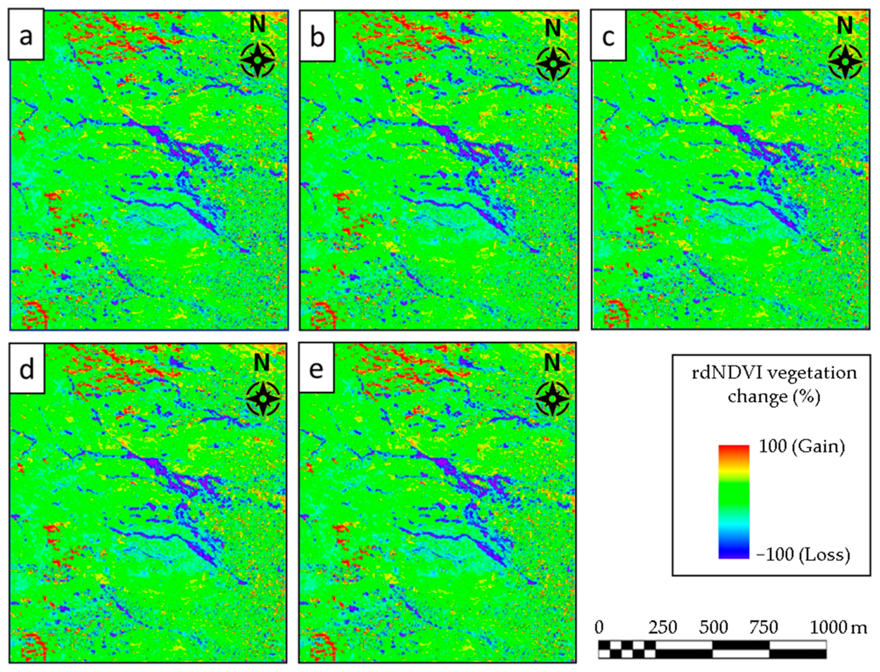
As discussed in the previous chapter, we initially chose two months for the pre-event and two months for the post-event periods. There were 14 photos available for the given time period. We took into account the total pre-event images, and we altered the number of post-event images during the study to evaluate and determine the least duration that the rdNDVI can analyze and identify the affected area. We started by analyzing all pre-event composites into a single post-event image, as shown in Figure 11a. In the subsequent stages of analysis, two post-event images are taken, and in the final iteration, we compare all pre-event images to all post-event data in the study area, as shown in Figure 11a–e.
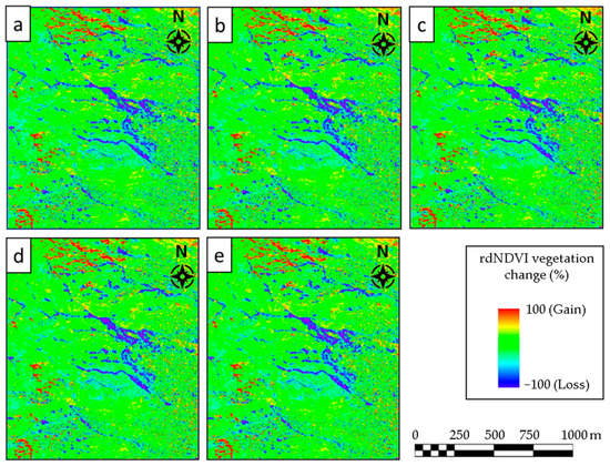
Figure 11.
The figure depicts the result of the rdNDVI map for five scenarios. Pre-and post-event images were acquired between 5 June 2020 and 31 October 2020. Figures (a) through (e) show the rdNDVI results for all available pre- and post-event images used in this study. (a) presents the result of rdNDVI, which was generated with only one post-image acquired on 13 September 2020. (b–e) represent the results obtained from two, three, four, and five post-event images, respectively.
Figure 11 presents the rdNDVIs’ inundation map where the blue color illustrates the decrease of NDVI as a result of the flood event. The colors other than blue show no change (green) and vegetation gain (red). From Figure 11, it can be clearly seen that by considering only one post-event image, we obtained a clear inundation map. By increasing the number of the post-event images, we noticed slight changes in the result of the inundation map. The changes were so small that they were barely noticeable without a close-up of the image. Therefore, we can conclude that by using only one post-event image, we can detect the flooded area by using the rdNDVI algorithm. For further analysis, we use the image presented in Figure 11a.
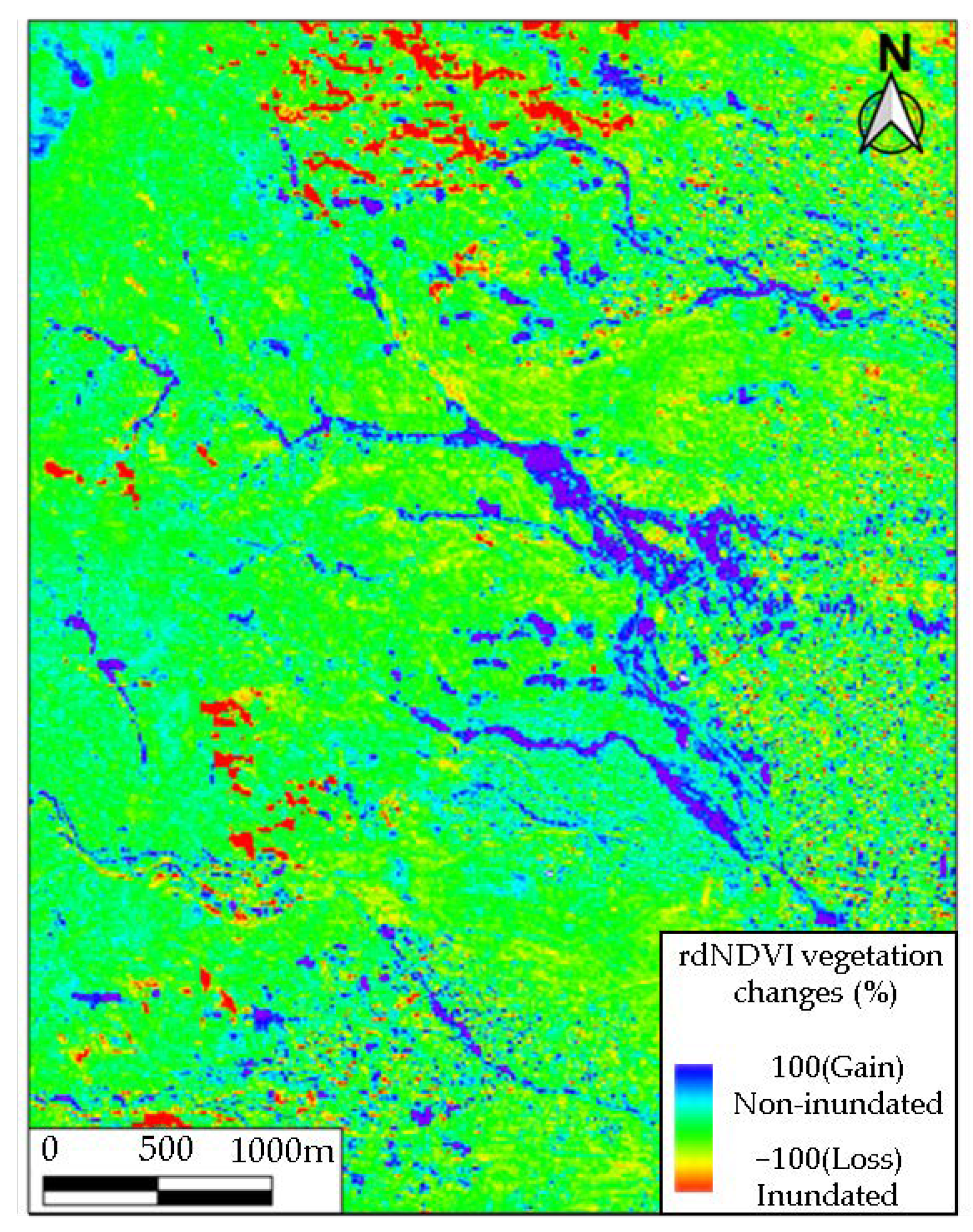
Figure 12 presents the larger map of the rdNDVI vegetation change in percentage. The blue color represents the loss of vegetation, which here means inundated areas, whereas red colors indicate vegetation gain or non-flooded areas’ detection. As can be seen, the current technique rapidly detects the inundated area by using the explained methodology. However, there were falsely detected areas due to the existence of a sharp slope that reflected as a shadow. Hence, we canceled out those undesired noises by using sieve analysis. We also masked out falsely detected areas resulting from sharp slopes (greater than 30 degrees).
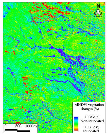
Figure 12.
rdNDVI-based change detection image and greenest pixel composites (pre-event time: 2-months; post-event time: 16 days).
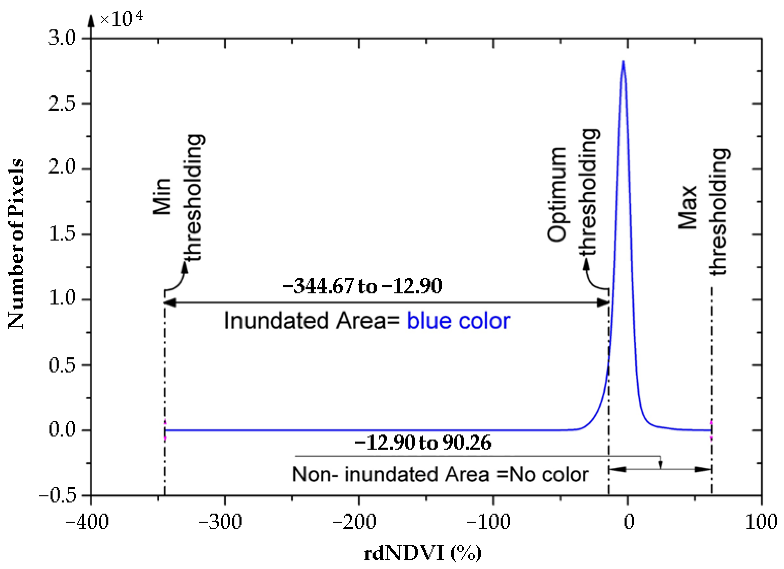
To conduct an error assessment, we first simplified the representation of the inundated image into an easily distinguishable map. We used a histogram-based thresholding technique, as explained in the methodology, to find a set of thresholds that can discriminate between the inundated and background pixels, as presented in Figure 13.

Figure 13.
Histogram of the rdNDVI image with the chosen thresholds.
Figure 13 presents the histogram of the rdNDVI image with the minimum, optimum, and maximum thresholding. We segmented the image based on the optimum thresholding of −12.90 into two different colors. The optimum value was obtained manually by iterating the value and observing the result. This process was repeated until we noticed that, with the selected value, the image contained nearly all of the pixels from the original image. For values smaller than the optimum value, we chose the color to be blue, which represents the inundated area. Values larger than optimum thresholding were segmented into a non-inundated area which is presented in white or non-color. The result of binarization is illustrated in Figure 14a, which only consists of two classes of inundated and non-inundated zones. However, the result of threshold binarization contains unwanted salt-and-pepper noise. We mask out the so-called unwanted noises with a 10-pixel size (Figure 14b). All noises with small areas were canceled out by using the sieve analysis in ENVI 5.3 software, as shown in Figure 14b. Figure 14b shows the final inundation map of Charikar, which occurred on 26 August 2020. A total of 300 hectares of built-up area were extracted as inundations.
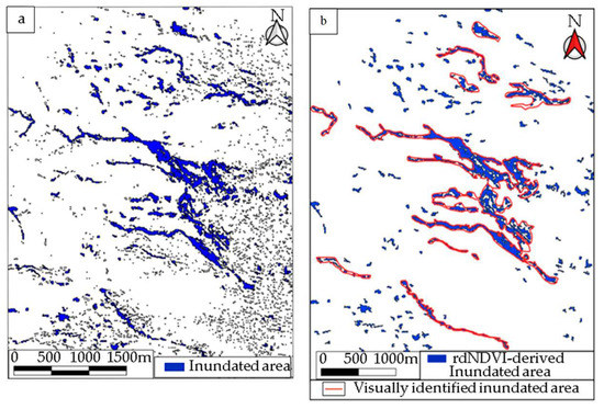
Figure 14.
The extraction of inundated and non-inundated areas from the rdNDVI result based on binarization for two thresholds. (a) The left image presents the result of threshold binarization with unwanted salt-and-pepper noise. (b) In the left image, the inundated area (shown by the red lines) is superimposed on the extracted image of the threshold-binarization after removing salt-and-pepper noise.
4.2. Inundation Map by Visual Interpretation
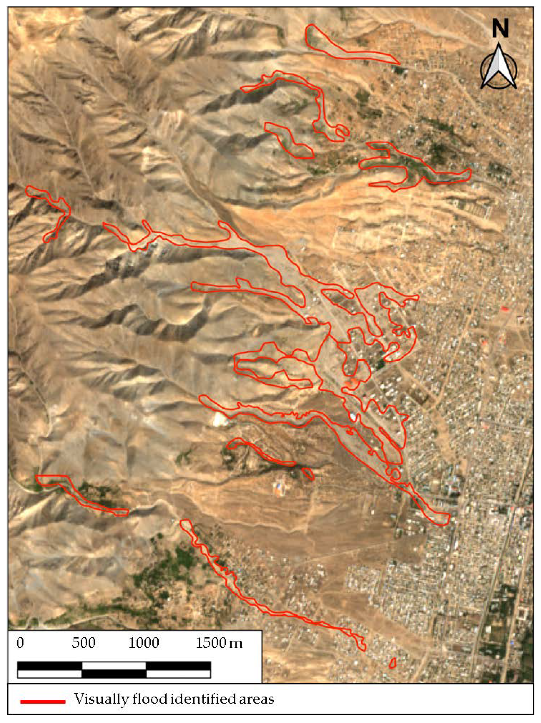
To draw the true inundation of Charikar, we collected the reports published mainly in the local language by the Disaster Management Authority, the National Statistic and Information Authority (NSIA) [61], and the National Water Affairs Regulation Authority. Moreover, we visually compared the pre- and post-event satellite images side by side to identify changes between the flood events. We used the Sentinel-2 satellite images acquired before the event (24 August 2020) and after the event (13 September 2020) as reference data. We overlaid the true Charikar inundated vector data, which is similar to the true impacted site. Because of the resolution of the satellite images, only significant changes were considered. Therefore, minor damage may not be visible, and it was neglected in this study. Although the inundation area by the Charikar flood was also estimated by visual interpretation in a previous study [62], the interpreted area was limited. We estimated the inundation map for a wider area. In the visual interpretation process, we considered the previous inundated map in [62] and the reports by the government authorities. The official reports by the government were reflected in the inundation map. For example, when building damage was reported in some towns in the official documents, inundation areas were identified in the town by the visual interpretations. Figure 15 presents the result of our visual interpretation.

Figure 15.
Visual interpretation of the flood-inundated area. Image drawn from our visual interpretation with government reports.
4.3. Accuracy Assessment
The accuracy assessment of the results obtained in this study was made through a confusion matrix explained in the methodology. We overlaid the result of the rdNDVI-based change detection shown in Figure 14b on the visually identified inundation map shown in Figure 15. The error assessment was conducted pixel-by-pixel based on the confusion matrix. The result of the confusion matrix is presented in Table 2. It presents the user’s accuracy, the producer’s accuracy, the overall accuracy, and the kappa coefficient. The accuracy assessment obtained from the analysis of this study shows an overall accuracy of 88.44% with a kappa coefficient of 0.75, which indicates a good agreement between thematic maps generated from images and the reference data.
Table 2.
Accuracy assessment result using the confusion matrix.
Based on the inundated map obtained in this study, most of the affected houses were in built-up areas, and it was also confirmed by government reports. Another significant point of this method is the ability to detect changes with a single post image. Increasing the number of post-event images does not increase the quality of the detected image. Therefore, the rdNDVI algorithm has the potential to quickly identify the flood-affected area immediately after an event on a routine basis, typically with comparable accuracy to on-site reports, to help decision makers find a quick way to contribute significantly to the post-disaster activities.
5. Discussion
This section discusses the monitoring of the changes in the affected area after two years in Section 5.1, flow propagation analysis by Flow-R in Section 5.2, and the practical use of the method and future aspects in Section 5.3.
5.1. Monitoring the Changes in the Affected Area in Two Years
We have noticed a significant improvement in the spatial resolution of the remote sensing data which is available to governments in the state or local and regional governments. It is very helpful for the public sector and local governments to consider the use of new remote sensing technologies to monitor and efficiently act based on needs. The use of satellite data and remote sensing applications already brings significant efficiency to the decision-makers and policymakers of developed countries. However, developing countries such as Afghanistan do not have the technical capacity to use remote sensing data and applications for post-disaster activities. In most cases, even having information about the affected area, the government does not reach out to the people to help them in the recovery process.
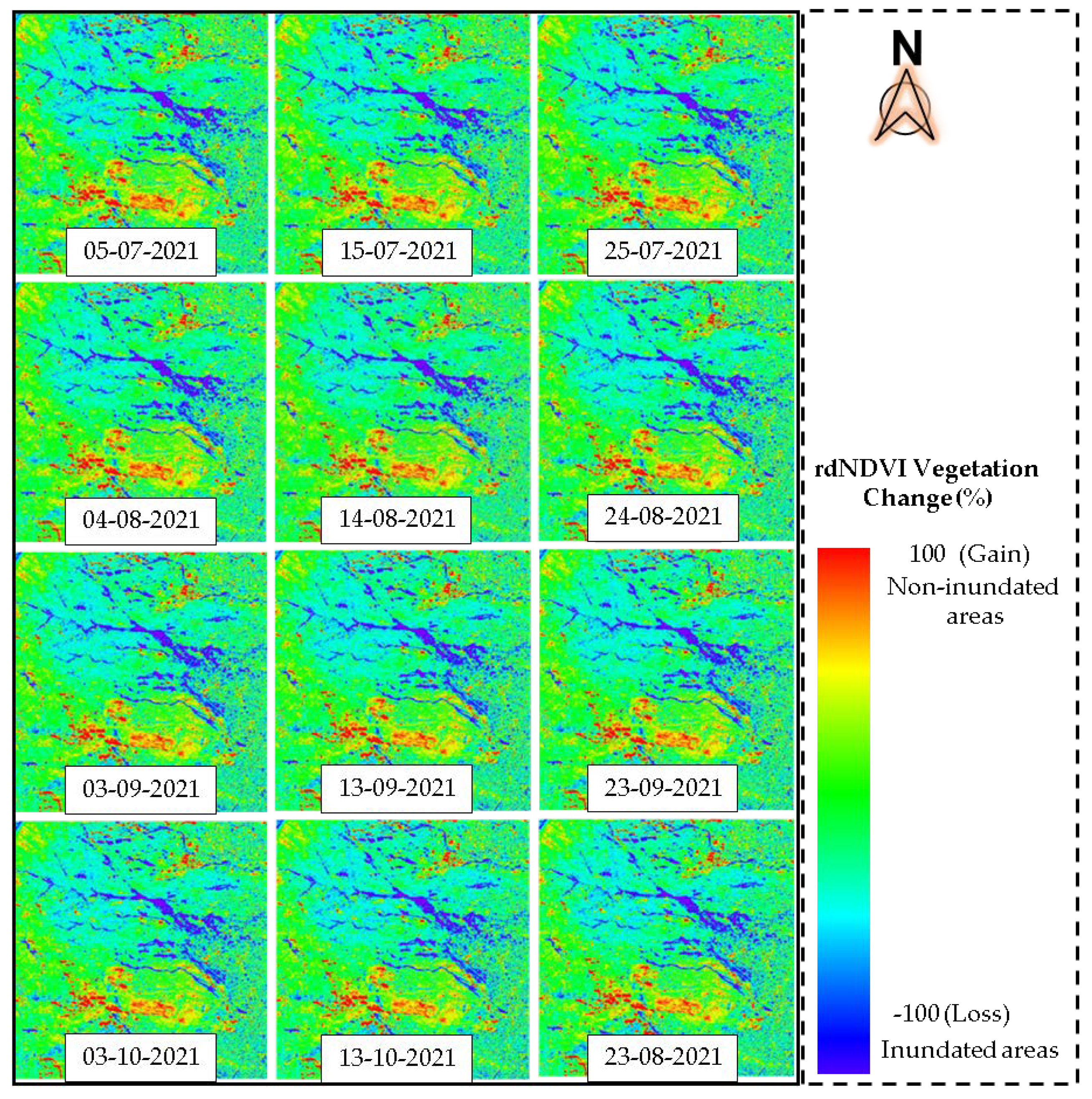
Figure 16 and Figure 17 are presented to show the changes in the study area after the event over a long period of time. From the NDVI time series (Figure 16) in the typically affected area shown by the rectangular area in Figure 5, Figure 6, Figure 7 and Figure 8, we noticed that the NDVI decreased after the event in Charikar. As can be seen, even after one year, the NDVI values did not recover. We illustrate the rdNDVI changes one year after the event in Figure 17. We observed very small and negligible changes in the rdNDVI image time series, indicating that the affected area has not yet been significantly recovered. Probably one factor behind the lack of changes in the NDVIs is the limitation of economic and human resources in the Afghanistan government, which they failed to utilize to revitalize and rebuild the affected areas. People also could not rebuild their houses, probably due to their poverty. This result shows that the NDVI and rdNDVI techniques are very useful for monitoring the event, and it will be particularly useful to observe how long it will take for the recovery of the affected area.
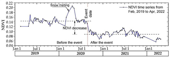
Figure 16.
NDVI time series over the study area; the blue line indicates the raw NDVI from February 2019 to April 2022.
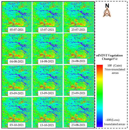
Figure 17.
rdNDVI changes in Charikar after a one-year period.
5.2. Flow Propagation Analysis by Flow-R
The freely available ASTER-GDTM with 30 m spatial resolution was used in the simulation of the Charikar flood event. The initial pixels of the detected inundated areas in the mountains were selected as the predefined source points. The parameters for flow spreading in Flow-R were provided as shown in Table 3.
Table 3.
Debris-flood parameters used in Flow-R.
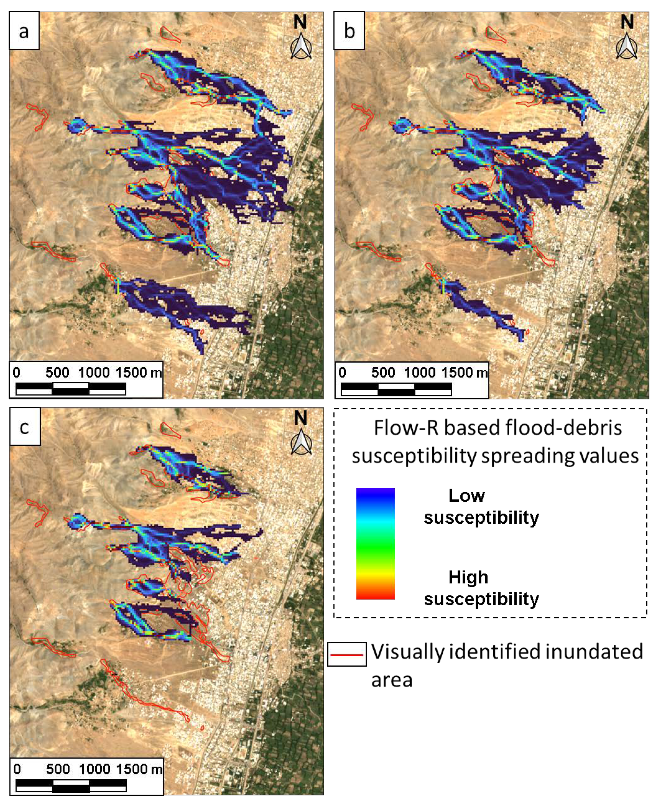
These parameters were also used in the evaluation of the debris-flow events in Hiroshima prefecture, Japan in July 2018 [63]. We considered three different travel angle iterations for the analysis, as illustrated in Table 3, because the threshold of the travel angle largely controls the propagation areas. The result of each iteration is shown in Figure 18. The overlaid red lines are the visually identified inundation maps. The findings demonstrate that the estimated regions of spreading successfully reproduced the inundated areas caused by the flood. We noticed that smaller travel angles such as four degrees overestimated the inundation areas, as shown in Figure 18a, and larger travel angles, such as six degrees, underestimated the flood inundation areas (Figure 18c). The result with a travel angle of five degrees, shown in Figure 18b, gave moderate spreading areas. Figure 18b depicts a spread region that is slightly bigger than the inundation areas that were determined, but the simulation that used a travel angle of five degrees was able to better reproduce these inundation areas. These results indicate that hazardous areas for future flood events can be evaluated if appropriate source points are provided in the simulation. Such simulations would be useful not only for government officials but also for residents living in natural hazard-susceptible areas, particularly flood- and debris-flow-prone areas, to increase their awareness of mitigating future disasters.

Figure 18.
Flow-R generated flood-debris susceptibility map using a four-degree travel angle illustrated in (a), five-degree travel angle in (b), and six-degree travel angle in (c).
5.3. Practical Use of the Method and Future Aspects
As discussed in this study, we found a strong similarity between NDVIs and MNDWIs in the flood inundation areas. Because the spatial resolution of NDVI is higher than MNDWI in most optical satellite images, including the Sentinel-2, NDVI would be a powerful index in precisely detecting inundation areas for a semi-arid region such as Afghanistan even if water bodies derived from floods do not exist in the affected area. Because most optical satellite sensors, including high-resolution satellites, obtain near-infrared band, and only specific satellites, such as Landsat and Sentinel-2, have short-wavelength infrared band limits, NDVI is a more common and practical index, indicating that an NDVI-based approach can be applied to various optical images. The GEE also allows us to automatically assess the land cover change based on rdNDVI with minimum effort in preprocessing of the satellite images. It means that inundation areas would be quickly estimated immediately after a disaster if a cloud-free optical image is obtained immediately following the event. In order to further assess structural damage such as buildings and infrastructures such as roads and bridges in natural disasters, spatial databases in geographic information systems (GIS) would be useful not only at local and regional levels but also at global level [64,65,66,67,68,69]. By superimposing the building and infrastructure inventory data in the GIS database on the inundation map developed by the proposed method, the amount and extent of the structural damage can be easily evaluated. Although up-to-date GIS databases have not fully developed, especially in developing countries, mainly due to financial problems, the recent development of open geographical databases such as OpenStreetMap (OSM) [70] and satellite image-derived topographical data [59] would allow us to freely use the spatial datasets and to develop damage maps in natural disasters.
The identification of flood inundation areas, and the distribution of the affected areas including building and infrastructure damage maps are an essential part of post-disaster activities such as rescuing impacted individuals, providing more vital relief, and helping communities in the reconstruction of affected areas. Furthermore, the identification of flood-prone areas for future events by simulation techniques such as Flow-R would be beneficial in considering risk reduction measures not only for urban planners and policymakers but also for residents living in the dangerous areas. The results of the remote sensing-based assessments and the prediction of high-risk areas would enhance government and official awareness of future natural disasters.
6. Conclusions
This study examined the applicability of the rdNDVI technique in Sentinel-2 images to estimate the flood inundation areas in a semi-arid region by using the GEE. The methodology of this study was applied to the flash flood event in Charikar, Afghanistan on 26 August 2020. We examined several spectral indices such as NDVI, MNDWI, and NDMI in detecting the inundation areas. We found a strong correlation between NDVI and MNDWI, and both indices decreased significantly in the impacted regions immediately after the incident. On the contrary, NDMI did not show any remarkable change before and after the event. From the viewpoint of the spatial resolution, we determined to use NDVI in detecting the inundation areas. One of the important conclusions of this work is that NDVI worked effectively in delineating flood inundation areas in a semi-arid region.
The analysis of the rdNDVIs between the pre- and post-event images showed that the inundation areas were adequately extracted by using a single post-event image. The binarization based on the histogram of the rdNDVIs and the removal of isolated noise were applied to develop the inundation map. The total flood-affected area estimated by the current method was approximately 300 ha. From the comparison with the visually interpreted inundation areas, we found that the inundation areas were successfully detected with an overall accuracy of 88% and a kappa coefficient of 0.75. The results show that the inundation areas were accurately detected by the rdNDVI technique even in semi-arid places like Charikar, where there isn’t much vegetation.
The time-series analysis of the NDVIs two years after the flash flood event revealed that there was no significant change in the NDVIs in the affected areas, most likely due to a lack of financial and human resources in the government and the poverty of the affected residents. In addition, we discussed the potential of the flow propagation prediction technique in Flow-R for identifying flood prone areas by using the ASTER GDEM with a spatial resolution of 30 m. We revealed that the inundation areas of the Charikar event were successfully reproduced by the Flow-R-based simulation by providing starting points in the actual event.
Satellite image- and/or DEM-based approaches would be beneficial in performing pre-and post-disaster activities, especially for countries with fewer financial and human resources such as Afghanistan. Implementations of remote sensing technologies including the proposed method in this study to the government and official agencies would be a key for more rapid and adequate disaster responses and effective countermeasures against future natural disasters.
Author Contributions
M.R.A. and H.M. conceived, designed, performed the experiments, and wrote the manuscript. All authors have read and agreed to the published version of the manuscript.
Funding
This research was funded by the Japan Society for the Promotion of Science (KAKENHI grant numbers 19H02408 and 22H01741).
Data Availability Statement
The data that support the findings of this study are available from the authors, upon reasonable request.
Acknowledgments
The author would like to take this chance to thank the MEXT (Ministry of Education, Culture, Sports, Science, and Technology) Scholarship of Japan, which gave him a full scholarship to study for his doctorate at Hiroshima University.
Conflicts of Interest
The authors declare no conflict of interest.
References
- United Nations International Strategy for Disaster Reduction (UNISDR). The Human Cost of Weather-Related Disaster 1995–2015. Available online: https://www.preventionweb.net/publication/human-cost-weather-related-disasters-1995-2015 (accessed on 12 March 2022).
- Freebairn, A.; Turmine, V.; Singh, R. Climate as a risk multiplier-trends in vulnerability and exposure. In World Disasters Report 2020 Come Heat or High Water; Hagon, K., Ed.; IFRC: Geneva, Switzerland, 2020; pp. 119–126. [Google Scholar]
- Embabi, N.S. The Geomorphology of Egypt: Landforms and Evolution: The Nile Valley and the Western Desert; Egyptian Geographical Society: Cairo, Egypt, 2004; Volume 1. [Google Scholar]
- Chin, A.; Gregory, K.J. Urbanization and adjustment of ephemeral stream channels. Ann. Assoc. Am. Geogr. 2001, 91, 595–608. [Google Scholar] [CrossRef]
- Khosravi, K.; Shahabi, H.; Pham, B.T.; Adamowski, J.; Shirzadi, A.; Pradhan, B.; Dou, J.; Ly, H.-B.; Gróf, G.; Ho, H.L.; et al. A comparative assessment of flood susceptibility modeling using Multi-Criteria Decision-Making Analysis and Machine Learning Methods. J. Hydrol. 2019, 573, 311–323. [Google Scholar] [CrossRef]
- Muis, S.; Güneralp, B.; Jongman, B.; Aerts, J.C.J.H.; Ward, P.J. Flood risk and adaptation strategies under climate change and urban expansion: A probabilistic analysis using global data. Sci. Total Environ. 2015, 538, 445–457. [Google Scholar] [CrossRef] [PubMed]
- Wu, W.; Westra, S.; Leonard, M. A basis function approach for exploring the seasonal and spatial features of storm surge events. Geophys. Res. Lett. 2017, 44, 7356–7365. [Google Scholar] [CrossRef]
- Zaji, A.H.; Bonakdari, H.; Gharabaghi, B. Remote sensing satellite data preparation for simulating and forecasting river discharge. IEEE Trans. Geosci. Remote Sens. 2018, 56, 3432–3441. [Google Scholar] [CrossRef]
- El Hames, A.; Richards, K.S. An integrated physically based model for arid region flash flood prediction capable of simulating dynamic transmission loss. J. Hydrol. Process. 1998, 12, 1219–1232. [Google Scholar] [CrossRef]
- Walling, D.E.; Gregory, K.J. The measurement of the effects of building construction on drainage basin dynamics. J. Hydrol. 1970, 11, 129–144. [Google Scholar] [CrossRef]
- McFeeters, S.K. The use of the Normalized Difference Water Index (NDWI) in the delineation of open water features. Int. J. Remote Sens. 1996, 17, 1425–1432. [Google Scholar] [CrossRef]
- Rogers, A.S.; Kearney, M.S. Reducing signature variability in unmixing coastal marsh Thematic Mapper scenes using spectral indices. Int. J. Remote Sens. 2004, 25, 2317–2335. [Google Scholar] [CrossRef]
- Xu, H. Modification of normalized difference water index (NDWI) to enhance open water features in remotely sensed imagery. Int. J. Remote Sens. 2006, 27, 3025–3033. [Google Scholar] [CrossRef]
- Feyisa, G.L.; Meilby, H.; Fensholt, R.; Proud, S.R. Automated water extraction index: A new technique for surface water mapping using Landsat imagery. Remote Sens. Environ. 2014, 140, 23–35. [Google Scholar] [CrossRef]
- Wang, S.; Baig, M.H.A.; Zhang, L.; Jiang, H.; Ji, Y.; Zhao, H.; Tian, J. A simple enhanced water index (EWI) for percent surface water estimation using Landsat data. IEEE J. Sel. Top. Appl. Earth Obs. Remote Sens. 2014, 8, 90–97. [Google Scholar] [CrossRef]
- Rokni, K.; Ahmad, A.; Selamat, A.; Hazini, S. Water feature extraction and change detection using multitemporal Landsat imagery. Remote Sens. 2014, 6, 4173–4189. [Google Scholar] [CrossRef] [Green Version]
- Duan, Z.; Bastiaanssen, W.G.M. Estimating water volume variations in lakes and reservoirs from four operational satellite altimetry databases and satellite imagery data. Remote Sens. Environ. 2013, 134, 403–416. [Google Scholar] [CrossRef]
- Davranche, A.; Lefebvre, G.; Poulin, B. Wetland monitoring using classification trees and SPOT-5 seasonal time series. Remote Sens. Environ. 2010, 114, 552–562. [Google Scholar] [CrossRef] [Green Version]
- Poulin, B.; Davranche, A.; Lefebvre, G. Ecological assessment of Phragmites australis wetlands using multi-season SPOT-5 scenes. Remote Sens. Environ. 2010, 114, 1602–1609. [Google Scholar] [CrossRef] [Green Version]
- Huete, A.R.; Liu, H.Q.; Batchily, K.; van Leeuwen, W. A comparison of vegetation indices over a global set of TM images for EOS-MODIS. Remote Sens. Environ. 1997, 59, 440–451. [Google Scholar] [CrossRef]
- Escuin, S.; Navarro, R.; Fernández, P. Fire severity assessment by using NBR (normalized burn ratio) and NDVI (normalized difference vegetation index) derived from LANDSAT TM/ETM images. Int. J. Remote Sens. 2008, 29, 1053–1073. [Google Scholar] [CrossRef]
- Sidi Almouctar, M.A.; Wu, Y.; Kumar, A.; Zhao, F.; Mambu, K.J.; Sadek, M. Spatiotemporal analysis of vegetation cover changes around surface water based on NDVI: A case study in Korama basin, Southern Zinder, Niger. Appl. Water Sci. 2021, 11, 4. [Google Scholar] [CrossRef]
- Huang, C.; Chen, Y.; Zhang, S.; Wu, J. Detecting, extracting, and monitoring surface water from space using optical sensors: A review. Rev. Geophys. 2018, 56, 333–360. [Google Scholar] [CrossRef]
- DeVries, B.; Huang, C.; Armston, J.; Huang, W.; Jones, J.W.; Lang, M.W. Rapid and robust monitoring of flood events using Sentinel-1 and Landsat data on the Google Earth Engine. Remote Sens. Environ. 2020, 240, 111664. [Google Scholar] [CrossRef]
- Scheip, C.M.; Wegmann, K.W. HazMapper: A global open-source natural hazard mapping application in Google Earth Engine. Nat. Hazards Earth Syst. Sci. 2021, 21, 1495–1511. [Google Scholar] [CrossRef]
- Saah, D.; Tenneson, K.; Matin, M.; Uddin, K.; Cutter, P.; Poortinga, A.; Nguyen, Q.H.; Patterson, M.; Johnson, G.; Markert, K.; et al. Land cover mapping in data scarce environments: Challenges and opportunities. Front. Environ. Sci. 2019, 7, 150. [Google Scholar] [CrossRef] [Green Version]
- Phongsapan, K.; Chishtie, F.; Poortinga, A.; Bhandari, B.; Meechaiya, C.; Kunlamai, T.; Aung, K.S.; Saah, D.; Anderson, E.; Markert, K.; et al. Operational flood risk index mapping for disaster risk reduction using earth observations and cloud computing technologies: A case study on Myanmar. Front. Environ. Sci. 2019, 7, 191. [Google Scholar] [CrossRef] [Green Version]
- Poortinga, A.; Nguyen, Q.; Tenneson, K.; Troy, A.; Saah, D.; Bhandari, B.; Ellenburg, W.L.; Aekakkararungroj, A.; Ha, L.; Pham, H.; et al. Linking earth observations for assessing the food security situation in Vietnam: A landscape approach. Front. Environ. Sci. 2019, 7, 186. [Google Scholar] [CrossRef] [Green Version]
- Patel, N.N.; Angiuli, E.; Gamba, P.; Gaughan, A.; Lisini, G.; Stevens, F.R.; Tatem, A.J.; Trianni, G. Multitemporal settlement and population mapping from Landsat using Google Earth Engine. Int. J. Appl. Earth Obs. Geoinf. 2015, 35, 199–208. [Google Scholar] [CrossRef] [Green Version]
- Mutanga, O.; Kumar, L. Google Earth Engine applications. Remote Sens. 2019, 11, 591. [Google Scholar] [CrossRef] [Green Version]
- Horton, P.; Jaboyedoff, M.; Rudaz, B.; Zimmermann, M. Flow-R, a model for susceptibility mapping of debris flows and other gravitational hazards at a regional scale. Nat. Hazards Earth Syst. Sci. 2013, 13, 869–885. [Google Scholar] [CrossRef] [Green Version]
- Atefi, M.R.; Miura, H. Detection and Volume Estimation of Large-Scale Landslide in Abe Barek, Afghanistan Using Nonlinear Mapping of DEMs. In Proceedings of the 2021 IEEE International Geoscience and Remote Sensing Symposium IGARSS, Brussels, Belgium, 11–16 July 2021; pp. 3757–3760. [Google Scholar] [CrossRef]
- Atefi, M.R.; Miura, H. Volumetric analysis of the landslide in Abe Barek, Afghanistan based on nonlinear mapping of stereo satellite imagery-derived DEMs. Remote Sens. 2021, 13, 446. [Google Scholar] [CrossRef]
- Tolo News Reporters’ Team. Over 110 killed in flash floods in Afghanistan. Tolo News. 27 August 2020. Available online: https://tolonews.com/afghanistan/over-110%C2%A0killed-flash-floods-afghanistan (accessed on 2 March 2022).
- Gibbons, T.; Fahim Abed, N. Nearly 80 killed as flash floods ravage city in Afghanistan. The New York Times. 26 August 2020. Available online: https://www.nytimes.com/2020/08/26/world/asia/afghanistan-floods-charikar.html (accessed on 2 March 2022).
- Glinski, S. Many people are still missing’: Afghanistan families devastated by flash floods. The Guardian. September 2020. Available online: https://www.theguardian.com/world/2020/sep/01/many-people-are-still-missing-afghanistan-flash-floods (accessed on 10 March 2022).
- Paikan, W. Flood in Afghanistan killed hundreds in Parwan Province. Independent Farsi. 26 August 2020. Available online: https://tinyurl.com/independentpersian (accessed on 3 March 2022).
- Gul, R. People walk near damaged houses after the 2020 heavy flooding in the Charikar, Parwan province. Fox News. 26 August 2020. Available online: https://www.foxnews.com/world/floods-in-north-east-afghanistan-leave-at-least-100-dead (accessed on 10 March 2022).
- Kohsar, W. Scores Killed, Many Still Missing after Flash Floods Ravage Afghanistan, Crumbling Homes. Cbsnews. 26 August 2020. Available online: https://www.cbsnews.com/news/flood-in-afghanistan-flash-flooding-over-100-deaths-many-missing-charikar-parwan-today-2020-08-27/ (accessed on 10 March 2022).
- Gul, R. Dozens Killed, Homes Swept Away, By Flash Floods in Afghanistan. RFE/RL Radio Azadi AP. 26 August 2020. Available online: https://www.rferl.org/a/afghanistan-weather-floods/30803355.html (accessed on 10 March 2022).
- Azadmansh, O. A general view of a building in Charikar covered with flooded debris of flooding in Parwan. Reuters. 26 August 2020. Available online: https://www.thestar.com.my/news/world/2020/08/26/flash-floods-kill-more-than-70-in-afghanistan (accessed on 10 March 2022).
- ESA Standard Document; Sentinel-2 User Handbook. European Space Agency (ESA): Paris, France, 24 July 2015. Issue 1, Revision 1. Available online: https://sentinel.esa.int/documents/247904/685211/sentinel-2_user_handbook (accessed on 10 March 2022).
- Szostak, M.; Hawryło, P.; Piela, D. Using of Sentinel-2 images for automation of the forest succession detection. Eur. J. Remote Sens. 2018, 51, 142–149. [Google Scholar] [CrossRef]
- Miranda, E.; Mutiara, A.B.; Wibowo, W.C. Classification of land cover from Sentinel-2 imagery using supervised classification technique (preliminary study). In Proceedings of the 2018 International Conference, Information Management and Technology (ICIMTech), Jakarta, Indonesia, 3–5 September 2018; pp. 69–74. [Google Scholar]
- Wang, D.; Wan, B.; Qiu, P.; Su, Y.; Guo, Q.; Wang, R.; Sun, F.; Wu, X. Evaluating the performance of Sentinel-2, Landsat-8 and Pléiades-1 in mapping mangrove extent and species. Remote Sens. 2018, 10, 1468. [Google Scholar] [CrossRef] [Green Version]
- Campos-Taberner, M.; García-Haro, F.J.; Martínez, B.; Izquierdo-Verdiguier, E.; Atzberger, C.; Camps-Valls, G.; Gilabert, M.A. Understanding deep learning in land use classification based on Sentinel-2 time series. Sci. Rep. 2020, 10, 17188. [Google Scholar] [CrossRef] [PubMed]
- Caballero, I.; Ruiz, J.; Navarro, G. Sentinel-2 satellites provide near-real time evaluation of catastrophic floods in the west Mediterranean. Water 2019, 11, 2499. [Google Scholar] [CrossRef] [Green Version]
- Dinh, D.A.; Elmahrad, B.; Leinenkugel, P.; Newton, A. Time series of flood mapping in the Mekong delta using high resolution satellite images. IOP Conf. Ser. Earth Environ. Sci. 2019, 266, 12011. [Google Scholar] [CrossRef]
- Rättich, M.; Martinis, S.; Wieland, M. Automatic flood duration estimation based on multi-sensor satellite data. Remote Sens. 2020, 12, 643. [Google Scholar] [CrossRef] [Green Version]
- Solovey, T. Flooded wetlands mapping from Sentinel-2 imagery with spectral water index: A case study of Kampinos national park in central Poland. Geol. Q. 2020, 64, 492–505. [Google Scholar] [CrossRef] [Green Version]
- Zhang, T.; Su, J.; Liu, C.; Chen, W. Potential bands of Sentinel-2A satellite for classification problems in precision agriculture. Int. J. Autom. Comput. 2019, 16, 16–26. [Google Scholar] [CrossRef] [Green Version]
- Kobayashi, N.; Tani, H.; Wang, X.; Sonobe, R. Crop classification using spectral indices derived from Sentinel-2A imagery. J. Inf. Syst. Telecommun. 2020, 4, 67–90. [Google Scholar] [CrossRef]
- Rouse, J.W.; Haas, R.H.; Schell, J.A.; Deering, D.W. Monitoring Vegetation Systems in the Great Plains with ERTS (Earth Resources Technology Satellite). In Proceedings of the 3rd Earth Resources Technology Satellite Symposium, Greenbelt, MD, USA, 10–14 December 1973; pp. 309–317. [Google Scholar]
- Hardisky, M.A.; Dauber, F.C.; Roman, C.T.; Klemas, V. Remote sensing of biomass and annual net aerial primary productivity of a salt marsh. Remote Sens. Environ. 1984, 16, 91–106. [Google Scholar] [CrossRef]
- Gao, B.C. Ndwi-a normalized difference water index for remote sensing of vegetation liquid water from space. Remote Sens. Environ. 1996, 58, 257–266. [Google Scholar] [CrossRef]
- Miller, J.D.; Thode, A.E. Quantifying burn severity in a heterogeneous landscape with a relative version of the delta Normalized Burn Ratio (dNBR). Remote Sens. Environ. 2007, 109, 66–80. [Google Scholar] [CrossRef]
- Norman, S.P.; Koch, F.; Hargrove, W.W. Review of broad-scale drought monitoring of forests: Toward an integrated data mining approach. For. Ecol. Manag. 2016, 380, 346–358. [Google Scholar] [CrossRef] [Green Version]
- Norman, S.P.; Christie, W.M. Satellite-Based Evidence of Forest Stress and Decline across the Conterminous United States for 2016, 2017, and 2018; Gen. Tech. Rep. SRS-250; US Department of Agriculture, Forest Service, Southern Research Station: Asheville, NC, USA, 2020; Volume 2020, pp. 151–166.
- NASA/METI/AIST/Japan Space systems; U.S./Japan ASTER Science Team. ASTER Global Digital Elevation Model V003; NASA EOSDIS Land Processes DAAC: Pasadena, CA, USA, 2018. [Google Scholar] [CrossRef]
- Hungr, O.; Leroueil, S.; Picarelli, L. The Varnes classification of landslide types, an update. Landslides 2014, 11, 167–194. [Google Scholar] [CrossRef]
- Reports of flood from National Statistics and Information Authority. HashtiSubh. 31 August 2020. Available online: https://8am.af/satellite-images-of-the-parwan-flood-nearly-one-thousand-houses-have-been-damaged/ (accessed on 9 March 2022).
- International Water Management Institute (IWMI). Flash Flood Hit Charikar, Parwan Province in Afghanistan, FL-2020-0006-AF version 1; International Water Management Institute (IWMI): Colombo, Sri Lanka, 26 August 2020. [Google Scholar]
- Miura, H. Fusion analysis of optical satellite images and digital elevation model for quantifying volume in debris flow disaster. Remote Sens. 2019, 11, 1096. [Google Scholar] [CrossRef] [Green Version]
- Green, D.R.; King, S.D. Applying the geospatial technologies to estuary environments. In GIS for Coastal Zone Management; Bartlett, D., Smith, J., Eds.; CRS Press: New York, NY, USA, 2005; pp. 239–255. [Google Scholar]
- Buchori, I.; Sugiri, A.; Mussadun, M.; Wadley, D.; Liu, Y.; Pramitasari, A.; Pamungkas, I.T. A Predictive Model to Assess Spatial Planning in Addressing Hydro-meteorological Hazards: A Case Study of Semarang City, Indonesia. Int. J. Disaster Risk Reduct. 2018, 27, 415–426. [Google Scholar] [CrossRef]
- Luyuan, L.; Uyttenhove, P.; Van Eetvelde, V. Planning Green Infrastructure to Mitigate Urban Surface Water Flooding Risk-A Methodology to Identify Priority Areas Applied in the City of Ghent. Landsc. Urban Plan. 2020, 194, 103703. [Google Scholar]
- Tellman, B.; Sullivan, J.A.; Kuhn, C.; Kettner, A.J.; Doyle, C.S.; Brakenridge, G.R.; Slayback, D.A. Satellite imaging reveals increased proportion of population exposed to floods. Nature 2021, 596, 80–86. [Google Scholar] [CrossRef]
- Baig, M.A.; Xiong, D.; Rahman, M. How do multiple kernel functions in machine learning algorithms improve precision in flood probability mapping? Nat. Hazards 2022, 1–20. [Google Scholar] [CrossRef]
- Kawamura, Y.; Dewan, A.M.; Veenendaal, B.; Hayashi, M.; Shibuya, T.; Kitahara, I.; Ishii, K. Using GIS to Develop a Mobile Communications Network for Disaster-damaged Areas. Int. J. Digit. Earth 2014, 7, 279–293. [Google Scholar] [CrossRef]
- OpenStreetMap. Available online: https://www.openstreetmap.org/ (accessed on 26 July 2022).


Publisher’s Note: MDPI stays neutral with regard to jurisdictional claims in published maps and institutional affiliations. |
© 2022 by the authors. Licensee MDPI, Basel, Switzerland. This article is an open access article distributed under the terms and conditions of the Creative Commons Attribution (CC BY) license (https://creativecommons.org/licenses/by/4.0/).