Abstract
Most methane (CH4) and carbon dioxide (CO2) emissions originate from the biodegradation of organic matter of soils and of degrading permafrost in the Arctic. However, there is limited evidence of the activity of geological sources, and little understanding of the pathways of migration of gaseous fluids through the porous mineral matrix filled with ice. We estimated the effect of geological factors on the winter storage of the greenhouse gases in frozen soils by statistical analysis of the geodatabase, which combined a field gas survey of frozen soils, subsurface sounding, and remote sensing data. Frozen soils stored on average 0.016 g CH4 m−3 and 11.5 g CO2 m−3. Microseeps, recognized by isolated anomalies of helium, had 30% higher CH4 concentrations. Lineaments marking margins of tectonic blocks were estimated to have 300% higher CH4 concentrations. High concentrations of propane and ethane indicated the contribution of diffuse fluid flow from hydrocarbon-bearing beds on 95% of the 130 km2 study area. In addition to the fluid contribution, we estimated an overwintering pool of greenhouse gases in frozen soil for the first time. Being at least 0.01–0.1% of the soil organic matter mass, these gaseous forms of carbon can be critical for the early-summer Arctic ecosystem functioning.
1. Introduction
Fluxes of methane (CH4) and carbon dioxide (CO2) from the land to the atmosphere in the Arctic have been recently studied in the context of landscape, microbial, and biochemical factors [1,2,3,4]. The flow of migrating gaseous fluids from hydrocarbon reservoirs, coal beds, and sub- and intra-permafrost gas-hydrates, among others (hereinafter geological sources), has been neglected, with the exception of several studies of seepage sites, in which CH4 and CO2 flows exceeded the soil biochemical production by several orders of magnitude [5,6]. This neglect is due to beliefs that such sites are localized, and that permafrost (sediments with below-zero temperatures containing ice (terms used according to the Glossary [7]), which has a thickness of hundreds of meters) isolates the fluid flow [8].
Onshore geological sources emit more than 30 Tg CH4 yr−1 [9], which makes them the second largest global natural source of CH4 after wetlands [10]. There are no quantitative regional or planet-scale assessments of geological sources of CO2, but it can be found in hydrocarbon reservoirs in typical concentrations of 2.3–4.0 wt.% [11], in addition to coal beds and volcanic and hydrothermal sources [6]. The gases fill the reservoirs and traps (sediments able to accumulate fluids), preserved by the seals (sediments restraining migration). However, leakages from the latter occur, and the gases migrate to the land surface by permeable pathways.
The main sediment feature controlling permeability, as described by the Darcy law, is the pore size distribution. Gas permeates through a system of voids, filled by ice and films of unfrozen water, in a matrix of mineral and organic particles in permafrost. The higher the ice/water saturation, the lower the free pore volume and the permeability. For example, the permeability of sands falls sharply, by three orders of magnitude, above the threshold ice/water saturation of 40–50% [12]. Ice beds are likely impermeable, but porous and unsaturated unconsolidated sediments, a fractured rock massif, or a fault zone are hypothetically permeable [13].
Outside the permafrost zone, the faults along the margins of neighboring tectonic blocks conduct gaseous fluids, which have been traced on the surface (e.g., [14]). Few studies exist on the patterns of gaseous fluid flow across, along, or through the fault system in the permafrost zone. Faults predetermine the location of the erosion network and taliks (thaw bulbs percolating through the permafrost, formed due to relatively warm surface and/or bottom thermal conditions), and the evolution of thermokarst [15]. Most seeps (showings of gases from geological sources on the surface) onshore in the Arctic permafrost are associated with lake or river taliks. Their connectivity with faults is supported by their location on general tectonic maps [16,17,18,19], high levels of emissions from 0.01 to 20 kg CH4 per site per day, and the gradual change in the age and isotopic composition with distance from a presumed fault [17].
Inactive faults, laying between tectonic blocks that are immovable relative to one another, can be hidden on the surface by a thick cover of sediments on platforms. Active faults and fractures, relieving the tensions within the tectonic blocks and resulting from other processes, can be expressed on the surface by lineaments (linear features on the surface) [20]. The faults and fractures serve as preferential channels of fluid migration if they are permeable and are connected to traps or reservoirs. Traps may have formed below or within permafrost and may be filled by fluids synchronously to freezing or at later times [21,22,23]. Geophysical methods, such as electric or seismic surveys, can locate the configuration of traps, fractures, and other permeable pathways in permafrost (for example, [24]).
Gases reaching the soils are physically, chemically, and bacterially transformed and mixed with greenhouse gases (GHGs) produced by microbial decomposition of soil organic matter (SOM) [6,25] (hereinafter surface sources). Soil temperature, water saturation, and SOM content are the primary controls of the microbial production of GHGs, and vary from site to site [26,27].
The winter pool of GHGs in permafrost-affected soils is the least studied in the carbon cycle of the Arctic [3]. The first attempts to assess the storage of CO2 [28], with chambers placed over the drill hole in frozen soil, showed that daily fluxes were 4.5 times larger than the cumulative fluxes from an undisturbed site over the long Arctic winter. The GHGs can be stored in the frozen soils since the previous summer [3,28], or produced in the soil below freezing temperature in films of unfrozen water [29,30], or in the unfrozen matrix [31] with oxygen availability, controlling the pathway of decomposition of organic compounds under the frozen cap [1,32].
GHGs cannot be completely buried by freezing of the soil because pathways of leakage exist. Higher concentrations of gases in soil air in comparison to those in the atmosphere air drive the diffusion flux, and the pressure increase from the ground freezing imposes an additional gradient for gases to migrate to the surface through plant-mediated transport, frost-cracking, and frost boil formation (expelling of water-saturated soil during freezing) [33].
Surface GHG fluxes in winter can reach 0.9 g CH4 m−2 yr−1, which constitutes 13–50% of the annual emission [34,35], and 0.19–353 g CO2 m−2 yr−1 [1,2,28,31,36,37]. The latter is comparable to the summer soil respiration and is not balanced by photosynthesis. The regime of winter fluxes is commonly characterized by peaks of emission that resemble the filling and discharge of the soil pool of GHGs. The peaks are most common during the first two months while freezing of the soil is incomplete [3,38,39] and frozen soil acts as a seal for the gases accumulated in unfrozen soil reservoirs. Their size could provide a first impression of the significance of the winter pool of GHGs in frozen soils in the carbon cycle. However, the quantity of GHGs that stay in soils after the peak fluxes or overwinters, and the sources of refilling of the pool in frozen soils, remain understudied [3].
Considering all the GHG fluxes coming from surface sources could lead to mistakes in the derivation of the global GHGs budget. The successful use of geochemical surveys of soil gases [25] to find seeps from deep reservoirs is a compelling reason to consider the inflow of gaseous fluids from geological sources to the soil GHGs pool. Thus, in this study we aimed to find the traces of the fluid flow in permafrost-affected soils, and to thereby estimate the size of the flow that might be emitted to the atmosphere or transformed in soil.
To increase our chances of finding a trace of gaseous fluid on the surface, we selected a study site within an oil and gas field in a permafrost zone and conducted field sampling during winter, when microbial activity is suppressed in frozen soil. The aim of our research was to (1) find the indicators of fluid flow; (2) estimate the effects of permafrost and geological structure on the distribution of the fluid flow; and (3) determine the contribution of the fluid migration to the soil GHGs pool.
2. Materials and Methods
2.1. Study Area
The study area is located on the northern margin of the Pestsovoe oil, gas, and condensate field in the northern region of West Siberia (Figure 1). It occupies an area of 130 km2 on a slightly eroded plain of the northern slope of the Nenets upland, with elevations of 40–70 m above sea level (a.s.l.), upstream of the Khadutte River, a tributary of the Pur River.
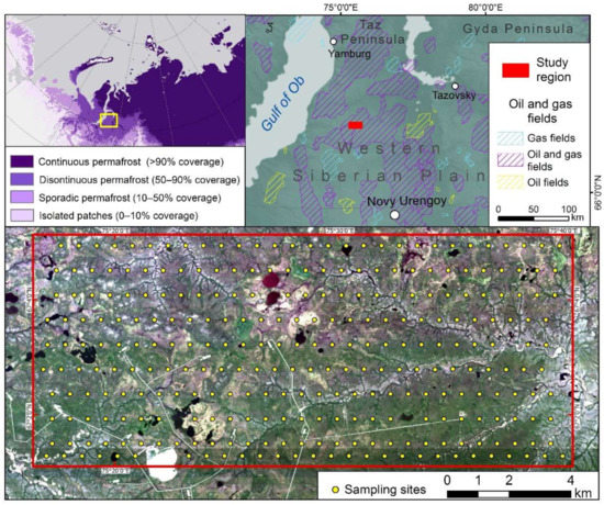
Figure 1.
Location of the study area within the permafrost zone (upper left) after Obu et al. [40] and on the map of hydrocarbon bearing fields (upper right), and location of the grid of sampling sites on the Sentinel image (bands 4, 3, 2).
Four structural elements of terrain occupied more than 99% of the study area, as follows:
- The Bakhta terrace (55–70 m a.s.l.), composed of marine and glacial-marine loams, loamy sands, and sands with pebble and gravel of Middle Pleistocene age (230–129 kyr).
- The Kazantsevo plain (55–60 m a.s.l.), represented by marine sands, loams, and loamy sands of Upper Pleistocene age (129–80 kyr).
- Alases (lacustrine and bog depressions formed by thermokarst) of Holocene age (younger than 11.7 kyr), forming gently sloping (slope classification according to [41]) plains (50–60 m a.s.l.), dominated by peats, silts, and loamy sands. Thermokarst lakes were mostly drained by shallow streams and converted to wetlands, but those remaining have depths of 2–5 m.
- Floodplains and terraces of rivers and gullies (40–50 m a.s.l.), composed of alluvial sands, diluvium, and proluvium of Holocene age.
The thickness of the Quaternary deposits varies from 70 to 200 m [42]. These are underlain by the following sediments within the interval of subzero temperatures down to depths as much as −400 m a.s.l. (Figure 2):
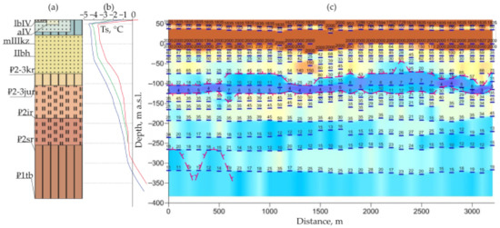
Figure 2.
Generalized geological section (a), including lbIV—modern lacustrine-boggy deposits, aIV—modern alluvium, mIIIkz—Kazantsevo formation, IIbh—Bakhta formation, ₽2–3kr—Korliki formation, ₽2–3jur—Yurki formation, ₽2ir—Irbit formation, ₽2sr—Serov formation, ₽1tb—Tibey-Sale formation. A detailed description is provided in the text. Permafrost temperature profile (b) in three boreholes drilled in the Pestsovoe gas field on oligotrophic fen (red) and polygonal peatlands with occasional (green) and dense (blue) ice wedges (TyumenNIIgiprogaz data). Shallow transient electromagnetic method (STEM)-based physico-geological model (c) of the study area to a depth of 400 m. Numbers indicate measured resistivity values (Ω∙m).
- i.
- Inequigranular sands, clays with the lenses of gravels, and interbeds of kaolinite of the Korliki formation of Upper Eocene-Oligocene age (37.8–23.03 Myr);
- ii.
- Clays and silts with interbeds of quartz-glauconite kaolinized sands, inclusions of gravels, and siderite concretions of the Yurki formation of Upper Eocene age (37.8–33.9 Myr);
- iii.
- Poorly defined diatomaceous earth and clays with interbeds of glauconite sands of the Irbit formation of Middle-Upper Eocene age (41.2–33.9 Myr);
- iv.
- Silica clays with interbeds of diatomaceous clays of the Serov formation of Lower Eocene age (56.0–47.8 Myr);
- v.
- Poorly defined silty clays with interbeds of sands and lenses of lignite of the Tibey-Sale formation of Paleocene age (66.0–56.0 Myr).
Tectonic maps show a regional fault with a W direction dissecting the study area, and linearly folded zones and fractures due to dynamic stresses in the N and NW directions [42].
Gas-, condensate-, and oil-bearing beds are found at several levels. The shallowest gas bed of Cenomanian age (100.5–93.9 Myr) at 1200 m below the surface has a thickness of 88 m and debits of 0.1–2.0 million m3 day−1. Oil and gas condensate from beds of Neocomian age (145–130 Myr) at depths of 2900–3200 m, with thickness of 20–80 m, is the main object of exploration. The fluid temperature reaches 85–90 °C and pressure is 30–34 MPa.
Although our study area falls into a zone of discontinuous permafrost on maps based on surface temperature modeling [40] (Figure 1), geological evidence [43], geothermal data, and our geophysical studies show that permafrost occurs continuously. Permafrost has a thickness of 300–400 m on the plains, and 150–250 m beneath rivers. Taliks down to depths of 2.5 m are common on drained uplands. Open taliks are reported for medium and large rivers and lakes having depths of more than 0.8 m and widths of more than 200 m [43]. Permafrost temperature at the depth of zero annual amplitudes (conventional depth where permafrost temperature is measured) ranges from −3.5 to −2.5 °C (Figure 2b) according to available data. Two layers of permafrost are divided by a layer of thawed sediments (talik) due to the partial permafrost degradation during the Early Holocene warming (10–5 kyr) and refreezing which started in the late Holocene (ca. 5 kyr) [44]. Seasonal thawing reaches 0.6–1.5 m in unconsolidated sediments, and could be as low as 0.3 m in peat. Seasonal freezing above taliks takes place down to 1.0–1.5 m. Average ground ice content of permafrost is 20%; however, deposits with high ice content exceeding 100% can be found in the topmost Quaternary part of the section [45]. Intrusive ice is found in the cores of pingos reaching 7 m in height and palsas, both widely present in the study area.
According to the Koppen-Geiger classification for 1980–2016, the study area has a regular boreal climate [46] with long (October–May), severely cold winters, with an air freezing index of −3734 degree-days and an average air temperature in January of −24.7 °C, and wet, cool summers with an average air temperature of 14.6 °C. The reported are the climate norms for 1988–2017 from Nyda (WMO 23245) and Tazovsky (WMO 23256) stations [47], weighted proportionally to the distance from the study area (200 and 245 km, respectively). Annual precipitation is 442 mm, of which 195 mm falls during summer. Precipitation occurs on an average of 172 days each year. Snow forms a cover with a thickness of 0.3–0.5 m on the plains, and up to 1 m in depressions from early October to late May, as measured by regular snow surveys in Tazovsky.
Landscapes are represented by different types of tundra, dominated by shrubs and grasses, with sparse alder groves and rare larch stands in the southern part of the study area or along the river valleys. The southern part of the study area neighbors the industrial infrastructure of the gas field; however, the impact of the latter on the landscape structure is limited to several unpaved roads [48].
2.2. Studies of Gas Composition in Frozen Soils
One type of petroleum geochemical survey is the study of the hydrocarbons absorbed by soil, which includes actually absorbed chemical compounds and the filling of the pore space [25]. The study area was split into latitudinal profiles with sampling sites located every 400 m. Profiles were located at a distance of 800 m from each other, forming a regular sampling grid on the study area (see Figure 1).
Coordinates of the sampling sites were uploaded to Garmin GPSMAP 60CSx (Garmin Ltd., Olathe, USA) with an average uncertainty of detection of ±10 m. Field technicians moved between the sites by snowmobile and/or skis, completed a standard form regarding the site description, and sampled frozen soils in February–March 2017. A total of 284 samples were collected.
On each site, a 0.7 m deep borehole was drilled with a hand auger, and the bottom 0.1 m of frozen soil (45–85 cm3) was sampled into 170 cm3 plastic containers. Containers with frozen soil were filled with 50–110 cm3 of saturated sodium chloride solution, preliminarily prepared from 99.999% NaCl powder in boiling water. Then, they were sealed with gas- and water-tight Teflon screw stoppers with butyl rubber centers, and were transported to the lab inverted. Teflon stoppers and tubing are widely used in soil gas and fluid sampling, and greenhouse gas measurement systems [49], because of their low permeability and diffusivity [50]. Although Teflon can leach carbon into the water [51], we do not expect this to have notably biased our gas samples because the area of contact with the stopper, which has an 18 mm diameter, is small. One month of sample storage and transportation to the lab at ambient winter temperature did not allow any notable amount of gas to be formed from the Teflon-derived carbon or diffused into the stopper.
Gases were extracted from the frozen soil using the headspace method [52] in a laboratory. Containers were placed in a water bath at a temperature of 60 °C, allowing the gas to escape to the headspace from the soil solution. The headspace was sampled by expulsion of the gas from the container to a syringe by creating excess pressure in the container with the addition of NaCl solution dispensed from another syringe. The volume of gas in the second syringe corresponding to the headspace volume (typically 15–30 cm3) was measured and subsampled for chromatographic analysis.
In addition to the CH4 and CO2, other gases and geochemical indicators that might indicate the geological origin of the gas mixture were studied. These included ethane (C2H6) and propane (C3H8), the most widespread components of natural gas after CH4, which can only scarcely be produced by natural soil microbiota, and have a lower diffusivity and longer time of decomposition than CH4 due to their larger molecules. These are conventionally used as indicators of hydrocarbon resources, both as the gas concentrations, and as part of the following indicators:
- C2+ C3 (the sum of C2H6 and C3H8, vol.%);
- C2/C3ratio (vol.% of C2H6 divided by C3H8) indicating leakage from either a gas or oil bed;
- C1/C2–3ratio (vol.% of CH4 divided by C2 + C3), indicating the cathagenetic (produced at high temperature from deeply metamorphosed organic matter in the rocks) or biogenic (produced microbially from organic compounds under surface conditions) origin of the gas mixture. C1/C2–3 ratio is above 1000 when the gas is biogenic, and is below 100 when it has migrated from a hydrocarbon reservoir [53].
To increase the efficacy of the lab, two chromatographs were used to find concentrations of CH4, C2H5, and C3H8 (hereinafter the variables of gas concentrations are denoted by the italicized chemical formula):
- A Chrom-5 (Laboratory Instruments, Prague, Czech Republic), equipped with a 3 mm × 3 m column filled with aluminum oxide, using helium as a carrier gas, and a flame-ionizing detector, with a quantification limit of 1 ppm;
- A Kristall-5000.2 (Chromatek, Yoshkar-Ola, Russia), equipped with a 0.25 mm × 100 m column filled with polydimethylsiloxane, using helium as a carrier gas, and a flame-ionizing detector, with a quantification limit of 0.4 ppm.
Chromatographs were calibrated using the standard gas mixtures. The sensor drift during the measurements was corrected by laboratory air sample testing.
Concentrations of carbon dioxide (CO2), helium (He), oxygen (O2), and hydrogen (H2) were measured with a gas chromatograph Gazochrom-2000 (Chromatek, Russia). This was equipped with two columns of 2 mm × 2 m HayeSep N and 2 mm × 3 m NaX, a thermal conductivity detector for incombustible gases, and a thermochemical detector for H2. Argon was used as a carrier gas.
Chromatographs used the standard gas mixtures to convert the electric signal from the detectors to volumetric concentrations of gases in the probe. The analysis and the outputs were controlled by the Chromatek Analysis software package (Chromatek, Russia). The concentrations were recalculated to the sample volume using the following equation:
where Ci is the volumetric concentration of gas i (cm3 of gas per m3 of frozen soil); CV is the volumetric concentration of gas in the headspace (ppmv); Vgas is the volume of gas extracted from the sample (cm3); and Vsoil is the volume of the soil sample in the container (m3). The volume of gas was then used to calculate its mass using the ideal gas law:
where mgas is the mass of gas (mg); Mgas is the molar mass of gas (g mol−1); 22,400 cm3 mol−1 is the standard volume occupied by 1 mol of ideal gas at standard conditions; p = 101,325 Pa is the standard pressure; T = 333.15 K = 60 °C is the temperature of the sample for chromatographic analysis; and R = 8.314 J K−1 mol−1 is the gas constant.
2.3. Studies of Subsurface Structure Using Geophysical Sounding
The structure of the upper part of the section was recognized in the eastern region of the study area using the shallow transient electromagnetic method (STEM)—measurements of electric and magnetic properties of sediments with an induced electromagnetic field. The induction in the sediments took place due to the periodical breaks of direct current from the generator in the transmitter loop of the coil on the surface. These breaks created the eddy currents and associated electromagnetic field in the sediments. The rate of dissipation of the field is physically linked to the resistivity of a sediment layer. Thicknesses of layers with different resistivities have been recognized [54,55]. Permafrost, compared to thawed sediments, has higher electrical resistivity because ice and unfrozen water disintegrate the mineral matrix, which is the preferential conductor of electric current.
Our STEM array had a rectangular receiver loop with side of 10 m inside of the rectangular transmitter loop with side of 100 m, thus forming an in-loop configuration [54]. The telemetric sounding system FastSnap (Sigma-Geo, Irkutsk, Russia) generated a block pulse of alternating current up to 20 A in the transmitter loop, which allowed sounding of a depth interval of 10–500 m below the surface with a resolution of 5 m. The array was moved along the profiles, creating a grid of measurements with 300 m spacings, i.e., a sampling density of ca. 16 points per 1 km2.
Resistivity data from every point were processed in the Model 3 software package (Sigma-Geo, Russia) [56], thus compiling the 3D geoelectric model of the study area [57]. The basis of the model was the etalon geoelectric section reconstructed from the geoelectric survey of a borehole that showed a typical section of the study area with full core description (Figure 2c). Several resistivity layers were recognized (top to bottom):
- The topmost 100–180 m had a resistivity up to 2000–3000 Ω m, associated with ice-bearing permafrost with ice content of 10–50% and a temperature from −2 to −5 °C;
- The 20 m thick layer below the permafrost had a resistivity of 5–10 Ω∙m which correlated to the thawed sands of an intrapermafrost talik;
- Down to depths of 350–400 m below the surface, there was a layer with a resistivity of 10–50 Ω∙m corresponding to cryotic (sediments at subzero temperature without ice) or thawed deposits.
High electric resistivity was a distinctive feature of the interval of ice-bearing permafrost. Because the non-icy cryotic sediments do not pose physical constraints on the migration of gases, their effect on gas migration through the permafrost was of less interest in our study. Variations of thickness of ice-bearing permafrost were used in our analysis of the effect of the subsurface structure on GHGs in the soil layer.
Analysis of gradient maps recalculated from the slices of resistivity at different depths allowed the zones of increased gradients of resistivity associated with faults or fractures to be recognized. Elongated objects with either an anomalously high or low resistivity were also interpreted as faults or fractures. The density of the fractures reaching the surface, i.e., length per unit area within the circle with a diameter of 450 m, centered on a sampling site, was used as a variable in our analysis.
2.4. GIS and Remote Sensing Studies
We created a geodatabase (GDB) in a GIS environment, based on field geochemistry and geophysical data, geological maps, and remote sensing data. The compiled GDB contains 30 descriptive attributes for each sample site (Table A1). The GDB was projected to the Universal Transverse Mercator Zone 43N coordinate system using the World Geodetic System 84 ellipsoid datum. Georeferencing and digitizing of maps, lineament analysis, overlay operations, mapping of density of linear features, and extraction of values from vector and raster data were carried out using ArcGIS 10.4 (ESRI, Redmond, WA, USA). Remote sensing data and maps were used to reveal land surface variables, which control CH4 and CO2 storage in frozen soils. The GDB was the key component of our factor study and regional assessment of winter stocks of GHGs in soils.
2.4.1. Terrain and Geological Data
A digital elevation model (DEM) of the study area was a subset from the high-resolution ArcticDEM model created from WorldView-1/2/3 and GeoEye-1 satellites covering lands north of 60° N [58]. The mosaicked 2 m resolution DEM file of the Polar Geospatial Center Release 7 was used. Absolute heights, aspect, and slope data for each sample field site were derived based on the analysis of the DEM.
Thematic plates of the state geological map at the 1:200,000 scale [42], including tectonics, Quaternary deposits, and Pre-Quaternary deposit plates, were georeferenced and digitized. These data were combined with the DEM to compile the geomorphology map of the study area.
2.4.2. Lineament Analysis
A lineament is a linear surficial feature, sized and oriented in association with an underlying tectonic structure—a joint or a fault [59]. We performed the visual lineament allocation and interpretation routine, which allowed higher quality compared to using software for automatized lineament detection. We used Sentinel-2 images of 10 m resolution (30 July 2019) and ArcticDEM of 2 m resolution to allocate the elementary lineaments at the 1:30,000 scale. All straight lines on the surface, associated with erosion, river networks, and lake shores, were interpreted as elementary lineaments. Image analysis for lineament detection was performed using several band combinations such as natural color (bands 4, 3, 2), color infrared (bands 8, 4, 3), and geology (bands 14, 4, 2). In addition, we allocated lineaments at a 1:100,000 scale from Sentinel-2 and ArcticDEM. Finally, we repeated the detection process using the DEM at a 1:200,000 scale. This stepwise scaling allowed both the elementary and generalized lineament systems to be allocated.
Taking into account the uncertainties associated with mapping and GPS, we assumed that a lineament has a buffer zone of 30, 100, or 200 m corresponding to the scale at which it is recognized (1:30,000, 1:100,000, and 1:200,000, respectively). If a sampling site fit into the buffer zone, it was attributed with its smallest size. Moreover, the density of lineaments was calculated similarly to the density of the faults.
2.4.3. Land Cover
We used land cover classification from Sentinel-2 and Sentinel-1 for West Siberia [48]. The classification was performed using a combined approach of supervised and unsupervised classification based on optical Sentinel-2 band 3 (green, 10 m), 4 (red, 10 m), 8 (near infrared, 10 m) 11 (short-wave infrared (SWIR) 20 m), and 12 (SWIR, 20 m) and radar Sentinel-1 VV (interferometric wide swath). The land cover map of 20 m resolution was based on 21 classes that belong to several land cover groups: Sparse vegetation, Shrub tundra, Forest, Grassland, Floodplain, Barren land, and Water. Most land classes are characterized by moisture content, which we used as a separate attribute in our analysis. A full list of the landscape classes is given in Table A2.
2.5. Geostatistics
Statistical analysis of the GDB was conducted to find links between GHG concentrations in frozen soils with surface and structural variables (Table A1), in addition to finding any manifestations of subsurface structures in surface features. The links between the surface factors are not shown and not discussed in this study.
Regression analysis was carried out with the R software package [60]. One of the main conditions imposed on the regression analysis was the normality of the variables. The variables were tested for normality and normalized when needed. Normalization functions (see Table A1) were found with the powerTransform function from the car package.
Links of dependent variables CH4 and CO2 with other factors were estimated using multiple linear regression without interaction of variables. The most significant independent variables were identified using the function regsubset from the leaps package.
The null hypothesis implies there is no link between the variables. The significance of the link was tested with the Z-test and characterized with the probability value (p-value). At p < 0.1, the null hypothesis was rejected, and the p-value was used to demonstrate the significance of the link. All values reported in Section 3 and Section 4 were derived from the means ± standard deviations of normalized datasets.
3. Results
3.1. Variability of GHGs and Other Gases in Frozen Soils
The maps of CH4 and CO2 in frozen soils are shown in Figure 3. There was 0.016 (0.005-0.062) g CH4 m−3 soil. CH4 had localized spots of anomalously high concentrations above 0.1 g m−3 in the eastern region of the study area, and was more concentrated and robust in the SW (Figure 3a). CO2 tended to be inversely linked to CH4 (p < 0.1). CO2 was three orders of magnitude more abundant, i.e., 11.439 (4.888–22.507) g m−3 soil. Its lows of below 5 g m−3 formed elongated patches oriented to the northeast in the central and eastern regions of the study area. Anomalously high CO2 above 40 g m−3 formed dense north and northwest oriented patches tending to the western region of the study area (Figure 3b).
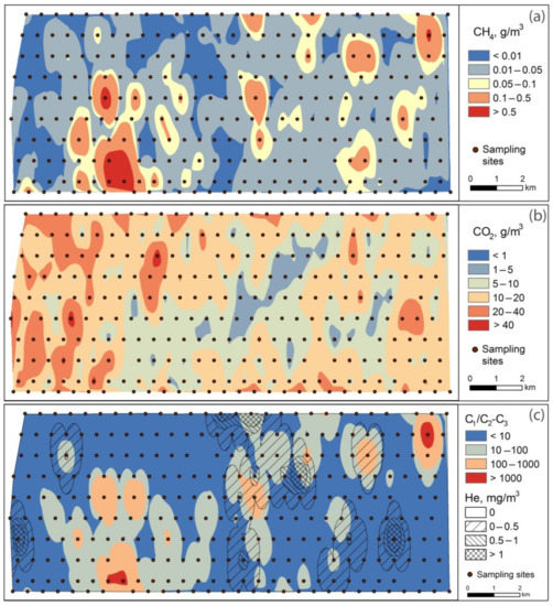
Figure 3.
Concentrations of gases and geochemical indicators at depths of 0.6–0.7 m in frozen soil on a hydrocarbon field of the study area in winter 2017: (a) CH4, (b) CO2, and (c) He and C1/C2–3 ratio.
The full set of variables described 52.19% of the variations of CH4 and 36.12% of the variations of CO2 (both at p < 0.001). CH4 had direct links with C3H8, H2, and C2H6 (all at p < 0.001), and an inverse link with O2 (p < 0.01). C2H6 was 0.002 (0.0003–0.010) g m−3, and C3H8 was 0.004 (0.001–0.010) g m−3, so that the C1/C2–3 ratio was below 10 on 94% of the study sites. Anomalies of C1/C2–3 ratio coincided with anomalies of CH4 (p < 0.05), but were driven mainly by C3H8 (r = 0.98). He was 0.001 (0.0002–0.002) g m−3 in 16 study sites (Figure 3c). Several anomalies of CH4 tended to collocate with He (p < 0.1), although in most cases CH4 was 0.021 (0.008–0.064) g m−3, i.e., only 0.005 g m−3 above the background in sites where He was above zero. There were 0.005 (0.001–0.118) g H2 m−3 and 64.365 (30.789–110.183) g O2 m−3. CO2 was linked with O2 (p < 0.001) and had a less significant link with C3H8 (p < 0.05).
3.2. Thickness of Permafrost and Faults Reaching the Surface
Permafrost thickness (variables are hereinafter italicized) within the study area was 132 m, and varied from 107 to 157 m (Figure 4a). It was directly linked with Altitude (p < 0.001), Latitude, and Longitude (both p < 0.01). Permafrost thickness significantly differed across Morphology: 135 (123–147) m on Bakhta terrace (IIbh, see sediment description in Section 2.1 and on Figure 2), 130 (128–155) m on Kazantsev marine terrace (mIIIkz, both at p < 0.01), 151 (128–174) m within alases (lbIV, p < 0.05), and only 127 (118–136) m on floodplains (aIV). Permafrost progressively thinned with Slope class (p < 0.01), being 139 (112–166) m under flat to nearly level slopes and 125 (104–146) m under very gentle to regular slopes. It tended to be slightly thicker, at 137 (112–162) m, under northwestern, southeastern, northern, and southern slopes than under northeastern, southwestern, eastern, and western slopes (128 (104–152) m, p < 0.1).
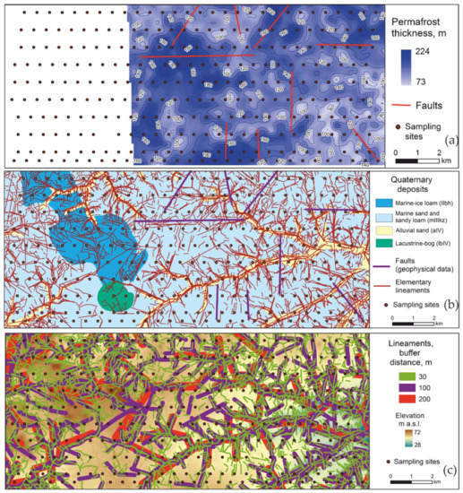
Figure 4.
Maps of structural features tested for an effect on gas concentration in frozen soils: (a) Permafrost thickness and faults reaching the surface based on shallow TEM data; (b) faults and lineaments across sediment types (see details of geological indexes on Figure 2, and sediment description in Section 2.1) and elements of terrain; and (c) Lineament buffer distance distribution.
Permafrost thickness increased along the gradient of wetness in landscapes dominated by dwarf shrubs and grasses, from 110 (100–120) m in moist low-density shrubs, to 149 (124–174) m in dry to moist prostrate shrubs (p < 0.05). Overall, 44% of variations of Permafrost thickness were sufficiently described by our dataset (p < 0.001).
Faults that were recognized geophysically tended to occur in areas with thicker permafrost (p < 0.1). Nine joints/faults reached the surface. These dissected slopes of watersheds and had northern, northeastern, eastern, and rarely southeastern orientation (Figure 4a). Faults density was sparse at 0.247 (0–0.686) km·km−2. Faults were the most pronounced in peats and this abundance decreased with soil grain size, with a maximum in areas laid with peaty sands 0.465 (0–0.985) km·km−2 and a minimum of 0.197 (0–0.589) km·km−2 in loamy deposits (p < 0.05). Faults density grew from 0.822 (0.442–1.202) km·km−2 in the vicinities of sites located on flats to very gentle slopes, to 0.974 (0.543–1.405) km·km−2 on gentle to regular slopes (p < 0.05). It tended to be higher in the vicinities of sites located on northeastern, eastern, and southern slopes (p < 0.1).
Lineaments formed a dense network of 9.306 (4.802–13.810) km·km−2 in the study area (Figure 4b). It was only in rare cases in the north-central area that they followed the faults network; however, in general, they did not coincide (p = 0.38). Lineaments of northwestern-southeastern and western-eastern orientation dominated (Figure 4c). A total of 57.27% of variations of Lineaments density was described (p < 0.001) by Altitude (p < 0.001) and Landscape (p < 0.05). Dry to moist prostrate to erect dwarf shrub tundra had significantly less (p < 0.01) lineaments of 6.644 (2.058–11.228) km·km−2. Similar to the faults, Lineaments density was highest in sands; conversely, it was lowest in peats, and always lower in peaty soils than in mineral. It tended to decrease with grain size from 10.854 (6.320–15.388) km·km−2 in sands to 8.453 (4.785–12.121) km·km−2 in loams (p < 0.1). As shown in Figure 4b, Lineaments density significantly differed between Morphological elements of terrain (p < 0.01), reaching the maximum of 16.203 (12.267–20.140) km·km−2 on floodplains, and the minimum of 6.497 (3.475–9.520) km·km−2 in alases.
Lineaments density grew with the distance of sampling sites from the nearest lineament, i.e., Lineament buffer (p < 0.01). Lineament buffer was linked with levelled slopes (p < 0.01), peaty loamy sands (p < 0.05), and northwestern slopes (p < 0.05), and Graminoid, prostrate dwarf shrub, patterned grounds, and partially bare Land cover classes.
Proximity of a fault did not have an effect on gas concentration in soil. However, CH4 grew closer to lineaments: within 30 m of a lineament there was 0.020 (0.006–0.081) g m−3, compared to 0.014 (0.005–0.048) g m−3 in the 200 m buffer (p < 0.05). None of the structural variables were linked to CO2. He tended to decrease with Permafrost thickness, where it was above zero (p < 0.1, n = 16). Permafrost tended to be slightly thicker, at 133 (108–158) m, for sites with no He in the soil than for sites with He (p < 0.1), where it was 125 (102–148) m. Permafrost thickness tended to grow with C1/C2–3 ratio from 129 (105–153) m for sites with values <10 to 168 (149–187) m for sites with values above 100 (p < 0.1).
3.3. Surface Factors of the GHG Concentrations in Soils
Surface controls are the complex of factors affecting production, transformation, and exchange of gas in the active layer (Table A1). GHGs significantly differed across Land cover types and Land cover groups (both p < 0.05); see Table 1, Figure 5. Peaks were found in the Forest group, in which Shrub tundra mean values were exceeded by a factor of 4 for CH4 and by 1.5 for CO2. The combined Floodplains and Water groups had slightly lower concentrations of GHG than Shrub tundra. The Sparse vegetation group was the second highest for CH4, and the lowest for CO2. GHG concentrations differed across the diversity of land cover classes of the most widespread Shrub tundra group. The highest CH4 was found in Moist to wet graminoid prostrate to erect dwarf shrub tundra. The lowest CH4 and the highest CO2 occurred in Moist low-density shrubs. The minimum of CO2 was found in Dry to moist prostrate to erect dwarf shrub tundra.

Table 1.
Variations of CO2 and CH4 with Land cover class and Morphology, serving the bases for upscaling in estimates of the storage of greenhouse gases (GHGs) in frozen soils.
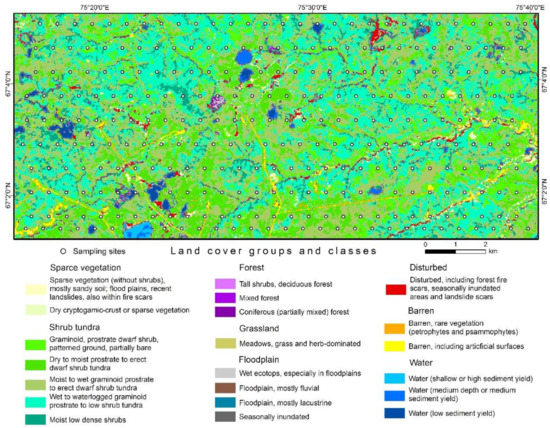
Figure 5.
Land cover groups and classes in the study area. Adapted with the permission from ref. [48], 2019, A. Bartsch, B. Widhalm, G. Pointner, K. Ermokhina, M. Leibman, B. Heim.
On the other hand, the Morphology of terrain tended to control GHGs (see Table 1) (p < 0.1). The watersheds had higher CO2 and lower CH4 than depressions. Floodplains and bottoms of gullies had the lowest GHG concentrations.
GHG concentrations significantly differed with Aspect (p < 0.05) and tended to be sensitive to Slope (p < 0.1). CH4 had a maximum of 0.029 (0.007–0.161) g m−3 on flats, and the second highest value of 0.020 (0.006–0.081) g m−3 on moderate slopes. CO2 gradually decreased with Slope steepness from 12,555 (6.170–22.541) g m−3 on flats, to 7.603 (5.927–9.586) g m−3 on moderate slopes. The lowest CH4 of 0.014 (0.004–0.056) g m−3 was found on southeastern and northwestern slopes, whereas the highest CH4 of 0.019 (0.005–0.084) g m−3 occurred on northern slopes. On the contrary, the highest CO2 of 13.276 (5.436–26.829) g m−3 was found on northwestern slopes, and the lowest of 9.470 (4.341–17.810) g m−3 on southwestern slopes. Variations of GHGs in all other Aspects did not differ significantly.
Moisture characteristics based on Land cover classes (Table A2) did not show any significant links with either the concentration of gases in frozen soils or the variables of the subsurface structure.
Statistical analysis showed CO2 increased with Latitude (p < 0.01); however, no correlation was found (r = 0.05).
4. Discussion
GHGs in frozen soils may have been produced biologically from organic matter in the soil due to multiple surface factors that control the production, transformation, and migration [4]. Alternatively, CH4, C2H6, and C3H8, which act as precursors of CO2 [61,62], may have migrated to the soils with fluids from a geological source located within or below the permafrost layers. The origin of GHGs can be deduced from geochemical ratios and distribution patterns of C2H6, C3H8, He, and H2. Our evidence suggests that contribution of gases from both sources was likely (Figure 6). In the Subsections below we discuss the nature of the links and the share of the geological sources in the soil gas pool of the oil and gas field.
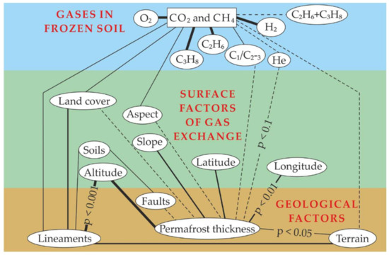
Figure 6.
Links between geological and surface factors of gas composition in frozen soils. Thickness of a line indicates the significance of the link: thickest—p < 0.001, medium—p < 0.01, hairline—p < 0.05, and tendencies with p < 0.1.
4.1. Geological Sources
The most likely geological source of GHGs in an oil and gas field are hydrocarbon enriched beds lying at depth below the ice-bonded permafrost base. At the same time, we cannot exclude the showings of subsurface volcanism or hydrothermal sources [5,6,16,17]. Following F.E. Are [13], and given the low permeability of permafrost, we searched for linear anomalies of CH4 and CO2 and markers of fluid migration (C2H6, C3H8, H2, and He) along the faults, recognized with STEM and lineament analysis.
On the other hand, fluids always filtered through the thawed sediments before permafrost formation and they had enriched the sediments by the time of Holocene freezing [22]. Nowadays, the disperse gas filling the pores, gas accumulations, or gas hydrates in permafrost form a diffusion flow to the soils, which is catalyzed by permafrost degradation.
4.1.1. The Effect of Tectonics on Fluid Shows in Soils
Faults density and Lineaments density had no links to the concentration of GHGs. Surprisingly, the faults recognized with STEM were not related to lineaments. They tended to be denser on thicker permafrost (Figure 4a), and located within the watersheds (Figure 4b), i.e., in the inner parts of tectonic blocks. Hence, they are likely inactive dislocations which do not reach the permafrost base and could not serve the channels for migration gases.
GHG concentrations had a direct link with only one of the geological factors (Figure 6), the Lineament buffers. The Lineaments density found on floodplains exceeded, by two to three orders of magnitude, that of other Terrains. Floodplains had the lowest Permafrost thickness, associated with higher heat flow below the streams flowing along the tectonic joints, which serve as the preferable path for fluid migration.
A significant link of CH4 with Lineament buffers indicates that CH4 itself might be associated with geological sources that are more active in the vicinities of lineaments. A first-order estimate of the contribution of geologic CH4 (CH4–geo) from the active joints to CH4 in frozen soils, based on the assumption that proximity to the lineament is the predictor, was derived with the best-guess function (R2 = 0.946), as follows:
Within 0.1 m of a lineament, the CH4 would be 0.062 g m−3, including 0.047 g m−3 from geological sources and 0.013 g m−3 of background soil microbial CH4, the average for the areas outside the Lineament buffers (see Section 4.2).
Nevertheless, the gas composition along the lineaments did not differ significantly from the background, except that the linear links between CH4 and C2H6, C3H8, and H2strengthened with proximity to lineaments to medium r values of 0.48, 0.63, and 0.52 (n = 160), respectively, in Shrub tundra, the most widespread land cover group. Conversely, the linear link between CO2 and C3H8 reached a medium r = 0.50 outside of the 200 m buffer zone around lineaments (n = 101), which will be discussed in Section 4.1.3. Similar strengthening of the links was noted for other Land cover types with characteristic different Moisture, a control on the GHG production/oxidation processes. Hence, the changes in the way the concentrations of hydrocarbons vary close to lineaments show that gas migration runs differently than outside. Even though H2 could be produced and consumed in soil [63], we consider the fact of the strengthening of the links between gases as indicators of the higher activity of geological sources which contributed to CH4 around the lineaments.
In future studies, it will be important to search for and sample CH4 anomalies along lineaments in localities of their highest density, i.e., river valleys and bottoms of gullies, which have earlier been reported to have high CH4 [64,65]. An analysis of stable isotopes may provide better indications of their genetic linkages.
4.1.2. Microseeps
Sporadic anomalies of He, a gas of mantle origin [13,25], occurred at 5% of the study sites. They usually had a concentric core with He of above 0.0005 g m−3 surrounded with an aureole of lower He, forming a circular anomaly with a diameter of ca. 1 km (Figure 3c). Although the superposition of Figure 3c on Figure 4a,c shows that the anomalies often lie in vicinities of fault endings and centers of increased lineament density, there were no statistically significant linkages found between He and structural elements. Given the form of the anomalies and high migration capabilities of He, it is more likely that the constant flow existed in the centers of anomalies than that a sudden He efflux was entrapped in the soil. This implies occurrence of a microseep, a channel of fluid migration through permafrost projected as a point source to the soil profile.
None of the gases had significantly different concentrations within the He anomalies, with the exception of 0.005 g m−3 higher CH4 (p < 0.1), which might be taken as a first-order estimate of the geologic contribution to the soil CH4 on microseeps.
Until specific studies of microseeps in the permafrost zone are conducted, we can only speculate that the traps for gases physically form with soil freezing [66], and that such microseeps are connected with hydrocarbon bearing reservoirs. The chemical or biological transformation of hydrocarbons during microseep migration, or in the soil, might not necessarily have been reflected in the selected geochemical indicators or under our study design.
4.1.3. Diffuse Flow
When the migration channels are small and distributed to a series of tortuous pathways where gas flows through the pores, the fluid migration is better described with the diffuse flow. It forms the vast distributed anomalies of hydrocarbons of geological origin on our study area (Figure 3c). We assume hydrocarbons as an indicator of the diffuse flow as there is limited production and accumulation of these gases in soil [67]. The fact that C3H8 and C2H6 were of the same order with CH4 at most of the sites implies low probability that hydrocarbons were produced in the soil. C2H6 and C3H8 had similar distribution patterns across the study area. Had they originated from contamination, we would have found the anomalies in the proximity of extraction sites and exploration infrastructure in the southern part of the study area (compare Figure 3c and the Barren, including artificial surfaces Landcover class in Figure 5). The significant link of CH4 with hydrocarbons could evidence the mutual participation in the fluid flow.
CH4 made the largest contribution to maintain the C1/C2–3 ratio below 100 units in the majority of sites (n = 269; Figure 7). The same order of C2 + C3 across all areas supports the idea of quite similar and constant diffusion flow from hydrocarbon beds in the study area. CH4 rich sites depleted in C2 + C3 (Figure 6 and Figure 7) coincide with the alases Terrain, which stood out from the background C1/C2–3 ratio with the average of 172 units, and the maximum of 467 (n = 16). Alases in the study area have thick permafrost, which could have prevented the penetration of deep fluids. It is a surprising fact, because evidence from Alaska showed that a thermokarst lake, a precursor of an alas, is a weak zone providing the fluid migration through permafrost [17]. This fact emphasizes regional geological differences in that the stronger biogenic production in alases has likely hindered the diffuse flow through West Siberian permafrost, but it could not perform the 3 orders of magnitude stronger Alaskan seeps. The diffuse flow through permafrost should be less than the migration flow of microseeps, so the 0.005 g CH4 m−3 could be taken as a first-order upper estimate of the diffuse flow.
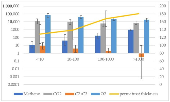
Figure 7.
Changes in concentrations of greenhouse gases, hydrocarbons (g m−3, left axis), and permafrost thickness (m, right axis).
Laboratory incubations have shown that the half-life of C3H8 in soils of different wetness and composition at temperatures of 1–3 °C is 20–100 h, during which the concentration decreases exponentially to trace values [68]. Hence, hydrocarbon concentrations in freezing soils of our site should have degraded to trace amounts at the minimum rate in the timeframe of several days without a sourcing flow. Data from the Circumpolar Active Layer Monitoring site R50b [69] lying 50 km north of our study area showed the average thaw depth of 0.93 cm in 2017 froze over the duration of 1 month [70]. Over the course of complete freezing of a soil profile, around 1 g m−3 of C3H8 would have been degraded, i.e., 250 times more than the maximum value we found in the study area. For sites with peaty soils comprising 2% of the 0.01 km2 plot at the R50b [69], the thaw depth was less than 0.7 m. Thus, it is likely that in peatland soils we have sampled the permafrost. Even in this case, the difference in concentrations of hydrocarbons between peat and other Soil types in our study area was insignificant.
These two facts make us sure that the diffuse flow of hydrocarbons, including the CH4, was formed by continuous fluid migration through permafrost and was not just limited to secondary migration of gases from degrading permafrost enriched with hydrocarbons [22].
Links between CO2 and hydrocarbons could show the biodegradation of hydrocarbon-containing fluids in the soil profile. The production of GHGs from substrates associated with hydrocarbon degradation is a stepwise process involving multiple reactions [61] with acetic acid as one of sub-terminal products and CO2 as a terminal product. However, there are too few data on this matter to produce quantitative estimates.
Emission chamber and soil gas probe studies as well as experimental data on the microbial transformation of hydrocarbons should be undertaken to understand the balance of hydrocarbons and GHGs in soils and permafrost.
4.2. Contribution of Geological and Surface Factors to Concentration of GHGs in Frozen Soil
The effects of surface factors on the pool of GHGs in the soils were mediated by the Land cover class, which combine both vegetation and moisture conditions of a site. Although the non-validated classification has blurred the patterns of individual Land cover classes, the strongest links have been traced. CO2 grew across Domains from Sparse vegetation to Forested sites (Table 1), obviously following the increase of higher litter inputs to soils from higher phytomass [26]. CH4 showed significant difference reaching high values on the Disturbed sites.
Terrain types which served as a topographical characteristic tended to have an effect on GHGs. Floodplains and gullies as well as water bodies tended to have lower GHG concentrations. Alases had two times higher CH4 than the study area average, reflecting the favorable regime for methanogenesis characterized with high organic content and soil wetness [71].
If CH4 and CO2 were liberated from frozen soils to the air due to seasonal thawing, the flux would be equal to the total estimate of the pool as shown in Table 1, i.e., around 11.44 g m−2 CO2 and 0.02 g m−2 CH4. This is the only proxy for the winter pool of GHGs in frozen soils available up to date. These numbers fall within the range of the winter GHG fluxes reported in other studies [1,2,3,28,31,34,35,36,37,38,39]. Our estimate includes both the geogenic and biogenic components and does not make the oil and gas field area stand out from the naturally occurring values.
In Table 2 we have summarized data on the effect of the fluid migration on the study area to deduce the role of the geological and surface factors. A quite high CH4 storage, which appears along the buffers, exceeds the minimum estimate of the total storage of the study area (Table 1). The total quantifiable contribution of CH4 from geological sources is roughly one-half of the average estimate, or 15% of the maximum CH4 storage in the study area.
Table 2.
Summary of the effect of different geological sources on CH4 in frozen soils of the study area.
Because of the high uncertainties in the rate of C3H8 and CH4 oxidation in frozen soils, we cannot quantify the geological contribution to carbon dioxide. However, we surely have no reason to underestimate the role of surface factors. O2 could serve as an indicator of surface factors’ effect on the production of GHGs. The level of aeration of the soil profile measured by O2 indicates aerobic/anaerobic conditions controlling the pathway of organic matter decomposition and dominant CO2 or CH4 production, respectively [3,28]. Unsurprisingly, medium (r = 0.3–0.7) to strong correlations (r > 0.7) exist between CO2 and O2 across land cover classes in the most representative Domain of Shrub tundra, with maximum correlations in shrub dominated classes. We can conclude that the contribution of surface factors to GHGs production is ubiquitous.
We compared our estimate of the storage of carbon in the form of GHGs in frozen soil of 3.13 (1.34–6.19) g C m−3 of soil (recalculated from Table 1 using molecular masses of CO2 (44 a.m.u.), CH4 (16 a.m.u.), and C (12 a.m.u.)) with the concentration of carbon of SOM in the topmost meter of permafrost of 7.9–69.1 kg C m−3 (recalculated from storage density in kg C m−2 within 1 m of soil [72]). The storage of GHGs in frozen soil during winter was approximately 0.01–0.1% of the total carbon of SOM. Its contribution is low. It must be noted that this is a conservative estimate due to the leaks that might have taken place from this soil horizon after freezing due to cryogenic processes and plant-mediated transport. Secondly, the contribution of geological flow to CH4 and CO2 concentration in the frozen soils of 95% of the area marked with high concentrations of hydrocarbons cannot be assessed without knowledge of the microbial processes of the biodegradation of hydrocarbons and methane oxidation. Additional laboratory tests are needed to measure these rates. Additionally, the gaseous or dissolved form of a GHG in the frozen soils makes it more volatile, i.e., reactive, than SOM. We believe that these substances might be an easily consumable form of carbon preserved by the Arctic ecosystem to boost production when soil begins to thaw, acting as a soil fertilizer and catalyzer of growth of a number of microorganisms.
5. Conclusions
GIS-based statistical analysis of geochemical, geological, geophysical, morphometric, and land cover variables revealed the effects of fluid flow controlled by subsurface structure and surface factors controlling biogenic greenhouse gas production in soils on the concentrations of CO2 and CH4 in frozen soils. Our study demonstrates the dominance of soil production of these gases even on an oil and gas field. Nevertheless, fluid flow sourced either from hydrocarbon beds or secondary accumulations in permafrost could have contributed 15–50% of the CH4 observed in the frozen soil.
Hydrocarbons, C2H5, and C3H8 had concentrations of an order of magnitude similar to that of CH4, although they are not typically produced in soils, so the C1/C2–3 ratio indicated the geological origin of gas in 93% of the sampling sites of our 130 km2 study area. However, the power of this source cannot be reliably estimated.
Tectonic joints and the areas around them, marked with streams and rivers, served as the main conduit for geological CH4 flow.
Helium anomalies indicating microseeps occupied 5% of the study area. However, they were the source of only slightly higher methane concentrations.
The effect of permafrost thickness on GHG concentrations in the soil is indirect. Thick permafrost limited the flow of the hydrocarbons. It was more penetrable around the lineaments and seeps under a higher flux. However, in most cases it retained the diffuse flow of fluids.
The contribution of greenhouse gases from geological sources to their concentration in frozen soils can be deduced with studies of the patterns of the concentrations in soil profiles. We only tested one depth in the soil profile that made a negligible contribution to the soil carbon pool, of 0.01–0.1% of the typical carbon content of soil organic matter, not the whole profile. This overwintering soil pool is likely to be higher because, according to other studies, the comparable amount is discharged during freezing. This could act as a fertilizer and catalyzer of microbial biomass upon soil thawing, and has not yet been taken into account by any of the known models of carbon balance in the Arctic.
Author Contributions
Conceptualization, G.K. and A.B.; methodology, G.K., A.B., A.V. and V.G.; software, A.V., V.G. and I.S.; validation, G.K., A.B., A.V. and V.G.; formal analysis, G.K., A.B., A.V., S.S., V.G. and I.S.; investigation, G.K., A.B., S.S., I.S.; resources, A.B., A.V., V.G., I.S. and S.S.; data curation, G.K., A.V. and S.S.; writing—original draft preparation, G.K., A.B., A.V., V.G. and I.S.; writing—review and editing, all authors; visualization, G.K., A.B., A.V., I.S. and S.S.; supervision, G.K. and A.S.; project administration, G.K., A.B. and A.S.; funding acquisition, G.K., A.B. and A.S. All authors have read and agreed to the published version of the manuscript.
Funding
This study was supported by the RUSSIAN SCIENCE FOUNDATION, grant number 19-77-10065.
Acknowledgments
The authors thank M.D. Zavatskii, head of the chemical laboratory at Tyumen Industrial University, for chromatography analyses and the anonymous reviewers for their constructive remarks which helped to significantly improve the manuscript.
Conflicts of Interest
The authors declare no conflict of interest. The funders had no role in the design of the study; in the collection, analyses, or interpretation of data; in the writing of the manuscript; or in the decision to publish the results.
Appendix A. Variables Used in the Geodatabase and Statistical Analysis
Table A1.
List of variables of the geodatabase used in this study with normalization functions used in statistical analysis.
Table A1.
List of variables of the geodatabase used in this study with normalization functions used in statistical analysis.
| Variable | Description | Normalization Function |
|---|---|---|
| Site ID | Field number of the sampling site | |
| Concentrations of gases in frozen soils | ||
| CH4 | Concentration of methane in frozen soil at 0.6–0.7 m depth, mg m−3 | =CH4−0.1236 |
| C2H6 | Concentration of ethane in frozen soil at 0.6–0.7 m depth, mg m−3 | =C2H60.14 |
| C3H8 | Concentration of propane in frozen soil at 0.6–0.7 m depth, mg m−3 | =C3H80.13 |
| C2 + C3 | Sum of concentrations of ethane and propane in frozen soil at 0.6–0.7 m depth, vol.% | |
| C1/C2–3 ratio | Ratio of volumetric concentration of gases in frozen soil at 0.6–0.7 m depth, measured in vol.%, units | |
| C2/C3 | Ratio of volumetric concentrations of ethane to propane in frozen soil at 0.6–0.7 m depth, measured in vol.%, units | |
| CO2 | Concentration of carbon dioxide in frozen soil at 0.6–0.7 m depth, mg m−3 | =CO20.3 |
| O2 | Concentration of oxygen in frozen soil at 0.6–0.7 m depth, mg m−3 | =O20.5 |
| H2 | Concentration of hydrogen in frozen soil at 0.6–0.7 m depth, mg m−3 | =H20.25 |
| He | Concentration of helium in frozen soil at 0.6–0.7 m depth, mg m−3 | |
| Surface factors | ||
| Lat. | Latitude, ° N | |
| Lon. | Longitude, ° E | |
| Soil | Soil class based on grain size and organic matter content based on Russian classification [69] | |
| Alt. | Altitude, based on DEM, m | =alt2 |
| Slope | Slope, based on DEM, ° | =slope0.11 |
| Slope class | Slope class, following the Food and Agriculture Organization [41] classification | |
| Aspect | Vector of a slope, ° | =aspect0.5 |
| Orientation | Direction which slopes face, the classes of aspect, based on the 16-wind compass rose | |
| Land cover type no. | Code of land cover type following A. Bartsch et al. [48] classification (Table A2) | |
| Land cover type name | Class name of the land cover type following A. Bartsch et al. [48] classification (Table A2) | |
| Domain | Group of the land cover types following A. Bartsch et al. [48] classification (Table A2) | |
| Wetness | Dry, moist, wet, or waterlogged land classes following A. Bartsch et al. [48] classification (Table A2) | |
| Geological factors | ||
| Terrain | Surface morphological feature characterized by the altitude and the type and age of sediments composing it, based on DEM data and geological map [42] | |
| Lineament buffer | Distance to the nearest lineament from the sampling site, three categories corresponding to lineaments detected at different scales: 1:30,000 scale—30 m buffer distance; 1:100,000 scale—100 m buffer distance; 1:200,000 scale—200 m buffer distance; and a category of NOT APPLICABLE for all others | |
| Faults density | Length of the gradient zones reaching the surface using an electric survey in a circular neighborhood with a diameter of 450 m around the sampling site, km·km−2 | |
| Lineaments density | Length of lineaments in a circular neighborhood with a diameter of 450 m around the sampling site, km·km−2 | |
| Permafrost thickness | Thickness of the topmost interval with the electric resistivity corresponding to various ice-containing sediments, m | |
Table A2.
Data codes for the land cover product. Adapted from ref. [48]. CC-BY-4.0, © 2022. A. Bartsch, B. Widhalm, G. Pointner, K. Ermokhina, M. Leibman, B. Heim.
Table A2.
Data codes for the land cover product. Adapted from ref. [48]. CC-BY-4.0, © 2022. A. Bartsch, B. Widhalm, G. Pointner, K. Ermokhina, M. Leibman, B. Heim.
| Data Code (No.) | Class Name | Group | Wetness |
|---|---|---|---|
| 1 | Sparse vegetation (without shrubs), mostly sandy soil; flood plains, recent landslides, also within fire scars | Sparse vegetation | No data |
| 2 | Dry cryptogamic-crust or sparse vegetation | Sparse vegetation | Dry |
| 3 | Graminoid, prostrate dwarf shrub, patterned ground, partially bare | Shrub tundra | No data |
| 4 | Dry to moist prostrate to erect dwarf shrub tundra | Shrub tundra | Dry to moist |
| 5 | Moist to wet graminoid prostrate to erect dwarf shrub tundra | Shrub tundra | Moist to wet |
| 6 | Wet to waterlogged graminoid prostrate to low shrub tundra | Shrub tundra | Wet to waterlogged |
| 7 | Moist low-density shrubs | Shrub tundra | Moist |
| 8 | Tall shrubs, deciduous forest | Forest | No data |
| 9 | Mixed forest | Forest | No data |
| 10 | Coniferous (partially mixed) forest | Forest | No data |
| 11 | Meadows, grass and herb-dominated | Grassland | No data |
| 12 | Wet ecotops, especially in floodplains | Floodplain | Wet |
| 13 | Disturbed: seasonally inundated areas and landslide scars | Disturbed | No data |
| 14 | Floodplain, mostly fluvial | Floodplain | No data |
| 15 | Floodplain, mostly lacustrine | Floodplain | No data |
| 16 | Seasonally inundated | Floodplain | No data |
| 17 | Barren, rare vegetation (petrophytes and psammophytes) | Barren | No data |
| 18 | Barren, including artificial surfaces | Barren | No data |
| 19 | Water (shallow or high sediment yield) | Water | Waterlogged |
| 20 | Water (medium depth or medium sediment yield) | Water | Waterlogged |
| 21 | Water (low sediment yield) | Water | Waterlogged |
References
- McGuire, A.D.; Anderson, L.G.; Christensen, T.R.; Dallimore, S.; Guo, L.; Hayes, D.J.; Heimann, M.; Lorenson, T.D.; Macdonald, R.W.; Roulet, N. Sensitivity of the carbon cycle in the Arctic to climate change. Ecol. Monogr. 2009, 79, 523–555. [Google Scholar] [CrossRef] [Green Version]
- Björkman, M.P.; Morgner, E.; Cooper, E.J.; Elberling, B.; Klemedtsson, L.; Björk, R.G. Winter carbon dioxide effluxes from Arctic ecosystems: An overview and comparison of methodologies. Glob. Biogeochem. Cycles 2010, 24. [Google Scholar] [CrossRef]
- Mastepanov, M.; Sigsgaard, C.; Tagesson, T.; Ström, L.; Tamstorf, M.P.; Lund, M.; Christensen, T.R. Revisiting factors controlling methane emissions from high-Arctic tundra. Biogeosciences 2013, 10, 5139–5158. [Google Scholar] [CrossRef] [Green Version]
- Karelin, D.; Goryachkin, S.; Zazovskaya, E.; Shishkov, V.; Pochikalov, A.; Dolgikh, A.; Sirin, A.; Suvorov, G.; Badmaev, N.; Badmaeva, N.; et al. Greenhouse gas emission from the cold soils of Eurasia in natural settings and under human impact: Controls on spatial variability. Geoderma Reg. 2020, 22, e00290. [Google Scholar] [CrossRef]
- Mörner, N.-A.; Etiope, G. Carbon degassing from the lithosphere. Glob. Planet. Chang. 2002, 33, 185–203. [Google Scholar] [CrossRef]
- Etiope, G. Natural Gas. Seepage. The Earth’s Hydrocarbon Degassing; Springer: Cham, Germany, 2015; p. 199. [Google Scholar]
- Van Everdingen, R.O. Multi-Language Glossary of Permafrost and Related Ground-Ice Terms in Chinese, English, French, German, Icelandic, Italian, Norwegian, Polish, Romanian, Russian, Spanish, and Swedish; International Permafrost Association: Calgary, AB, Canada, 2005; p. 159. [Google Scholar]
- Gleeson, T.; Smith, L.; Moosdorf, N.; Hartmann, J.; Dürr, H.H.; Manning, A.H.; van Beek, L.P.H.; Jellinek, A.M. Mapping permeability over the surface of the Earth. Geophys. Res. Lett. 2011, 38, L02401. [Google Scholar] [CrossRef] [Green Version]
- Etiope, G.; Ciotoli, G.; Schwietzke, S.; Schoell, M. Gridded maps of geological methane emissions and their isotopic signature. Earth Syst. Sci. Data 2019, 11, 1–22. [Google Scholar] [CrossRef] [Green Version]
- Ciais, P.; Sabine, C.; Bala, G.; Bopp, L.; Brovkin, V.; Canadell, J.; Chhabra, A.; DeFries, R.; Galloway, J.; Heimann, M.; et al. Carbon and other biogeochemical cycles. In Climate Change 2013: The Physical Science Basis. Contribution of Working Group I to the Fifth Assessment Report of the Intergovernmental Panel on Climate Change; Stocker, T.F., Qin, D., Plattner, G.-K., Tignor, M., Allen, S.K., Boschung, J., Nauels, A., Xia, Y., Bex, V., Midgley, P.M., Eds.; Cambridge University Press: Cambridge, NY, USA, 2013; pp. 465–570. [Google Scholar]
- Heede, R.; Oreskes, N. Potential emissions of CO2 and methane from proved reserves of fossil fuels: An alternative analysis. Glob. Environ. Chang. 2016, 36, 12–20. [Google Scholar] [CrossRef] [Green Version]
- Chuvilin, E.M.; Grebenkin, S.I.; Sacleux, M. Influence of moisture content on permeability of frozen and unfrozen soils. Kriosf. Zemli 2016, 20, 66–72. [Google Scholar]
- Are, F.E. The problem of the emission of deep-buried gases to the atmosphere. In Permafrost Response on Economic Development, Environmental security and Natural Resources; Paepe, R., Melnikov, V.P., Van Overloop, E., Gorokhov, V.D., Eds.; Springer: Dordrecht, The Netherlands, 2001; pp. 497–509. [Google Scholar] [CrossRef]
- Etiope, G. Subsoil CO2 and CH4 and their advective transfer from faulted grassland to the atmosphere. J. Geophys. Res. Atmos. 1999, 104, 16889–16894. [Google Scholar] [CrossRef]
- Velikotskii, M.A. Morfologiya alasnogo rel’efa i neotektonika severnoi chasti Yano-Omoloiskogo mezhdurech’ya (Alas relief morphology and neotectonics of the Yana-Omoloy interfluve northern part). Vestnik Mosk. Univ. Seriya 5 Geogr. 1972, 2, 101–104. [Google Scholar]
- Bowen, R.G.; Dallimore, S.R.; Côté, M.M.; Wright, J.F.; Lorenson, T.D. Geomorphology and gas release from pockmark features in the Mackenzie delta, Northwest Territories, Canada. In Proceedings of the Ninth International Conference on Permafrost, Fairbanks, AK, USA, 29 June–3 July 2008; pp. 171–176. [Google Scholar]
- Walter Anthony, K.M.; Anthony, P.; Grosse, G.; Chanton, J. Geologic methane seeps along boundaries of Arctic permafrost thaw and melting glaciers. Nat. Geosci. 2012, 5, 419–426. [Google Scholar] [CrossRef]
- Kohnert, K.; Serafimovich, A.; Metzger, S.; Hartmann, J.; Sachs, T. Strong geologic methane emissions from discontinuous terrestrial permafrost in the Mackenzie Delta, Canada. Sci. Rep. 2017, 7, 5828. [Google Scholar] [CrossRef] [Green Version]
- Anisimov, O.A.; Zaboikina, Y.G.; Kokorev, V.A.; Yurganov, L.N. Vozmozhnye prichiny emissii metana na shel’fe morei Vostochnoi Arktiki (Possible causes of methane release from the East Arctic seas shelf). Led I Sneg 2014, 54, 69–81. [Google Scholar] [CrossRef]
- Tanner, D.C.; Buness, H.; Igel, J.; Günther, T.; Gabriel, G.; Skiba, P.; Plenefisch, T.; Gestermann, N.; Walter, T.R. Fault detection. In Understanding Faults; Tanner, D., Brandes, C., Eds.; Elsevier: Cambridge, NY, USA, 2020; pp. 81–146. [Google Scholar]
- Rivkina, E.; Gilichinsky, D.; Wagener, S.; Tiedje, J.; McGrath, J. Biogeochemical activity of anaerobic microorganisms from buried permafrost sediments. Geomicrobiol. J. 1998, 15, 187–193. [Google Scholar] [CrossRef]
- Badu, Y.B. Foundations of the conception of subaqual cryolithogenesis of marine deposits of gas-bearing structures on the Yamal Peninsula. Kriosf. Zemli 2017, 21, 65–72. [Google Scholar] [CrossRef]
- Kraev, G.; Rivkina, E.; Vishnivetskaya, T.; Belonosov, A.; van Huissteden, J.; Kholodov, A.; Smirnov, A.; Kudryavtsev, A.; Teshebaeva, K.; Zamolodchikov, D. Methane in gas shows from boreholes in epigenetic permafrost of Siberian Arctic. Geosciences 2019, 9, 67. [Google Scholar] [CrossRef] [Green Version]
- Singhroha, S.; Bünz, S.; Plaza-Faverola, A.; Chand, S. Detection of gas hydrates in faults using azimuthal seismic velocity analysis, Vestnesa Ridge, W-Svalbard margin. J. Geophys. Res. Solid Earth 2020, 125, e2019JB017949. [Google Scholar] [CrossRef]
- Tedesco, S.A. Surface Geochemistry in Petroleum Exploration, 1st ed.; Springer Science + Business Media: Dordrecht, The Netherlands, 1995; p. 206. [Google Scholar]
- Karelin, D.V.; Zamolodchikov, D.G. Uglerodnyi Obmen v Kriogennykh Ekosistemakh (Carbon Exchange of Cryogenic Ecosystems); Nauka: Moscow, Russia, 2008; p. 342. [Google Scholar]
- Lupascu, M.; Czimczik, C.I.; Welker, M.C.; Ziolkowski, L.A.; Cooper, E.J.; Welker, J.M. Winter ecosystem respiration and sources of CO2 from the high Arctic tundra of Svalbard: Response to a deeper snow experiment. J. Geophys. Res. Biogeosci. 2018, 123, 2627–2642. [Google Scholar] [CrossRef]
- Oechel, W.C.; Vourlitis, G.; Hastings, S.J. Cold season CO2 emission from Arctic soils. Glob. Biogeochem. Cycles 1997, 11, 163–172. [Google Scholar] [CrossRef]
- Elberling, B.; Brandt, K.K. Uncoupling of microbial CO2 production and release in frozen soil and its implications for field studies of arctic C cycling. Soil Biol. Biochem. 2003, 35, 263–272. [Google Scholar] [CrossRef]
- Schaefer, K.; Jafarov, E. A parameterization of respiration in frozen soils based on substrate availability. Biogeosciences 2016, 13, 1991–2001. [Google Scholar] [CrossRef] [Green Version]
- Zimov, S.A.; Zimova, G.M.; Daviodov, S.P.; Daviodova, A.I.; Voropaev, Y.V.; Voropaeva, Z.V.; Prosiannikov, S.F.; Prosiannikova, O.V.; Semiletova, I.V.; Semiletov, I.P. Winter biotic activity and production of CO2 in Siberian soils: A factor in the greenhouse effect. J. Geophys. Res. Atmos. 1993, 98, 5017–5023. [Google Scholar] [CrossRef]
- Rivkina, E.M.; Laurinavichus, K.S.; Gilichinsky, D.A.; Shcherbakova, V.A. Methane generation in permafrost sediments. Dokl. Biol. Sci. 2002, 383, 179–181. [Google Scholar] [CrossRef] [PubMed]
- Tagesson, T.; Mölder, M.; Mastepanov, M.; Sigsgaard, C.; Tamstorf, M.P.; Lund, M.; Falk, J.M.; Lindroth, A.; Christensen, T.R.; Ström, L. Land-atmosphere exchange of methane from soil thawing to soil freezing in a high-Arctic wet tundra ecosystem. Glob. Chang. Biol. 2012, 18, 1928–1940. [Google Scholar] [CrossRef] [Green Version]
- Treat, C.C.; Bloom, A.A.; Marushchak, M.E. Nongrowing season methane emissions—A significant component of annual emissions across northern ecosystems. Glob. Chang. Biol. 2018, 24, 3331–3343. [Google Scholar] [CrossRef] [PubMed] [Green Version]
- Zona, D.; Gioli, B.; Commane, R.; Lindaas, J.; Wofsy, S.C.; Miller, C.E.; Dinardo, S.J.; Dengel, S.; Sweeney, C.; Karion, A.; et al. Cold season emissions dominate the Arctic tundra methane budget. Proc. Natl. Acad. Sci. USA 2016, 113, 40–45. [Google Scholar] [CrossRef] [PubMed] [Green Version]
- Webb, E.E.; Schuur, E.A.G.; Natali, S.M.; Oken, K.L.; Bracho, R.; Krapek, J.P.; Risk, D.; Nickerson, N.R. Increased wintertime CO2 loss as a result of sustained tundra warming. J. Geophys. Res. Biogeosci. 2016, 121, 249–265. [Google Scholar] [CrossRef] [Green Version]
- Natali, S.M.; Watts, J.D.; Rogers, B.M.; Potter, S.; Ludwig, S.M.; Selbmann, A.-K.; Sullivan, P.F.; Abbott, B.W.; Arndt, K.A.; Birch, L.; et al. Large loss of CO2 in winter observed across the northern permafrost region. Nat. Clim. Chang. 2019, 9, 852–857. [Google Scholar] [CrossRef]
- Pirk, N.; Santos, T.; Gustafson, C.; Johansson, A.J.; Tufvesson, F.; Parmentier, F.-J.W.; Mastepanov, M.; Christensen, T.R. Methane emission bursts from permafrost environments during autumn freeze-in: New insights from ground-penetrating radar. Geophys. Res. Lett. 2015, 42, 6732–6738. [Google Scholar] [CrossRef]
- Arndt, K.A.; Oechel, W.C.; Goodrich, J.P.; Bailey, B.A.; Kalhori, A.; Hashemi, J.; Sweeney, C.; Zona, D. Sensitivity of methane emissions to later soil freezing in Arctic tundra ecosystems. J. Geophys. Res. Biogeosci. 2019, 124, 2595–2609. [Google Scholar] [CrossRef]
- Obu, J.; Westermann, S.; Bartsch, A.; Berdnikov, N.; Christiansen, H.H.; Dashtseren, A.; Delaloye, R.; Elberling, B.; Etzelmüller, B.; Kholodov, A.; et al. Northern Hemisphere permafrost map based on TTOP modelling for 2000–2016 at 1 km2 scale. Earth Sci. Rev. 2019, 193, 299–316. [Google Scholar] [CrossRef]
- Jahn, R.; Blume, H.-P.; Asio, V.B.; Spaargaren, O.; Schad, P.; Langohr, R.; Brinkman, R.; Nachtergaele, F.O.; Krasilnikov, R.P. Guidelines for Soil Description, 4th ed.; Food and Agriculture Organization of the United Nations: Rome, Italy, 2006; p. 97. [Google Scholar]
- Astapov, A.P.; Gubanova, T.P.; Faibusovich, Y.E. Gosudarstvennaya Geologicheskaya Karta Rossiiskoi Federatsii Masshtaba 1:200,000. Seriya Zapadno-Sibirskaya. Listy Q-43-IX, X, XIII-XVIII, XXI, XXII (1:200,000 State Geological Map of the Russian Federation. West-Siberian Series. Plates Q-43-IX, X, XIII-XVIII, XXI, XXII); Nedra: Moscow, Russia, 1995. [Google Scholar]
- Sukhov, A.G.; Kuznetsova, I.L.; Lakhtina, O.V.; Drozdov, D.S.; Chekrygina, S.N. Tazovskaya oblast’ (Taz region). In Geokriologiya SSSR. Zapadnaya Sibir’ (Geocryology of the USSR. The West Siberia); Ershov, E.D., Ed.; Nedra: Moscow, Russia, 1989; pp. 236–247. [Google Scholar]
- Trofimov, V.T.; Mel’nitskii, E.V.; Neizvestnov, Y.V. Osobennosti formirovaniya i stroeniya geologo-geneticheskikh kompleksov otlozhenii i razvitiya rel’efa Zapadno-Sibirskoi plity v golotsene (Origins and structure of geological and genetic sedimentary complexes and evolution of the landscape of West-Siberian plate in Holocene) In Geokriologiya SSSR. Zapadnaya Sibir’ (Geocryology of the USSR. The West Siberia); Ershov, E.D., Ed.; Nedra: Moscow, Russia, 1989; pp. 88–96. [Google Scholar]
- Brown, J.; Ferrians Jr., O.J.; Heginbottom, J.A.; Melnikov, E.S. Circum-Arctic Map of Permafrost and Ground-Ice Conditions 1:10,000,000; U.S. Geological Survey: Denver, CO, USA, 1997. [Google Scholar]
- Beck, H.E.; Zimmermann, N.E.; McVicar, T.R.; Vergopolan, N.; Berg, A.; Wood, E.F. Present and future Köppen-Geiger climate classification maps at 1-km resolution. Sci. Data 2018, 5, 180214. [Google Scholar] [CrossRef] [PubMed] [Green Version]
- Udalennyi dostup k YaOD-arkhivam (Remote Access to Archives of the Hydrometheorological Data Descriptors). Available online: http://aisori-m.meteo.ru/waisori/ (accessed on 1 October 2020).
- Bartsch, A.; Widhalm, B.; Pointner, G.; Ermokhina, K.; Leibman, M.; Heim, B. Landcover Derived from Sentinel-1 and Sentinel-2 Satellite Data (2015–2018) for Subarctic and Arctic Environments; Zentralanstalt für Meteorologie und Geodynamik: Wien, Austria, 2019. [Google Scholar] [CrossRef]
- Jones, M.H.; Fahnestock, J.T.; Welker, J.M. Early and Late Winter CO2 Efflux from Arctic Tundra in the Kuparuk River Watershed, Alaska, USA. Arctic Antarct. Alpine Res. 1999, 31, 187–190. [Google Scholar] [CrossRef]
- Yi-Yan, N.; Felder, R.M.; Koros, W.J. Selective permeation of hydrocarbon gases in poly(tetrafluoroethylene) and poly(fluoroethylene–propylene) copolymer. J. Appl. Polym. Sci. 1980, 25, 1755–1774. [Google Scholar] [CrossRef]
- Yoro, S.C.; Panagiotopoulos, C.; Sempéré, R. Dissolved organic carbon contamination induced by filters and storage bottles. Water Res. 1999, 33, 1956–1959. [Google Scholar] [CrossRef]
- Green, J.D. Headspace Analysis: Static. In Encyclopedia of Analytical Science, 2nd ed.; Worsfold, P., Townshend, A., Poole, C., Eds.; Elsevier: Oxford, UK, 2005; pp. 229–236. [Google Scholar]
- Bernard, B.B.; Brooks, J.M.; Sackett, W.M. Natural gas seepage in the Gulf of Mexico. Earth Planet. Sci. Lett. 1976, 31, 48–54. [Google Scholar] [CrossRef]
- Nabighian, M.N.; Macnae, J.C. Time domain electromagnetic prospecting methods. In Electromagnetic Methods in Applied Geophysics; Nabighian, M.N., Ed.; Society of Exploration Geophysicists: Tulsa, OK, USA, 1991; Volume 2, pp. 427–520. [Google Scholar]
- Reynolds, J.M. An Introduction to Applied and Environmental Geophysics, 2nd ed.; John Wiley & Sons, Ltd.: Chichester, UK, 2011; p. 696. [Google Scholar]
- Sharlov, M.V.; Buddo, I.V.; Misyurkeeva, N.V.; Shelokhov, I.A.; Agafonov, Y.A. Transient electromagnetic surveys for high resolution near-surface exploration: Basics and case studies. First Break 2017, 35, 63–71. [Google Scholar] [CrossRef]
- Shelokhov, I.A.; Misyurkeeva, N.V.; Buddo, I.V.; Agafonov, Y.A. Experience of application shallow electromagnetic soundings to explore the permafrost zone. In Proceedings of the 13th Conference and Exhibition “Engineering Geophysics 2017”, Kislovodsk, Russia, 24–28 April 2017. [Google Scholar]
- ArcticDEM—Polar Geospatial Center. Available online: https://www.pgc.umn.edu/data/arcticdem (accessed on 20 May 2020).
- O’Leary, D.W.; Friedman, J.D.; Pohn, H.A. Lineament, linear, lineation: Some proposed new standards for old terms. GSA Bull. 1976, 87, 1463–1469. [Google Scholar] [CrossRef]
- R: The R Project for Statistical Computing. Available online: https://www.r-project.org (accessed on 20 May 2020).
- Rojo, F. Degradation of alkanes by bacteria. Environ. Microbiol. 2009, 11, 2477–2490. [Google Scholar] [CrossRef]
- Tassi, F.; Venturi, S.; Cabassi, J.; Vaselli, O.; Gelli, I.; Cinti, D.; Capecchiacci, F. Biodegradation of CO2, CH4 and volatile organic compounds (VOCs) in soil gas from the Vicano–Cimino hydrothermal system (central Italy). Org. Geochem. 2015, 86, 81–93. [Google Scholar] [CrossRef]
- Zgonnik, V. The occurrence and geoscience of natural hydrogen: A comprehensive review. Earth Sci. Rev. 2020, 203, 103140. [Google Scholar] [CrossRef]
- Vasiliev, A.A.; Melnikov, V.P.; Semenov, P.B.; Oblogov, G.E.; Streletskaya, I.D. Methane concentration and emission in dominant landscapes of typical tundra of Western Yamal. Dokl. Earth Sci. 2019, 485, 284–287. [Google Scholar] [CrossRef]
- McNamara, N.P.; Plant, T.; Oakley, S.; Ward, S.; Wood, C.; Ostle, N. Gully hotspot contribution to landscape methane (CH4) and carbon dioxide (CO2) fluxes in a northern peatland. Sci. Total Environ. 2008, 404, 354–360. [Google Scholar] [CrossRef]
- Kraev, G.; Schulze, E.-D.; Yurova, A.; Kholodov, A.; Chuvilin, E.; Rivkina, E. Cryogenic displacement and accumulation of biogenic methane in frozen soils. Atmosphere 2017, 8, 105. [Google Scholar] [CrossRef] [Green Version]
- Musat, F. The anaerobic degradation of gaseous, nonmethane alkanes-from in situ processes to microorganisms. Comput. Struct. Biotechnol. J. 2015, 13, 222–228. [Google Scholar] [CrossRef] [Green Version]
- Ebinger, M.H.; Bohn, H.L.; Puls, R.W. Propane removal from propane–air mixtures by soil beds. JAPCA 1987, 37, 1486–1489. [Google Scholar] [CrossRef]
- CALM Site. Available online: https://www2.gwu.edu/~calm/ (accessed on 1 April 2021).
- Drozdov, D.S.; Gravis, A.G. Both–Institute of Earth’s Cryosphere, Tyumen Science Center, Siberian branch of the Russian Academy of Sciences, Moscow, Russia. Unpubl. Data 2018. [Google Scholar]
- Rivkina, E.; Shcherbakova, V.; Laurinavichius, K.; Petrovskaya, L.; Krivushin, K.; Kraev, G.; Pecheritsina, S.; Gilichinsky, D. Biogeochemistry of methane and methanogenic archaea in permafrost. FEMS Microbiol. Ecol. 2007, 61, 1–15. [Google Scholar] [CrossRef] [Green Version]
- Hugelius, G.; Strauss, J.; Zubrzycki, S.; Harden, J.W.; Schuur, E.A.G.; Ping, C.L.; Schirrmeister, L.; Grosse, G.; Michaelson, G.J.; Koven, C.D.; et al. Estimated stocks of circumpolar permafrost carbon with quantified uncertainty ranges and identified data gaps. Biogeosciences 2014, 11, 6573–6593. [Google Scholar] [CrossRef] [Green Version]


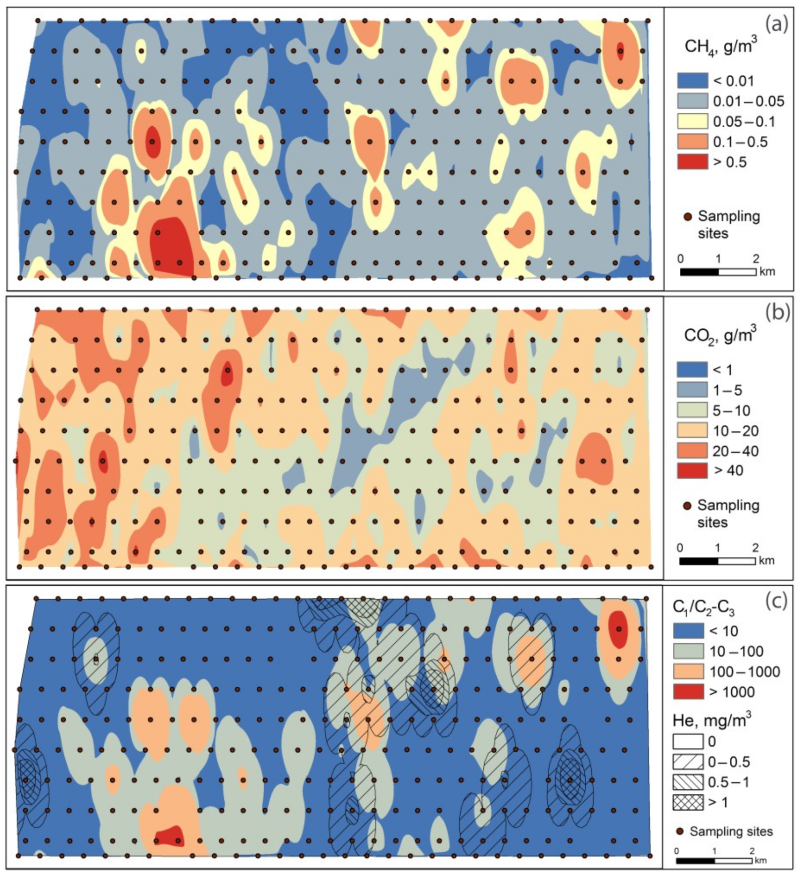
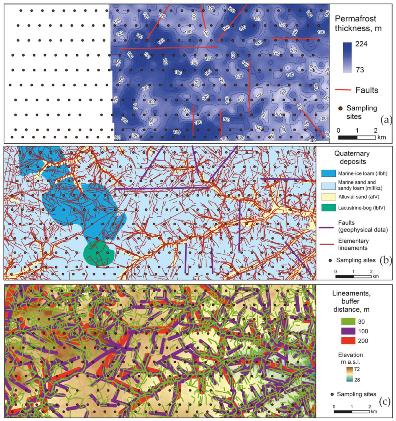


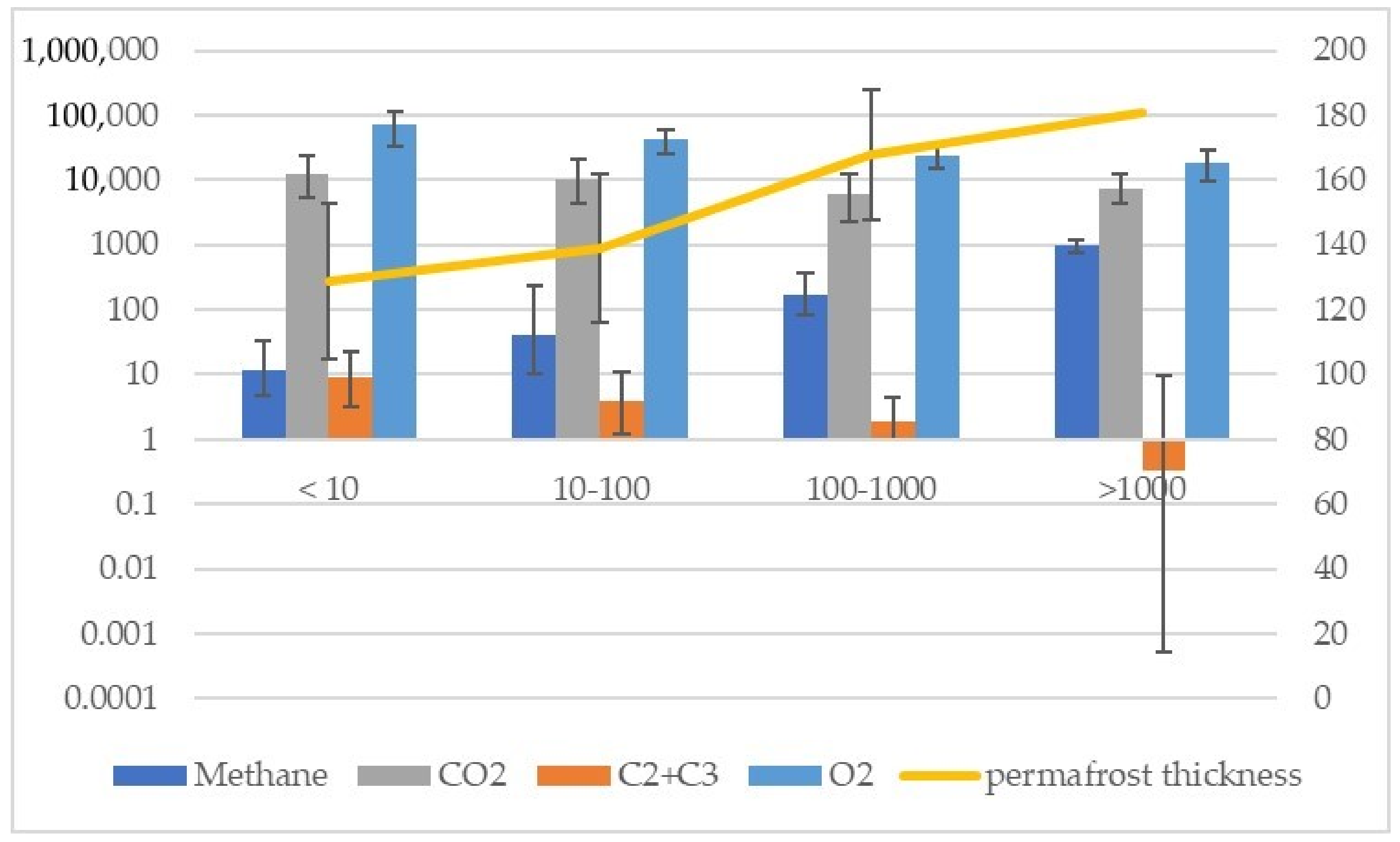
Publisher’s Note: MDPI stays neutral with regard to jurisdictional claims in published maps and institutional affiliations. |
© 2022 by the authors. Licensee MDPI, Basel, Switzerland. This article is an open access article distributed under the terms and conditions of the Creative Commons Attribution (CC BY) license (https://creativecommons.org/licenses/by/4.0/).