1. Introduction
Winter wheat is one of the most widely cultivated and fertilized food crops, and it is used in many products for human consumption [
1]. Wheat growth monitoring is a crucial part of achieving a reasonable yield, and field management is the following step after analyzing the crop growth situation. Among different kinds of field management, fertilizing has been recognized as the most important. Proper fertilizing is the key strategy to secure optimal crop yield. Nitrogen-based fertilizers provide vast N for crop growth. Nitrogen (N) takes part in multiple metabolisms and structural components, which makes N one of the most important elements in both crop and environmental sciences. It is an essential element in both wheat crop growth and yield formation [
2]. While N deficiency makes it difficult to achieve the target yield, overfertilization is a common mistake in the unilateral pursuit of high yield. Excessive N applications lead to delayed maturity, which causes reduced yield, and adverse environmental impacts, such as soil contamination; furthermore, nitrogen is a major contributing source of greenhouse gas (GHG) [
3,
4]. Diagnosing crop growth status and variable rate fertilization can assist in avoiding the above problems. The principle of precision agriculture is the spatial and temporal variability of fertilizer. Therefore, the determination of crop status is the key procedure in practice [
5]. Several parameters have been used for measuring the plant growth condition; for example, plant nitrogen concentration (PNC) and accumulation (PNA) are direct indicators of crop growth. Additionally, above-ground biomass (AGB) is another frequently used indicator because it is the proxy of the final yield. When the parameters are put together, the nitrogen nutrition index (NNI) is established by critical N dilution theory [
6,
7]. These parameters have been proved to be effective for use in variable rate fertilization; however, the issue is the speed of the process [
8].
The timely and accurate monitoring of crop growth status is necessary for modern agricultural management. Traditionally, to acquire the growth variables, field samples are taken for lab analysis, which is time-consuming. Additionally, the results are spatially limiting. Thus, it is important to find a way to achieve more effective results [
9]. Remote-sensing technology offers an alternative for assessing crop nutrient status, and crop parameters have been retrieved from remote-sensed data by different approaches [
10]. With the emerging unmanned aerial vehicle (UAV) platform, which carries passive or active sensors, it is becoming easier to access rapid and non-destructive spatial results of crop growth parameters [
11]. UAVs have advantages of flexibility and versatility; they are operated at relatively low cost while acquiring high spatial and temporal resolution data. In practice, the crop AGB can be estimated by RGB or multispectral images, and other N-related crop parameters can also be estimated by fusing image and spectral information. The reported modeling process includes seeking sensitive bands or VIs, and then using them to build models. Meanwhile, some studies investigated the optimal time window for growth monitoring [
12,
13,
14,
15]. These previous experiments have demonstrated the feasibility of UAV application.
Crop growth variables and retrieval methods can be categorized in three ways: empirical, physical, and hybrid methods. Previous research focused on the simple linear or non-linear relationships between vegetation indices (VI) and specific crop parameters [
12,
16], or used physical-based methods, known as radiative transfer models, to retrieve crop N status [
17]. In order to make full use of the abundant UAV data, including band reflectance, VI or texture, and other features, machine learning regression algorithms of various kinds have been introduced for quantitative vegetation remote sensing [
18,
19,
20]. Machine learning methods are becoming powerful modelling tools to interpret information from large amounts of remotely sensed data. Among different regression algorithms, random forest (RF) is a classic and powerful method [
21]. It is an ensemble learning model that combines a large number of decision trees, which makes it robust when the model consists of many input variables. RF models have been widely used in crop classification, growth monitoring, and yield forecast [
22,
23]. Additionally, RF prevails in the previous comparison studies of different algorithms for monitoring different crops [
24,
25]. These studies have yielded satisfactory results by using RF models, both in classification and prediction, which strongly illustrated the feasibility of the RF model.
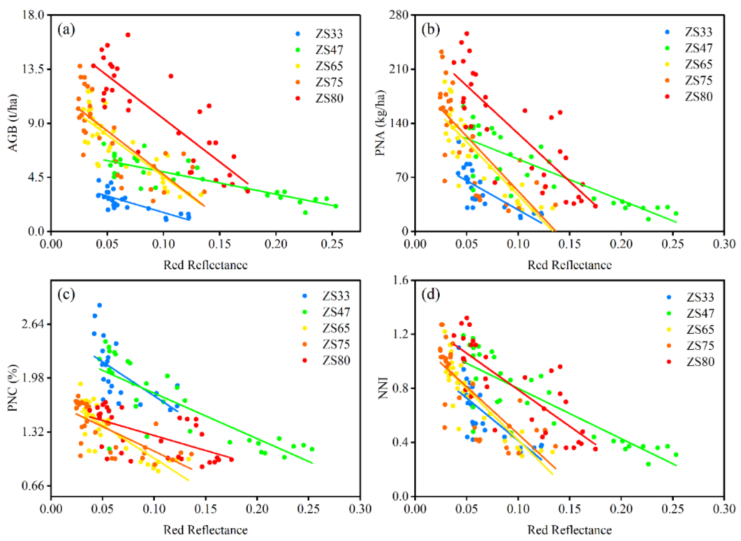
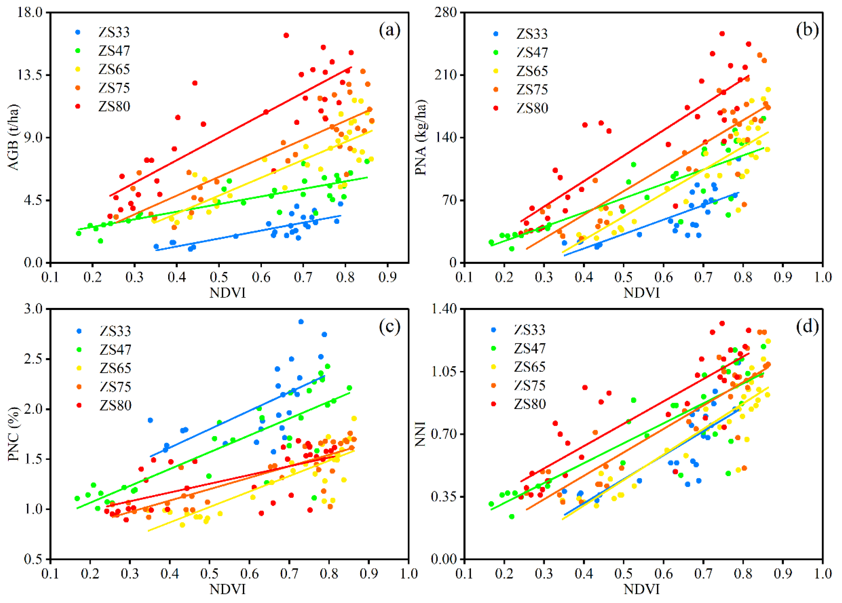
Although crop parameters are estimated by different techniques using remotely sensed data, a common problem is that these kinds of models neglect the fact that crops are significantly different in their different growth stages. Crop growth is an allometry process. The morphology traits of a crop can change substantially from the vegetation to reproductive stages, and the leaves, stems, and spikes play different roles in different stages. This would cause significant impacts on remote-sensing observations. In the practice of crop vegetation remote sensing using optical sensors, the leaves, stems, and panicles are the spectrally responsive organs. Leaves are always the major sources of reflection in the different stages [
26]; however, as the growth stages progress, leaves will transform from a sink to a source of assimilates. When leaves are sinks, their major function is as the storage warehouse of photosynthesis production, while they turn into a photosynthesis producer when the leaves are mature. At the same time, the stems start to become the major storage of the assimilates, especially after the shift from the vegetation to the reproductive stage, and the panicles become the new sink for the yield formation. During this period, the characters of the leaves, stems, and panicles keep changing, affecting sink and flow interrelation and transformation; consequently, biomass and N deposits will translocate in different sinks accordingly [
27], id est, the leaves will provide substantial reflectance while not always being responsible for the majority of crop biomass and nitrogen storage. Since this asymmetric information is hard to be exhibited in spectral information [
28], it might explain the deficits of the simple linear model; furthermore, this phenomenon suggests that phenology information should be considered in the crop monitoring models. Several researchers have pointed out that crop phenology is important in predicting crop growth conditions or forecasting yield [
29,
30].
Current machine learning models for monitoring crop growth status have been established by solely using multiple vegetation indices [
12,
31]. In addition to this, efforts include fusing color features or combining them with cultivar information [
32,
33]. Moreover, canopy fluorescence is an increasingly popular technique that can be used for growth monitoring [
34]. Furthermore, using spectral-based deep learning is also a rational approach [
35]. These studies utilized spectrum information in addition to other vegetation characteristics. Only a few studies considered the variation of phenology and integrated it into the model. Since the crop growth status significantly varied from stage to stage, optical sensors had a limited ability to track this inherent variation. The addition of different types of data could be descriptive for different stages, which clearly showed that the direct application of phenology is appealing in the context of adjusting the model instability in multi-stage scenarios. Therefore, the main objectives of this study are:
- (1)
To verify the phenology effect on retrieving wheat crop parameters from UAV multispectral data;
- (2)
To use RF models to evaluate the accuracy of different combinations of band reflections, Vis, and PIs in wheat parameters prediction;
- (3)
To Specify the accuracy of different growth stages and N treatments in established models to understand the model applicability.
2. Materials and Methods
2.1. Experimental Site and Design
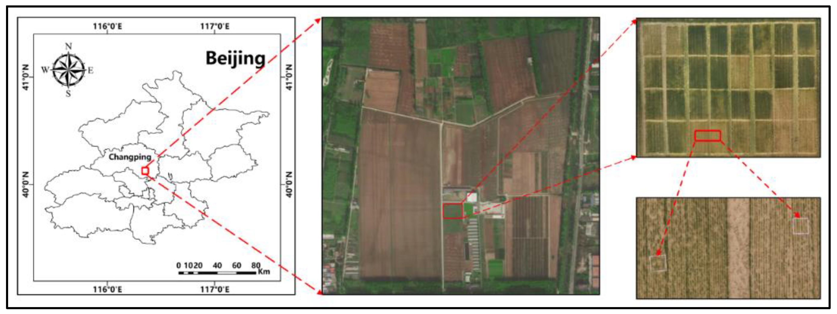
We conducted the experiment during the 2020–2021 winter wheat growing season at the Xiaotangshan National Experiment Station for Precision Agriculture (116°26’36’’ E, 40°10’44’’ N) in Beijing, China (
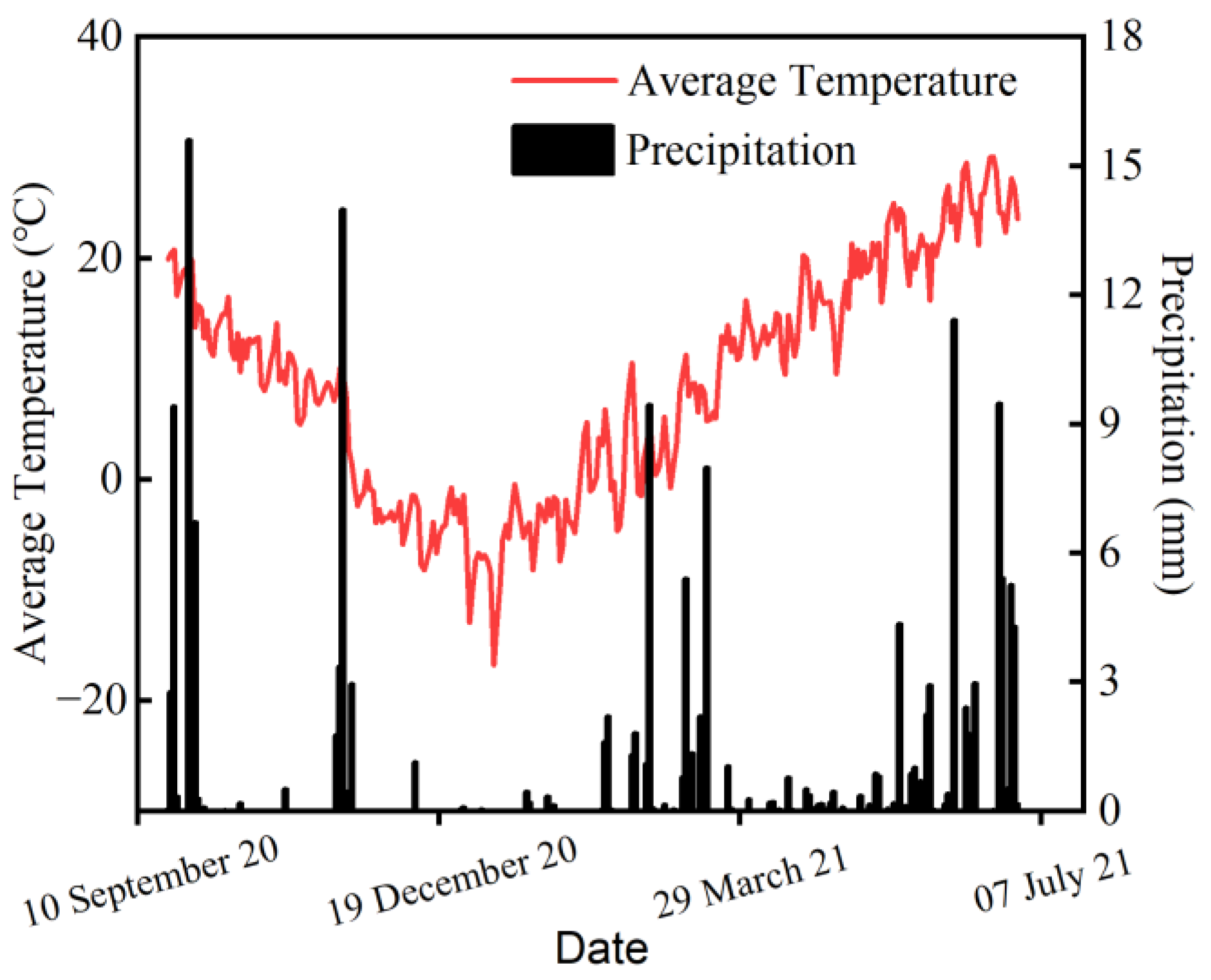
Figure 1). The field site is in the northernmost section of the North China Plain, which has a temperate monsoon semi-humid climate of medium latitudes, with an average altitude of 36 m. It has an average annual precipitation of 500–600 mm and an average annual temperature of 12 °C. The annual amount of solar radiation is 4800 MJ m
−2 (China Meteorological Data Service,
http://data.cma.cn/ accessed on 6 January 2022). We provide the weather information of the experiment duration in
Figure 2.
This study was part of an ongoing long-term fertilizer experiment. We selected two local wheats (Triticum durum L. cultivar. JH11 and cultivar. ZM1062) and four nitrogen fertilizer rates (0, 90, 180, 270 N/ha) in the field experiment. The plot size was 9 × 15 m. We set row spacing to 15 cm, and we uniformly set the plant density to 360 × 104 plants ha−1. We settled treatments in all field experiments using a complete randomized block design with four replicates. We divided the nitrogen fertilizer application into two splits and applied 1:1 for the base and top-dress before sowing and at the jointing stage.
The primary soil type is a clay loam soil by Food and Agriculture Organization (FAO) soil classification, with a pH of 7.7, 19 gkg−1 organic matter, 1.01 gkg−1 total N, 14.5 mgkg−1 Olsen-P, and 127.9 mgkg−1-available K in the 0–20 cm-surface soil layer. We performed other field management procedures, including weed control, pest management, and our application of phosphate and potassium fertilizer followed local standard practices for winter wheat production.
2.2. Crop Data Acquisition and Calculation of Nitrogen Nutrient Index
We conducted five experiments in five key wheat growth stages (jointing, booting, anthesis, early filling, late filling). There were 24 samples in the jointing stage and 32 in the other stages. In total, the sampling number was 152. During field sampling at each stage, we randomly collected 20 tillers around the white frame of each plot. We immediately took fresh samples to the laboratory and separated them into leaves and stems, and also spikes after they emerged. We put the samples into paper bags and placed them in the oven at 105 °C for 20 min to stop metabolism, and then dried at 80 °C until the samples became constant weight. We recorded the dry weight of each sample by a balance with an accuracy of 0.001 g. After we acquired the AGB, we analyzed all samples for N concentration using the micro-Kjeldahl method. We calculated the total plant N concentration as the ratio of the total N accumulation to AGB.
where
LW,
SW, and
PW are the dry weights of leaf, stem, and panicle samples, respectively.
LN,
SN, and
PN are the N concentrations of leaf, stem, and panicle samples, respectively.
T is the number of winter wheat stems per unit area and L is the row spacing (15 cm). Subsequently, PNA is plant nitrogen accumulation and PNC is plant nitrogen content.
As described by Lemaire [
36], we calculated the nitrogen nutrition index (NNI) of each treatment within various growth stages by the following equation:
where the
Na represents the actual N concentration,
Nc represents the critical N concentration. The
Nc curve used in this study was adopted from previous research [
37]:
We established the equation from a previous nitrogen fertilizer experiment in the same field. Crop nitrogen status is normal when NNI is between 0.95 and 1.05, it overdoses when NNI exceeds 1.05, and there is a deficit when it is less than 0.95.
2.3. Acquisition and Preprocessing of UAV Images
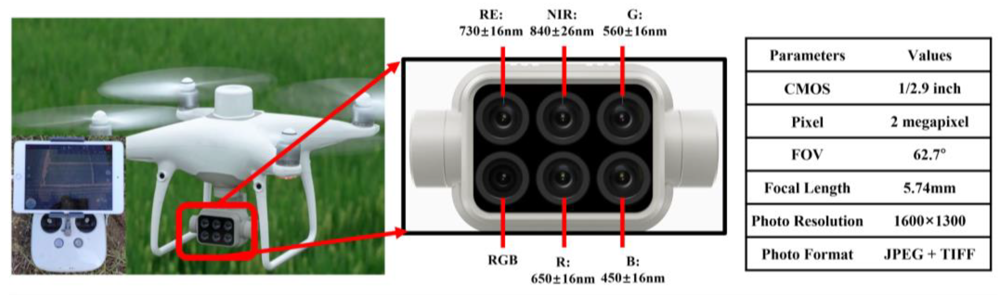
We used a DJI Phantom 4 Multispectral 4-rotor-wing unmanned aerial vehicle (UAV) (DJI-P4M, SZ DJI Technology Co., Ltd., Shenzhen, China) to capture multispectral images. The UAV had 2 million pixel multispectral sensors consisting of 6 cameras, including Blue (450 nm ± 16 nm), Green (560 nm ± 16 nm), Red (650 nm ± 16 nm), RE (730 nm ± 16 nm), NIR (840 nm ± 26 nm), and visible light (RGB). The details of the UAV and sensor information are in
Figure 3.
We conducted five flights within each key wheat growth stage. We set the flight mission height to 30 m, with a speed of 4 m/s. We set the image overlap and sidelap to 80%. The ground spatial resolution is 1.6 cm under such parameters. We performed all flight missions between 10:00 and 12:00 on clear and cloudless days. Prior to each flight, we collected calibration images with a standard reflectance panel. The panel is a fine cloth installed inside a plastic box, and it has a basic reflectance of 0.797, 0.872, 0.877, 0.875, and 0.867 for Blue, Green, Red, RE, and NIR, respectively. We calibrated each image to follow the specific band. After the flight, we calibrated our collected multispectral images and processed into ortho-mosaic maps using DJI Terra software (Terra, SZ DJI Technology Co., Ltd., Shenzhen, China) for further analysis.
2.4. Feature Extraction and Determination
We used the ortho-mosaic maps for band reflectance and VIs extraction. We extracted all data within the white frames using shapefiles for each stage. Additionally, we calculated plot average of all pixel values as the extraction results.
We used three types of features in this study, including the original multispectral band reflectance as the first type, vegetation indices for the second type, and phenology indicators (PIs) for the third type. For the first two types of data, because we extracted them from UAV images, in order to keep consistency, we acquired all of them from within the white frame (
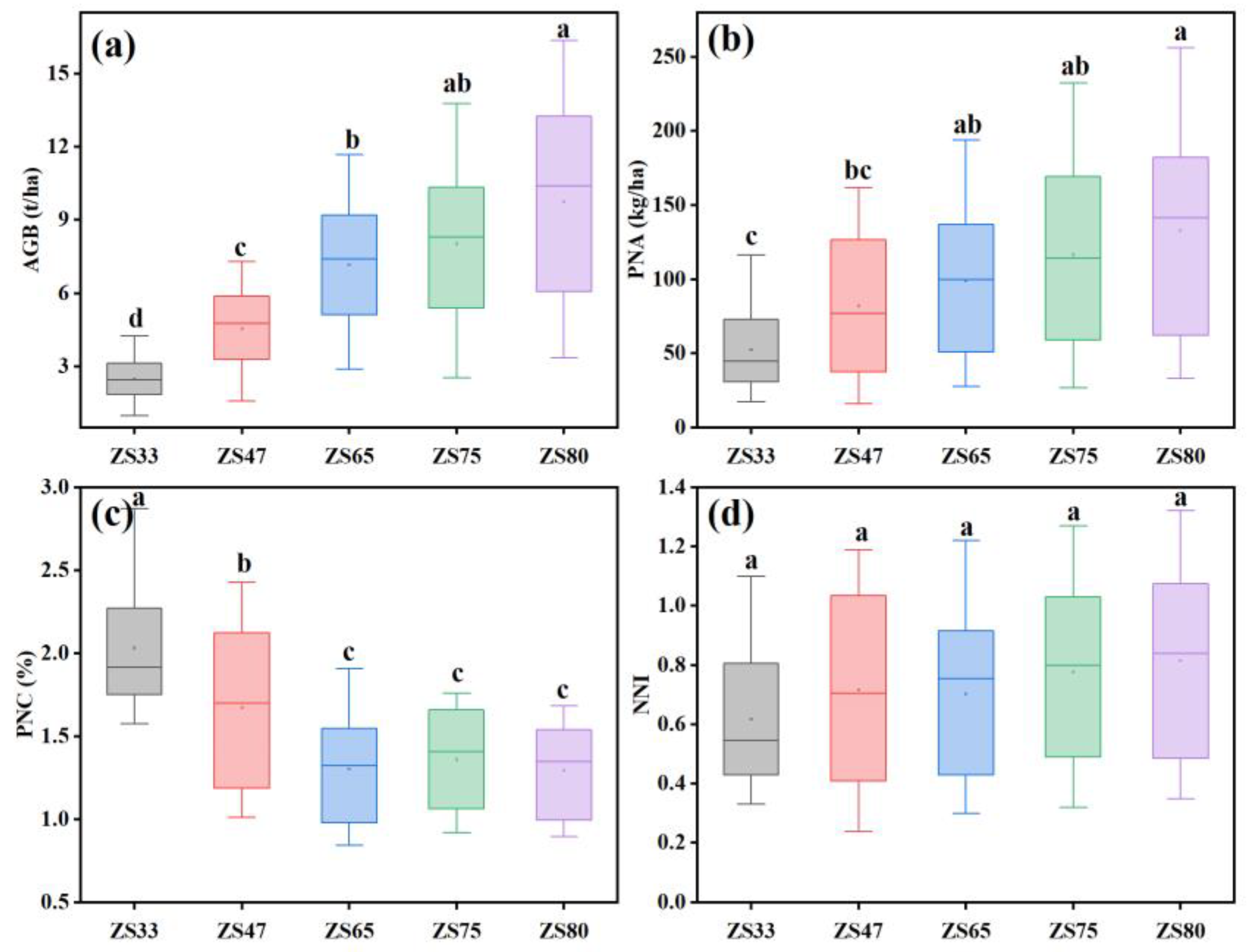
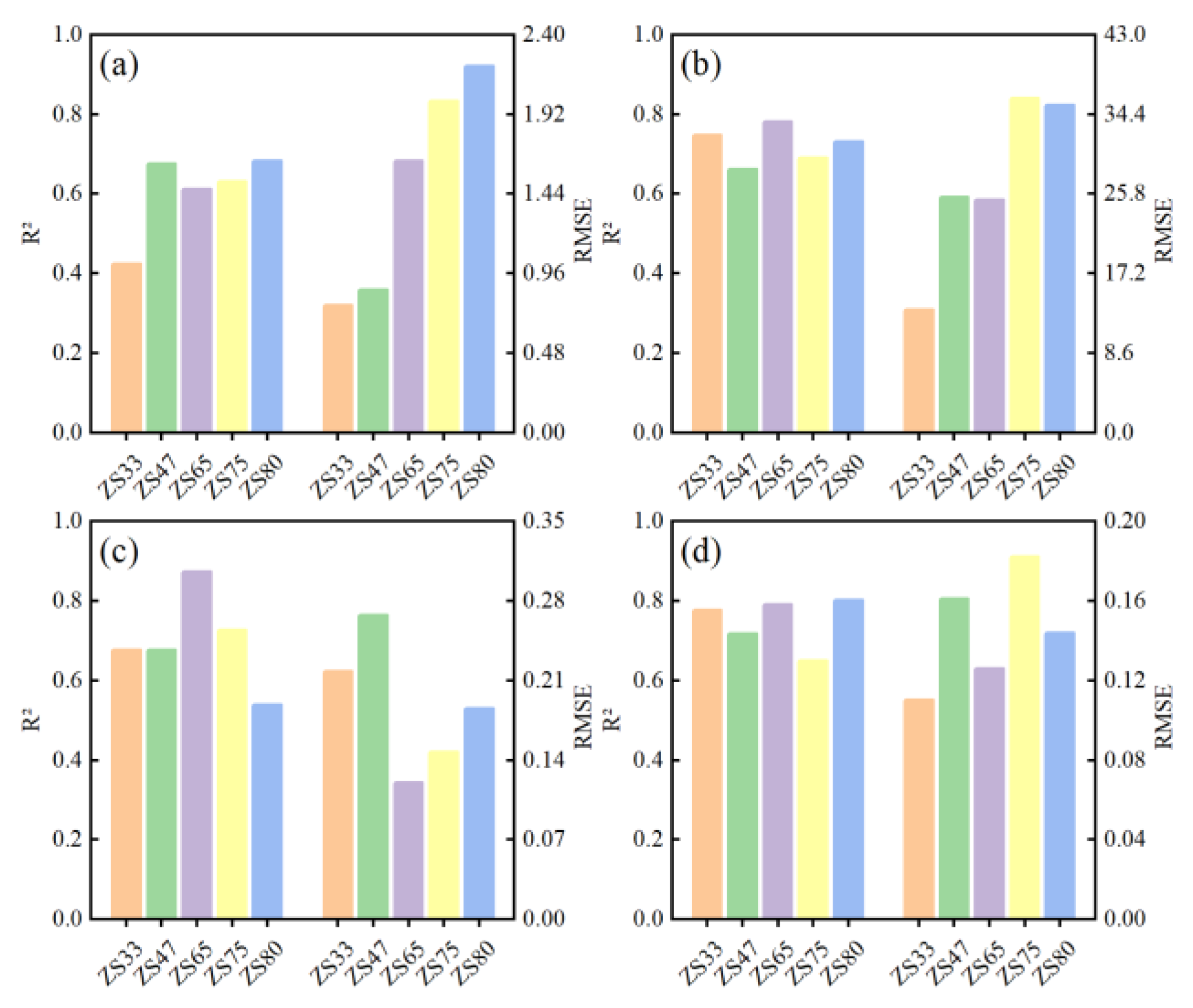
Figure 1). We collected the original reflectance of each band as the first data type, and then we selected several vegetation indices as second data type, of which we used part of them to model AGB. Additionally, we used part of them to retrieve key growth parameters in the previous studies, which indicated all the selected VIs have reasonable potential to be used for crop nitrogen status monitoring. As for the third type, we recorded the five stages that represent the typical wheat growth process as Zadok growth stages—phenology indicators. In this case, ZS33, ZS47, ZS65, ZS75, and ZS80 represent the wheat jointing, flag leaf, anthesis, early filling, and late filling stages, respectively. In order to maintain data uniformity, we simplified the phenology into a number of stages. The three types of data are listed in
Table 1.
2.5. Data Analysis and Model Establishment
We analyzed the 4 crop parameters data by Tukey’s HSD test to distinguish the differences across 5 stages. We performed a three-way analysis of variance (ANOVA) to explore how much the phenology contributes to the biometrics. We analyzed the effects of cultivars, N treatment, and phenology on AGB, PNA, PNC, and NNI. We used Duncan’s test to analyze differences in parameter averages between treatments. The threshold for statistical significance was p < 0.05.
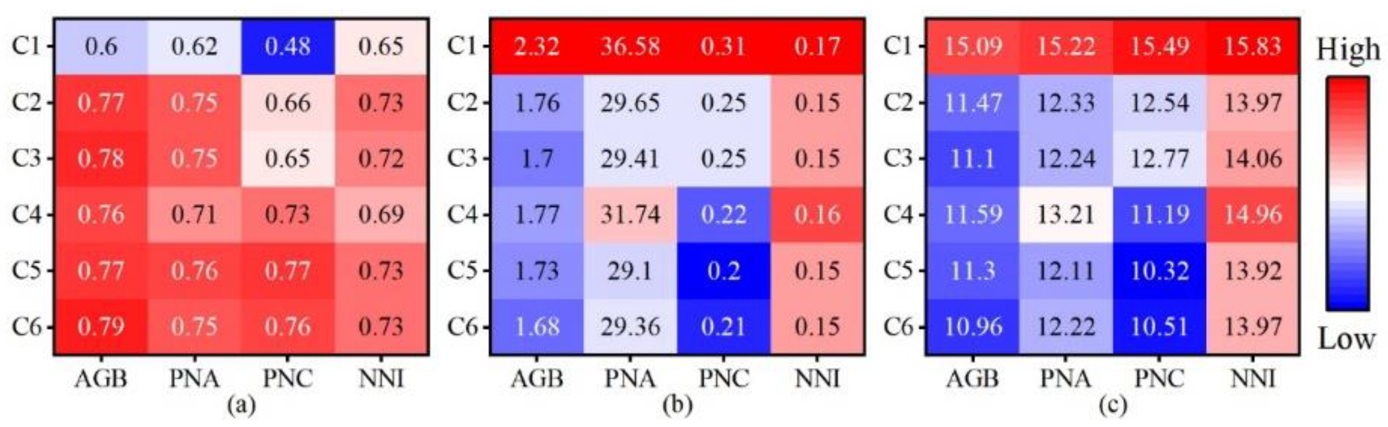
In this study, we employed RF to build models for AGB, PNA, PNC, and NNI. As mentioned above, we grouped all the features into three types of data, and we selected these features as six combinations (
Table 2).
RF is an ensemble technique that combines multiple decision trees, and each tree in the forest predicts independently. We put all predictions into a vote to make the final prediction. It is a practicable model when dealing with small sample sizes. RF models involve a hyperparameter-adjusting process to maximize the accuracy of the models. Thus, we optimized the models’ hyperparameters through 10-fold cross-validation. The only parameter in random forests that typically need optimization are the number of trees in the ensemble. We settled on a total of 200 decision trees for the model based on the stable results from primary validation. We also used the number of decision trees in related remote-sensing studies [
50].
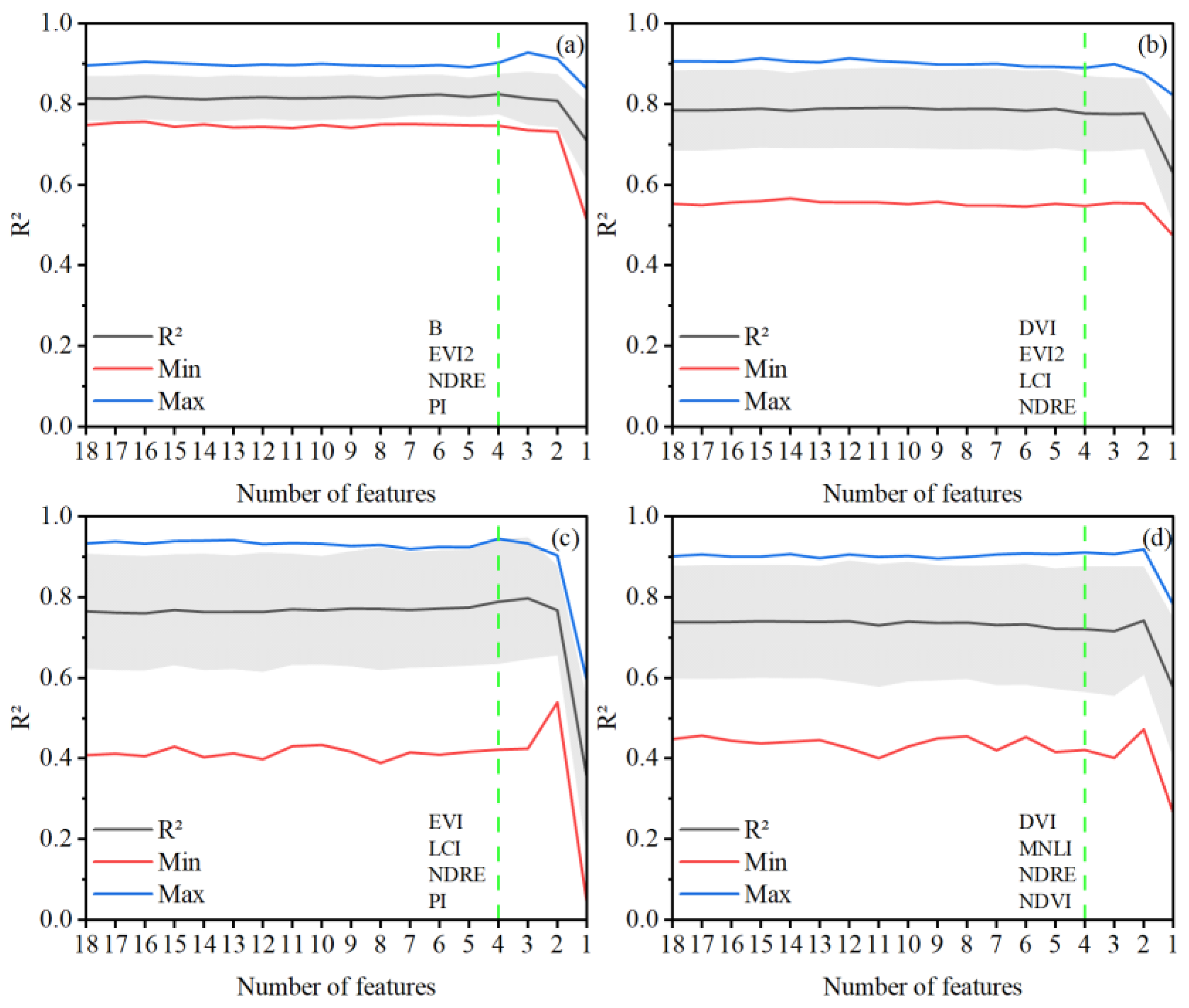
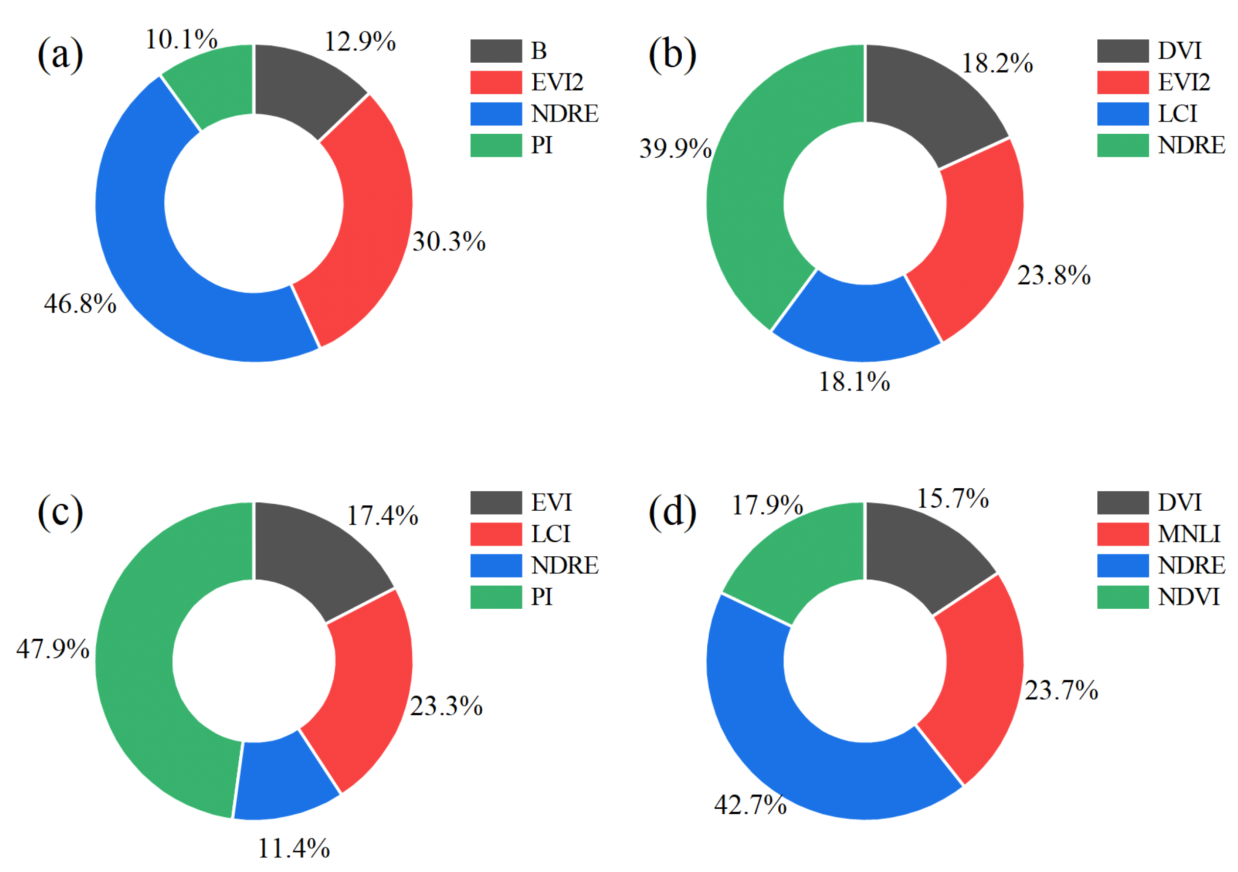
To analyze the special effects of our most interesting PIs we performed multiple iterations to deconstruct the model feature by feature. Firstly, we ranked each feature based on the Bayesian framework; therefore, the ranking result can be used as a feature reduction tool. Then, we removed the lowest relevant feature in each iteration. Eventually, we found the most sensitive features. Through iterations, we determined the minimum number of features to build a model while keeping the accuracy acceptable.
2.6. Model Evaluation
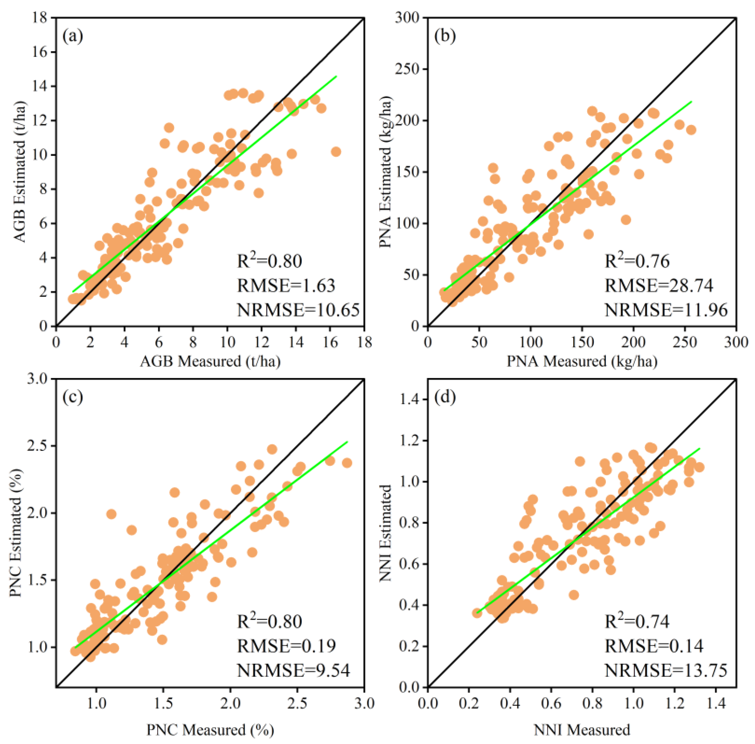
We built and evaluated all models by 10-fold cross-validation, and we used the mean results of cross-validation in the model comparisons. We used three commonly used indices (R
2, RMSE, and NRMSE) to compare the performance of generated models The calculation equations of R
2, RMSE, and NRMSE are as follows:
where
and
are the measured and predicted values for sample
, respectively.
indicates the mean values and
is the number of samples used for calibration or validation set.
is the average value of the samples.


 ,
, 


