Abstract
Polarimetric synthetic aperture radar (PolSAR) image classification is a pixel-wise issue, which has become increasingly prevalent in recent years. As a variant of the Convolutional Neural Network (CNN), the Fully Convolutional Network (FCN), which is designed for pixel-to-pixel tasks, has obtained enormous success in semantic segmentation. Therefore, effectively using the FCN model combined with polarimetric characteristics for PolSAR image classification is quite promising. This paper proposes a novel FCN model by adopting complex-valued domain stacked-dilated convolution (CV-SDFCN). Firstly, a stacked-dilated convolution layer with different dilation rates is constructed to capture multi-scale features of PolSAR image; meanwhile, the sharing weight is employed to reduce the calculation burden. Unfortunately, the labeled training samples of PolSAR image are usually limited. Then, the encoder–decoder structure of the original FCN is reconstructed with a U-net model. Finally, in view of the significance of the phase information for PolSAR images, the proposed model is trained in the complex-valued domain rather than the real-valued domain. The experiment results show that the classification performance of the proposed method is better than several state-of-the-art PolSAR image classification methods.
1. Introduction
Synthetic Aperture Radar (SAR) has been a highly sought-after and powerful remote sensing technology due to its all-weather, all-time, and high-resolution imaging capabilities, and it has been widely used in many fields. Early SAR was single-polarized (also called single-channel), which made it difficult to completely express the target-scattering characteristics. Compared with the single-polarized SAR, polarimetric synthetic aperture radar (PolSAR) is a multi-channel SAR system with more discriminative information. PolSAR can clearly describe the polarized scattering characteristics of complex ground targets by sending and receiving electromagnetic waves in different combinations. Thanks to the more abundant polarimetric target-decomposition features and complex-valued information, PolSAR data interpretation has attracted many researchers’attention, and a large number of approaches have been proposed in recent years. Polarimetric target decomposition is one of the most influential approaches for PolSAR image classification. The essence of polarimetric target decomposition is polarimetric measurement data, such as scattering matrix, covariance matrix, coherent matrix, and so on, which are decomposed into various components. Researchers have studied polarimetric target decomposition for a long time, and numerous approaches have been put forward, such as Krogager decomposition [1], Cloude–Pottier [2], Freeman decomposition [3], Pauli decomposition [4], Huynen decomposition [5], and so on. Furthermore, some machine learning algorithms have broken the limitations of traditional algorithms and have made great achievements in the field of PolSAR image classification, such as the Wishart Classifier [6], Bagging [7], the Support Vector Machine (SVM) [8,9], and Random Forest (RF) [10,11].
In recent years, deep learning (DL) technology has shown significant superiority over traditional machine learning approaches. Prominent success using DL technology has been made in various fields, such as speech recognition [12,13], natural language processing [14], computer vision [15,16], semantic segmentation [17,18], and outlier detection [19]. This is mainly attributed to the deep multi-layer structure of DL that enables the network to have the ability to learn discriminate, invariant, and high-dimensional features of data automatically, as well as to their end-to-end training schemes [20]. DL has a strong capability to learn a series of abstract hierarchical features from raw input data and obtain a task-specific output. Therefore, DL technology provides an entirely new method for PolSAR image classification, and many classification methods have been proposed, such as Wishart deep belief network (WDBN) [21], Wishart-auto-encode (WAE) [22,23,24], sparse autoencoder [25,26], the long short-term memory (LSTM) network [27], semisupervised deep learning model [28,29], deep reinforcement learning [30], and convolutional neural network (CNN) [31,32,33]. CNN has made impressive achievements in the field of PolSAR image classification among these DL methods, and it consists of several successive convolution layers, pooling layers, and fully-connected layers. It is well-known that SAR has limited labeled data, and using CNN architectures in the SAR domain with limited data benefits from transfer learning [34,35,36]. Huang et al. [37] proposed a deep transfer learning method to solve the problem of highly imbalanced classes, geographic diversity, and label noise of SAR data. Two transfer learning strategies are proposed in reference [38], which adopt the FCN and U-net architecture for PolSAR image segmentation with small training sets.
As we all know, the essence of PolSAR image classification is that each pixel is classified into different terrain classes with the corresponding physical characteristics, but the input of the CNN classification framework is an image and the output is a single categorization vector. This approach has several disadvantages. First, it is very expensive in terms of storage. For example, if each pixel uses an image block with a size of 5 × 5, the required storage space increases sharply with the number and size of sliding windows. Second, the computational efficiency is low. Since adjacent pixel blocks are basically repeated, calculating the convolution for each pixel block one by one is also repetitive to a large extent. Finally, pixel block size limits the receptive field. Usually, the size of the pixel block is much smaller than the size of the whole image, so only some local features can be extracted.
The fully convolutional network (FCN) proposed by Long et al. [17] was considered the landmark network in semantic segmentation, since it first constructed an end-to-end, pixel-to-pixel scheme and obtained tremendous results. The framework of FCN discards the last fully connected layers of the traditional CNN replaced by three convolutional layers, aiming to maintain the 2-D characteristics of raw input rather than the one-dimensional vector of class scores and to address pixel-wise issues. In addition, the FCN can input arbitrary-sized images and output a label map the same size as the input [17]. Therefore, the FCN is more tailored to PolSAR image classification against CNN, which is confirmed by plenty of methods. Li et al. [39] proposed a sliding-window FCN (SFCN) and sparse coding (SFCN-SC) to classify PolSAR images. Chen et al. [40] further introduced adversarial reconstruction-classification networks (RCN) and adversarial training based on SFCN. Fariba et al. [41] proposed a new Fully Convolutional Network (FCN) architecture that is specifically designed for the classification of wetland complexes using PolSAR imagery. Based on the manifold hypothesis, He et al. [42] proposed a PolSAR image classification method by combining nonlinear manifold learning with a full convolution network. Mullissa et al. [43] presented a PolSARNet that uses real-valued weight kernels to perform the pixel-wise classification of complex-valued images. Cao et al. [44] first proposed complex-value FCN (CVFCN), which extended real-value FCN to the complex-valued domain. What is more, Adugna et al. [45] proposed the multistream complex-valued FCN.
Although FCN has achieved prominent breakthroughs for PolSAR image classification, there are still several flaws. Firstly, we find that the phase information of PolSAR images is rarely taken into count in the existing FCN architectures. However, the phase of off-diagonal elements of the covariance or coherency matrix is crucial in identifying different types of scatterers [46]. Secondly, each encoder and decoder operation of existing methods perceives and outputs a single receptive field for one pixel, which may limit the receptive fields. Thirdly, the limited labeled samples are still a challenge for PolSAR image classification.
In view of the above challenges, this paper presents a multi-scale, fully convolutional network with stacked dilated convolutions for PolSAR image classification in the complex-valued domain, which is named CV-SDFCN for short. We firstly enlarge the labeled samples of PolSAR image by combining the semi-supervised fuzzy c-means (SSFCM) algorithm with Wishart distribution, which is described our previous work [47]. Then, this paper constructs the Complex-valued Stacked Dilated Convolutions (CSDC) with different dilation rates to take full advantage of the phase information of PolSAR data as well as to produce a multi-scale response and dense outputs. Finally, we reconstruct the encoder–decoder structure combined with CSDC layers, which is appropriate for a small number of training samples. The major contributions of this paper can be summarized as follows:
- (1)
- Considering the importance of phase information of PolSAR image and the influence of receptive fields size, the standard convolutions in the FCN model are replaced by stacked-dilated convolutions with different dilation rates in a complex-valued domain. This allows each pixel to have several receptive fields and to capture multi-scale features.
- (2)
- To avoid the calculation burden caused by stacked multiple dilated convolutions, the sharing-weights strategy is adopted in each CSDC layer.
- (3)
- Considering the problem of lacking labeled samples of PolSAR images, the encoder–decoder structure of the FCN model has been reconstructed with our method.
The remainder of this article is arranged as follows. Section 2 shows the polarimetric representation of PolSAR images. Section 3 introduces some related works. Section 4 formulates the proposed methods in detail. In Section 5, experimental results for three PolSAR images are exhibited, and a detailed discussion is given. Finally, Section 6 gives the conclusion and describes our future work.
2. Representation of PolSAR Images
By transmitting and receiving antennas in different polarization states, PolSAR data are able to capture four types of polarization channel information: , , , and . The complex scattering matrix [48] is used to describe the electromagnetic scattering characteristic of the ground objects. The complex scattering matrix is given by:
Reciprocity decides that the two cross-polarized echoes should be identical in the case of monostatic backscattering, i.e., . The complex scattering vector k of the matrix in the Pauli decomposition can be calculated as [23]:
In general, the scattering characteristics of terrain targets can also be described by polarimetric coherency or covariance matrices [49]. The polarimetric covariance matrix is represented as
where the superscript H denotes conjugation transpose operation, and is the ith scattering vector. The polarimetric coherency matrix T is a Hermitian positive semidefinite matrix: the main diagonal elements are the real number, while the off-diagonal element is a complex number. In addition, the off-diagonal elements are conjugate-symmetric about the main diagonal.
3. Related Work
We introduce the basic principle of dilated convolution and the structure of FCN model in this section.
3.1. Dilated Convolution
Dilated convolution is a particular convolution operator in which the receptive field size varies with the number of intervals between kernel weights, which was first proposed by Yu et al. [50]. The intervals between convolution kernel are also named dilated factors. The dilated convolution provides a method to exponentially increase the receptive fields of the network by linearly enlarging the size of convolution kernels without losing resolution. Accordingly, dilated convolutions work well in generating dense feature maps among deep neural networks, which is quite promising for pixel-level tasks.
For a 1-D case, if we represent the input data as and the convolutional kernel as w, separately, the dilated convolution is illustrated as:
where represents the output and r denotes a dilated factor that determines the intervals between the kernel weights. If the dilated factor is 1, the dilated convolution is equal to the standard convolution.
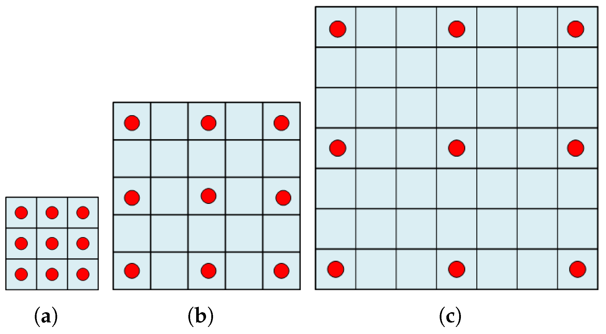
For a given 2-D case, dilated convolutions with are presented in Figure 1, separately. As shown in Figure 1, the main idea of dilated convolution is that () zeros are inserted in between adjacent pixels of standard convolutions. For example, if given a standard kernel with the size of and , the receptive field of dilated convolution will be . As is shown in Figure 1, the size of the receptive field changes with the dilated factor; meanwhile, there are no any additional parameters.

Figure 1.
The dilated convolution with a different dilated factor. (a) denotes the dilated convolution with . (b) denotes the dilated convolution with . (c) denotes the dilated convolution with .
3.2. Fully Convolution Network
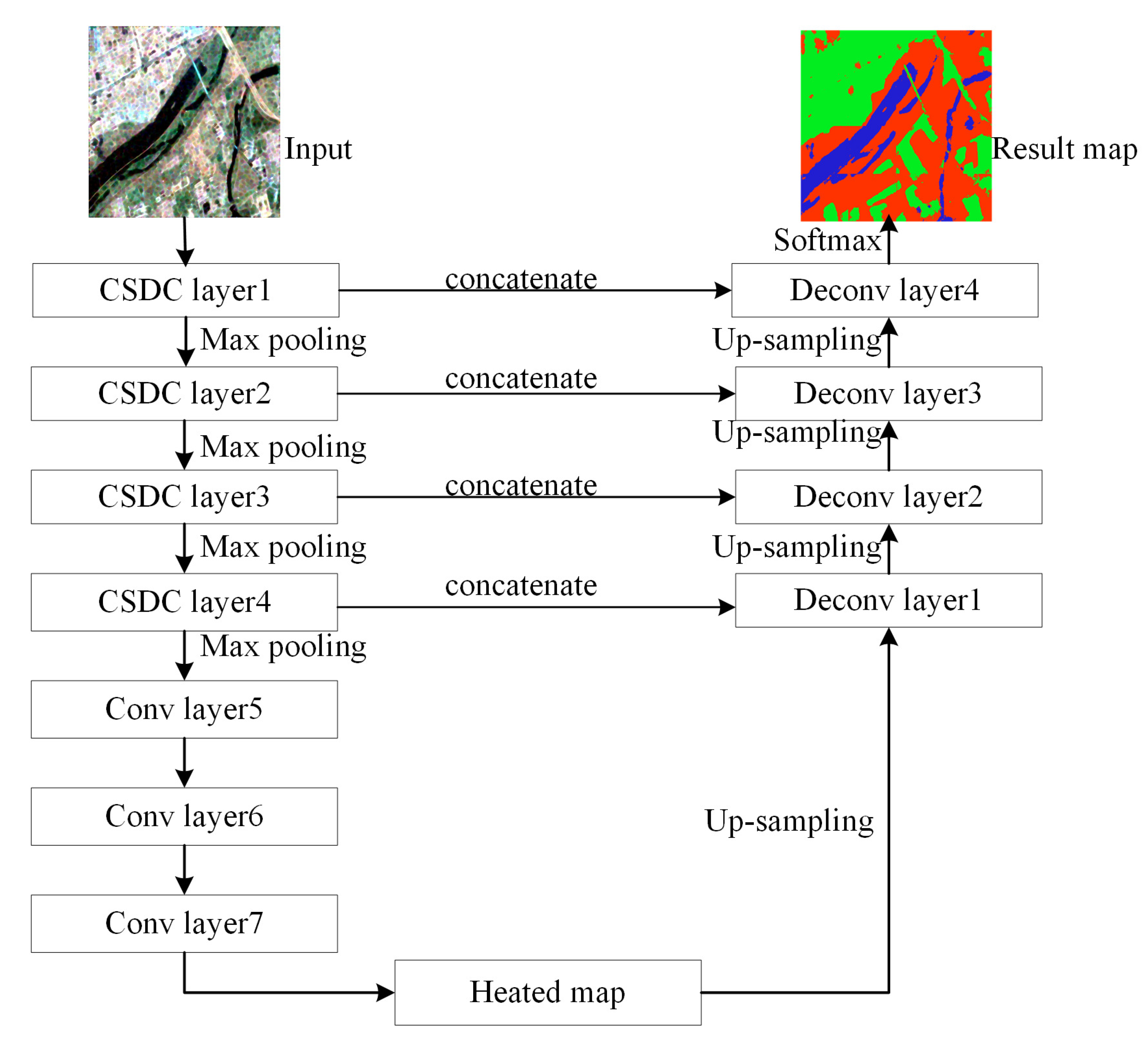
FCN was originally designed for image semantics segmentation, which can achieve end-to-end, pixel-to-pixel training [17]. Unlike the classic CNN model, FCN is the first encoder–decoder network to directly segment image semantics at the pixel level [51]. The pioneering idea of the FCN model is that the last fully connected layers of CNN are substituted by convolutional layers with the kernel size , where the output features are high-dimensional “heated maps” rather than a single categorization vector. Removing full connection layers allows the input images to be arbitrary in size, because of “heated maps” via several convolutional layers, Relu layers, down-sampling layers, and others. In the decoder stage, up-sampling is required to restore the “heated maps” to the same size as the input because down-sampling results in the reduction in spatial dimensions [52]. To refine the spacial precision of the output and combine layers of the feature hierarchy, a skip connection is employed to fuse coarse layers and fine layers that effectively combine “where” with “what” [17]. Finally, a category matrix is generated as the same size as the input and the category probability of each pixel is scored via a softmax classifier. The framework of FCN is shown in Figure 2.

Figure 2.
The framework of FCN.
4. Methodology
This section describes the concrete implementation of the proposed method. First, we extend the dilated convolutions to the complex-valued domain and construct a complex-valued stacked-dilated convolution to maintain a high solution feature map and capture multi-scale PolSAR information. Moreover, we introduce a new encode–decode FCN model combined with CSDC. To alleviate the calculation burden and speed up the convergence of the proposed model, we employ the strategy of shared weights. Finally, some labeled pixels are randomly selected for model training. The total labeled samples in the ground truth are utilized to certified the classification effectiveness, and the final visual classification results are obtained by our proposed method.
4.1. Complex-Valued Dilated Convolution
Both amplitude and phase information are crucial for the feature representation of PolSAR images. Therefore, we expand real-valued dilated convolution to a complex-valued domain. For complex-valued dilated convolution, the input is represented as (), where and are the real part and the imaginary part of an image, respectively. In addition, the convolutional kernel is represented as , where r and i are also the real part and imaginary part, respectively. We record the dilated convolution operation in Equation (4) as , and the output of the complex-valued dilated convolution can be defined as [53]:
The complex convolution operation can be considered a cross operation. We also extend the general Relu function to the complex-valued domain, which can be represented as [51]
4.2. Complex-Valued Stacked Dilated Convolution
The receptive field is significant for pixel-level assignment. Small convolutional kernels can only extract local characteristics and ignore global context information. For most neural networks, the sub-sampling layers or pooling operator are adopted to increase the receptive field at the cost of resolution, which results in losing some spatial hierarchical information and breaking the internal structure of the original image [47].
As described in Section 3, dilated convolution can enlarge the receptive field with additional parameters, so it is an appropriate solution for pixel-wise classification. Replacing the max-pooling operation or stride-convolution layer with the dilated convolution can not only maintain the high resolution of feature maps in FCN but also maintain the receptive field of the corresponding layer [54]. However, there exists a theoretical issue on dilated convolutions, which is called the “gridding effect” [55,56]. If the standard convolution kernel is and the dilated kernel is , where , the information of pixel in the dilated convolutional layer l comes from that in layer computers with dilated convolution kernel . As described in Section 2, dilated convolution refers to inserting “zeros” into the standard convolution kernel, so the size of output will be when computes with a size of the convolution kernel. For example, if , and the , and only 9 of the 25 pixels in the receptive field participate in the computation. Pixels can only view the information in a “gridding” fashion that would result in a loss of information in a small area and irrelevant information in a large area. Therefore, using dilated convolution directly in the FCN model would make the input too sparse, which may be bad for the feature extraction of PolSAR images.
In order to increase the receptive field and avoid the “gridding effect”, Wang et al. [57] proposed a U-net variant by employing a standard convolution followed by multiple dilated convolutions for the segmentation of medical images. Considering the phase information of the PolSAR image, we construct a noval stacked dilated convolution in a complex-valued domain with different dilation rates to produce a multi-scale response and dense outputs for PolSAR image classification. Unlike Wang et al., we stack three succeeding layers as a block and change their dilated rate as , respectively. In other words, a dilated black consists of three dilated convolutional layers with different dilated rates.
The framework of the CSDC layer is shown in Figure 3. As shown in Figure 3, each CSDC layer consists of three dilated convolutions, and the parameters of a CSDC layer are more than a standard convolution. Replacing all of the standard convolutions in the FCN model with CSDC would directly increase the memory consumption and the calculation burden. Based on the above considerations, we provide a new strategy within the CSDC layer: shared weight. A CSDC layer uses the same kernel and only alters the dilated rate of each sublayer for different scales. As mentioned previously, dilated convolution just inserts “zeros” in standard convolutions; therefore, it is reasonable to share weights in stacked convolutions within a CSDC layer. By sharing weights, the parameters of CSDC layer could be reduced by two-thirds.
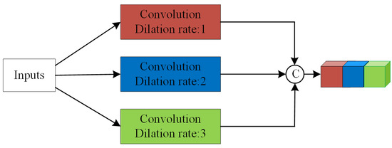
Figure 3.
The framework of the CSDC layer.
4.3. Complex-Valued Stacked Dilated Fully Convolutional Network
It is well known that the labeled samples of PolSAR images are not enough. As a variant of the FCN model, U-net is usually a good choice for small training sets for semantic segmentation [58]. It has an encoder–decoder architecture with several shortcut connections between the two modules to incorporate multilevel features.
In this paper, to achieve good results for PolSAR image classification with a small training set, we construct an encoder–decoder architecture of the FCN model in a complex-valued domain named the CV-SDFCN model, which is based on the U-net model. The overall framework of the proposed method is exhibited in Figure 4. In the encoder, the standard convolution layer of FCN framework is replaced with the CSDC layer.

Figure 4.
The overall framework of the proposed method.
The proposed CV-SDFCN consists of four CSDC layers and three standard convolutional layers. Each CSDC layer is followed by a max-pooling layer. The proposed model does not transfer the pre-trained model with trained parameters; therefore, the network parameters are obtained by randomly initializing the Gaussian distribution, in which the standard deviation is 0.02 and the mean is zero [47]. Then, the nonlinear Relu activation layer and the batch-normalization layer are utilized to improve the fitting ability of CV-SDFCN. While we update the formal weights for training, the output distribution of each intermediate activation layer would change with every iteration. In order to improve the training speed and the convergence rate, the batch normalization layer is used to normalize the input of each intermediate layer. The original input is extracted layer by layer to obtained high-dimensional “heated maps”. In the procedure of the decoder, the corresponding up-sampling layer is used to obtain the output of the same size as the original input. In view of insufficient training samples of the PolSAR data, we concatenate the deep layers and the shallow layers of the same size.
Both the deep layers and the shallow layers are computed in the complex domain as per Section 3. As shown in Section 3, the original FCN model adopts skip connections to fuse the deep layers and the shallow layers at the same spatial location. This may lead to dimension reduction and information loss for small training samples. Unlike the original FCN model, we adopt a “concatenate” operation to fuse the deep layers and the shallow layers at the stage of skip connections, which can obtain more abundant feature maps and be more beneficial for training the CV-SDFCN model. The dimension of feature maps obtained by the CV-SDFCN model is equal to the number of terrain categories. Finally, the probability of each pixel in each class is calculated by the softmax function and provides the classification result.
4.4. The Procedure of Network Training
For the input of the CV-SDFCN model, we extract the upper triangular elements of a coherency matrix to formulate a six-dimensional vector, i.e., . That is to say, every pixel can be formulated as a 6-D vector. Each feature dimension is normalized via a z-score for PolSAR data preprocessing. To solve the problem of insufficient training samples, we employ the semi-supervised SSFCM algorithm in our previous work to preprocess the PolSAR images, which can enlarge the labeled samples via propagating labels [47]. Finally, six-dimensional image sets and corresponding label sets are obtained via the slide-window operation [39], which is applied as the input of CV-SDFCN. In the PolSAR classification task, the CV-SDFCN predicts labels by calculating the average cross-entropy [44] of each pixel.
The average cross-entropy loss function is formulated as [44]
where is the output of the last complex-valued softmax layer, K is the total number of classes, and indicates the truth label.
5. Experimental Results and Discussion
As described in this section, in order to verify the effectiveness of our proposed method, we conducted experiments on three PolSAR datasets, Oberpfaffenhofen, San Francisco, and Xi’an. Seven comparison algorithms were used in the following experiments, including SVM [8], Wishart [6], Bagging [7], CNN [32], SFCN [39], CVFCN [44], and Unet [59]. We employed three evaluation criteria to certify the performance of every algorithm: Overall accuracy (OA), Kappa coefficients, and Mean Intersection over Union(MIoU), which can be formulated as follows:
where c donates the number of terrain classes, is the number of correctly predicted samples for the ith category, and is the number of labeled sample for the ith category.
where H is the confusion matrix of classification, and are the elements in row and column, respectively; N donates the number of testing samples.
where represents the number of predicted j with the true value of i, and is the number of categories (including empty classes). is a real quantity. and represent false positive and false negative, respectively.
5.1. Introduction to the Datase
5.1.1. Xi’an Dataset
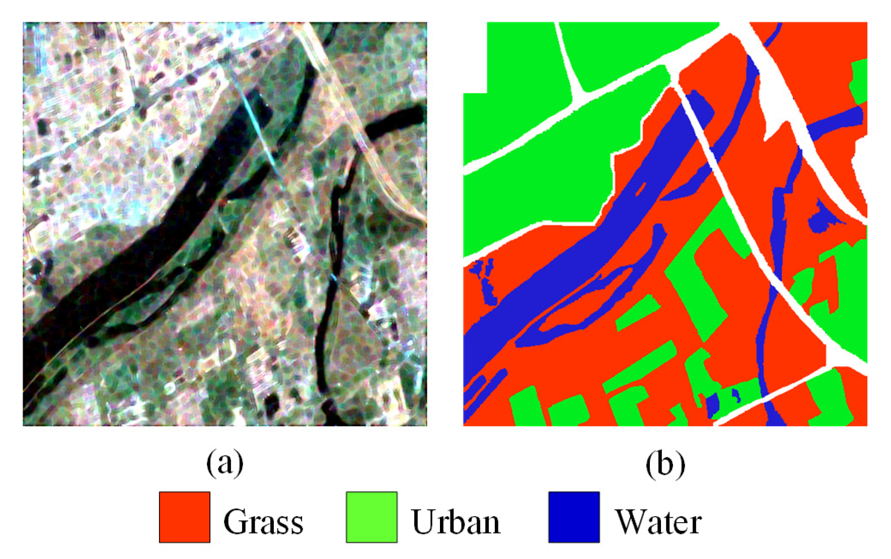
The Xi’an image dataset is a multi-look full polarimetric dataset acquired by Radarsat-2 satellite in C-band, which is shown in Figure 5a, and the corresponding ground truth is shown in Figure 5b. Its resolution is 8 × 8 m, and its size is 512 × 512 pixels. The Xi’an image contains three different terrain categories: grass, urban, and water.
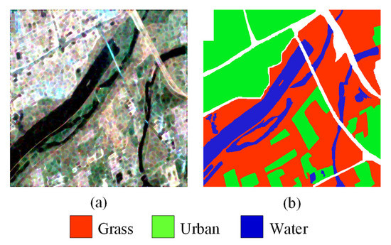
Figure 5.
Xi’an image. (a) Pseudo-RGB image. (b) Ground truth.
5.1.2. Oberpfaffenhofen Dataset
The Oberpfaffenhofen image was obtained from the E-SAR polarized SAR imaging system at the German Aerospace Center in Oberpfaffenhofen, Germany, as shown in Figure 6a, and the corresponding ground truth is shown in Figure 6b. The size of this image is about 1300 × 1200 pixels, including three different terrain categories: build-up area, wood land, and open area.
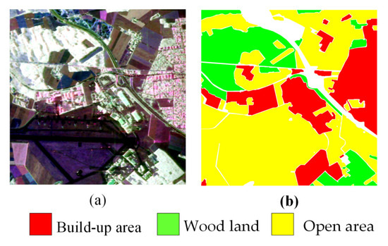
Figure 6.
Oberpfaffenhofen image. (a) pseudo-RGB image. (b) ground truth.
5.1.3. San Francisco Dataset
The San Francisco image is a C-band fully polarized SAR image, which is shown in Figure 7a, and the corresponding ground truth is shown in Figure 7b. The size of this image is about 900 × 1024 pixels, with five different terrain categories: low-density urban, water, vegetation, developed area, and high-density urban.
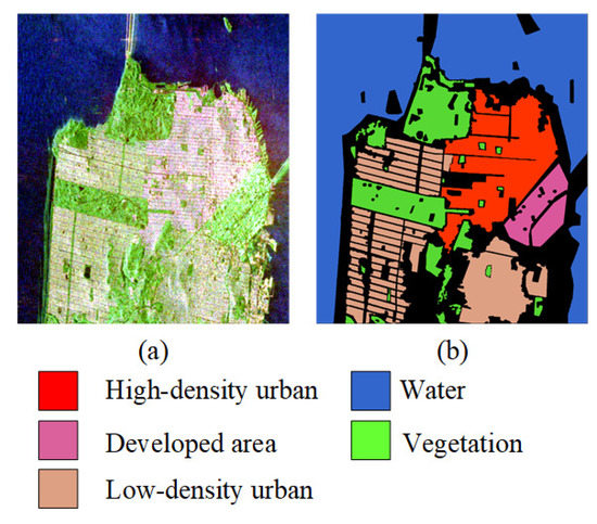
Figure 7.
San Francisco image. (a) pseudo-RGB image. (b) ground truth.
5.2. Parameter Setting
In our experiments, the neighborhood windows with 12 × 12 of each pixel are used as the input of CNN model, and in order to achieve better classification results, we needed to obtain as much global information as possible while ensuring a moderate amount of computation, so the input image was set as 128 × 128 for the SFCN model, which was obtained from the whole PolSAR image by the sliding window [39]. Through the same operation, the corresponding labeled samples were obtained from the ground truth. Meanwhile, the stride of the sliding window in the SFCN model was set to 32. The size and the stride of sliding window in the CV-SDFCN model are set to be the same as the SFCN model. In order to obtain a better approximate classification scheme and accelerate the convergence of the loss function, we use the Adam optimizer with 1 × 10 as the learning rate to optimize the objective function. The iteration and batch size of the model training are set to 300 and 30, respectively, which is an empirical choice after many experiments. In addition, in order to alleviate the problem of network overfitting, the dropout layer was introduced. The methods of SVM, Wishart and bagging were carried out on MATLAB R2016b; the others were implemented in python3.7 and Tensorflow 2.3.0 frameworks using NVIDIA RTX 3090.
5.3. Classification Results
5.3.1. Results for the Xi’an Dataset
In the experiment on the Xi’an dataset, 5% of the labeled samples were randomly selected for training. Table 1 provides the comparison of the OA value, Kappa coefficient, MIoU value, and the accuracy of each terrain on Xi’an images. As can be seen from Table 1, the classification results of Unet are better than other comparison methods. The OA values of Unet are about 9.49%, 12.94%, 9.51%, 3.55%, 5.02%, 3.18%, 0.74% higher than others, but the value of the CV-SDFCN method is very close to it. The Wishart classifier achieves a good accuracy in the water area of up to 94.37%. However, for grass and urban areas, the accuracies are only 84.01% and 81.87%, respectively, which leads the Kappa coefficient to be only 80.13%. Even though the SFCN model improves the accuracy of grass area to 92.17%, the accuracy of water is only 89.33%, which is worse than CVFCN. The OA, Kappa, and MIoU of CVFCN are about 1.86%, 1.68%, and 2% higher than SFCN, respectively, which demonstrates the significance of the phase information for PolSAR datasets. In particular, the accuracy of the water area of CV-SDFCN is about 6.05% higher than that of CVFCN. The main reason is that the performance of multi-scale features extracted by SDC blocks is superior to a single FCN model. To sum up, the classification results can prove the effectiveness of the CV-SDFCN model.

Table 1.
Classification accuracy of Xi’an dataset .
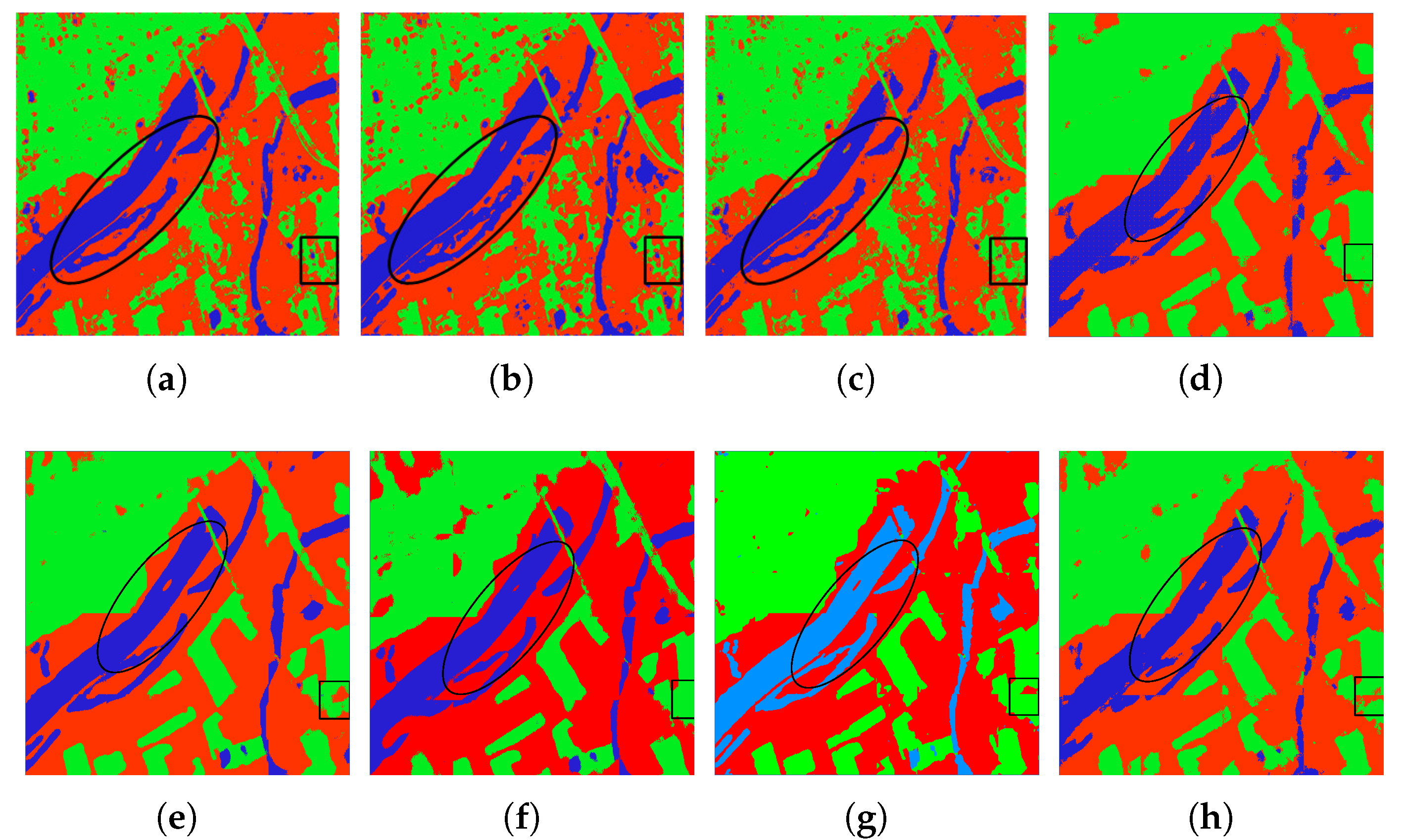
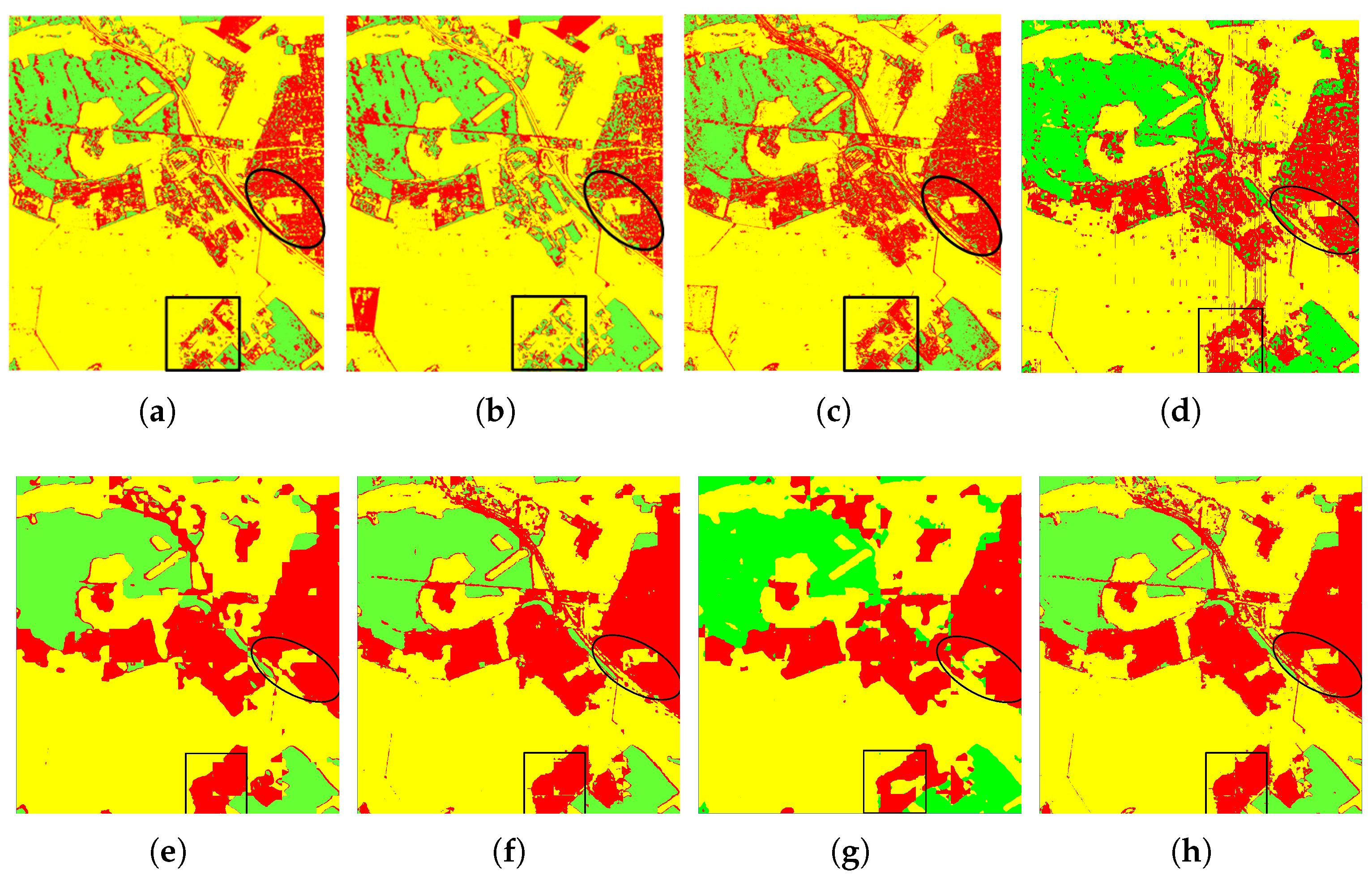
Figure 8 presents the classification results for all classification methods. We mark the prominent improvements with black ovals and rectangles. Figure 8a–c gives the classification results of SVM, Wishart, and Bagging, separately. We can clearly observe that the misclassifications of traditional classifiers are quite serious; in particular, the grass areas are seriously misclassified with urban areas. Figure 8d shows the classification results of CNN; it can be seen that CNN can clearly classify the outline of terrains, especially in the grass areas compared with the three formal algorithms. However, it still hardly distinguishes some pixels between the grass and urban, which has been highlighted by a blank rectangle. Figure 8e,f exhibit the classification results of SFCN and CVFCN, respectively. By contrast, we can distinctly see that the result for the FCN model is clearer and smoother than others, which has been highlighted by a black rectangle. We can also notice that the CVFCN model performs better in water areas, highlighted by a black oval, than the SFCN. This is mainly because the CVFCN model takes full advantage of the phase information of PolSAR datasets. Figure 8g,h present the results of Unet and our proposed method, which present better contextual consistency.
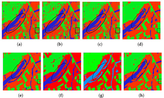
Figure 8.
Classification results for the Xi’an dataset with different methods. (a) SVM. (b) Wishart. (c) Bagging. (d) CNN. (e) SFCN. (f) CVFCN. (g) Unet. (h) CV-SDFCN.
5.3.2. Results of Oberpfaffenhofen Dataset
In order to demonstrate the effectiveness of the proposed method, the second experiment was carried on Oberpfaffenhofen, and 1% of labeled pixels were selected. Table 2 lists the comparison results of OA, Kappa, MIoU, and each terrain’s accuracy for different methods. It can be seen from Table 2 that the performance of CV-SDFCN is better than other methods under all the evaluation indices. The OA values of CV-SDFCN are about 11.71%, 14.6%, 8.1%, 7.02%, 3.18%, 1.79%, 2.54% higher than other comparison methods. The performances of SVM and Wishart were the worst. The Kappa coefficient of Wishart is only 67.59%. Bagging has a good result when classifying the wood area, but it has a few bad results in open areas and built-up areas. The accuracy of built-up areas in the SFCN model was 91.11%, which is about 9.85% higher than that of CNN. CVFCN makes a further improvement compared with SFCN. For CV-SDFCN, the OA, Kappa, and MIoU values are about 3.02%, 5.82%, and 8.22% higher than that for CVFCN, respectively, and the accuracy of open areas is as high as 99.12%. It can be seen that the method proposed in this paper is effective.
Table 2.
Classification accuracy of the Oberpfaffenhofen dataset .
The experimental results of different methods on the Oberpfaffenhofen dataset are shown in Figure 9. Figure 9a–c donate the virtual results of SVM, Wishart, and Bagging classification method, separately, which can be intuitively observed that the open areas and built-up areas are misclassified seriously. From Figure 9d, we can see that CNN model has some improvements compared with the traditional methods, but there are still lots of misclassification pixels. Figure 9e,f show the result maps of SFCN and CVFCN classification model, respectively. It can be clearly seen that the methods based on FCN model could classify the PolSAR image with better visual continuity than others, such as the areas which have been highlighted by black squares. Further, the classification result of CVFCN model is superior to SFCN, which attests to the significance of polarized information for PolSAR. Figure 9g is the result map of Unet, which is same to FCN. Figure 9h presents the result map of our method, from which it can be discovered that the misclassified pixels of CV-SDFCN is less than other compared methods.
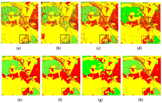
Figure 9.
Classification results of Oberpfaffenhofen dataset with different methods. (a) SVM. (b) Wishart. (c) Bagging. (d) CNN. (e) SFCN. (f) CVFCN. (g) Unet. (h) CV-SDFCN.
5.3.3. Results of San Francisco Dataset
We adopt the San Francisco dataset as the third experiment data to further verify the effectiveness of our method. 1% labeled pixels are selected for network training. Table 3 lists the classification accuracy of various algorithms on San Francisco dataset. From Table 3, it can be seen that the CV-SDFCN obtains better performance compared with other methods via OA value, Kappa coefficient and MIoU value. The OA value of CV-SDFCN is about 10.27%, 16.19%, 9.73%, 8.31%, 3.35%, 3.02%, 1.36% higher than other methods, respectively. We can come to a conclusion that the ability of feature extraction of traditional methods is inferior to deep learning methods, especially the Wishart classifier whose OA value is only 82.37%. The kappa coefficient and OA value of CNN are 85.69% and 90.25%, respectively, which are obviously higher than the formal ones. The OA value of SFCN is 95.21%, but the kappa coefficient is only 91.7%, and the accuracy of developed area is only 91.05%. Compared with SFCN model, the OA value of CVFCN is 95.54%, Kappa coefficient is 91.05% and MIoU value is 87.07% that is higher than SFCN. Furthermore, CV-SDFCN makes a great improvement compared with CVFCN, whose OA value, Kappa coefficient and MIoU value are 1.36%, 1.73% and 6.94% higher than Unet. It can be seen that the effectiveness of the method proposed in this paper can be certified.
Table 3.
Classification accuracy of San Francisco dataset .
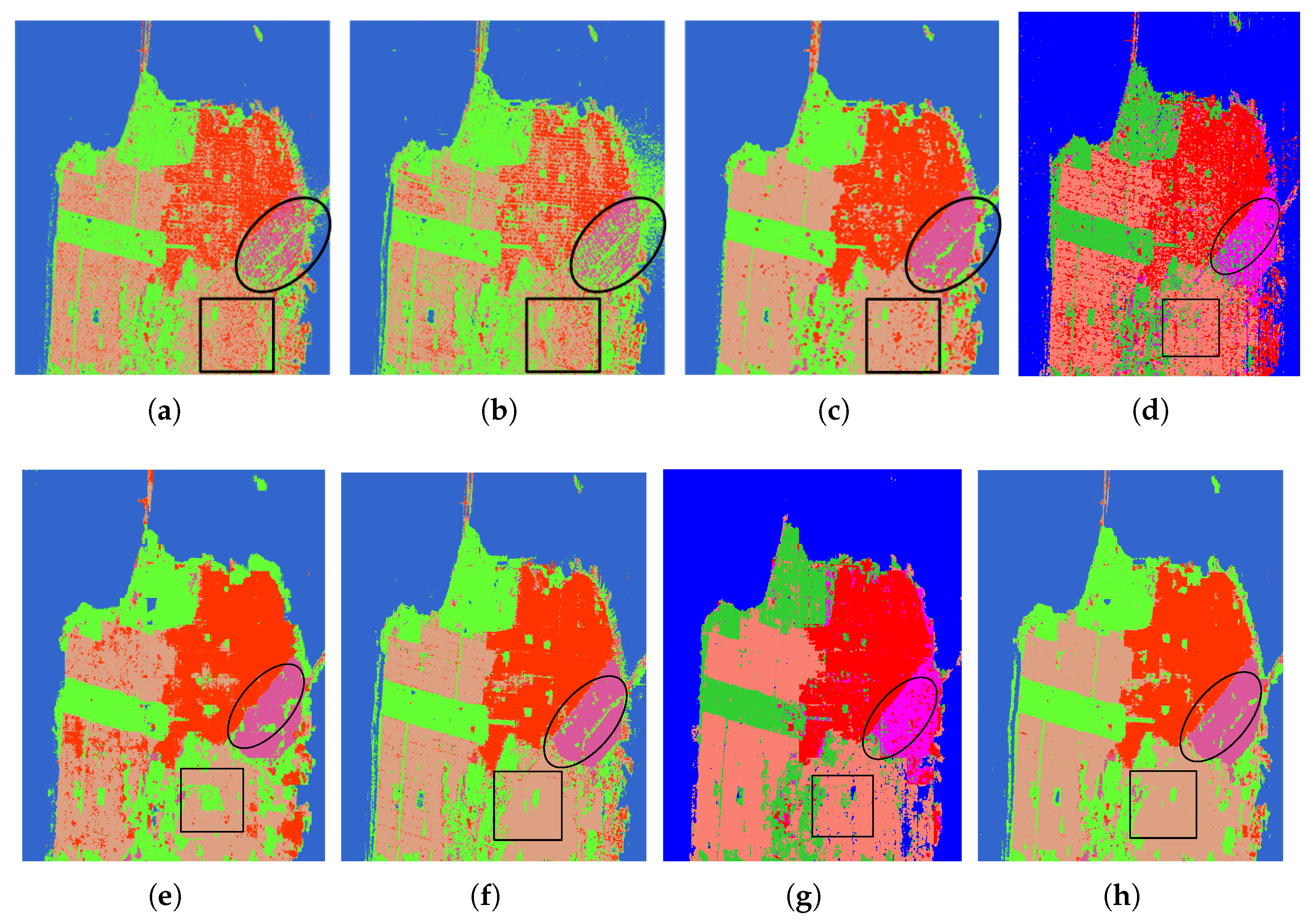
The classification results of different methods are shown in Figure 10a–h, in which the outstanding regions are marked with ovals and squares. Figure 10a–c show the visual classification results of SVM, Wishart, and Bagging. From Figure 10a,b, we can see that it is worst at distinguishing the developed and low-density areas that have been highlighted. The classification effect of Figure 10d is more clear compared with the formal methods, especially in low-density and developed areas; however, there are still some misclassified pixels. Figure 10g shows the result map of Unet; we can see that the classification effect in the vegetation area is very good compared with that of other methods. From Figure 10h, it can be seen that the effect of CV-SDFCN is further improved, especially in developed areas and low-density areas.
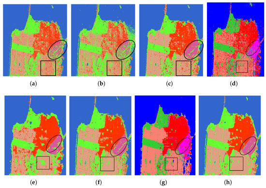
Figure 10.
Classification results of the San Francisco dataset with different methods. (a) SVM. (b) Wishart. (c) Bagging. (d) CNN. (e) SFCN. (f) CVFCN. (g) Unet. (h) CV-SDFCN.
5.3.4. Accuracy Boxplot
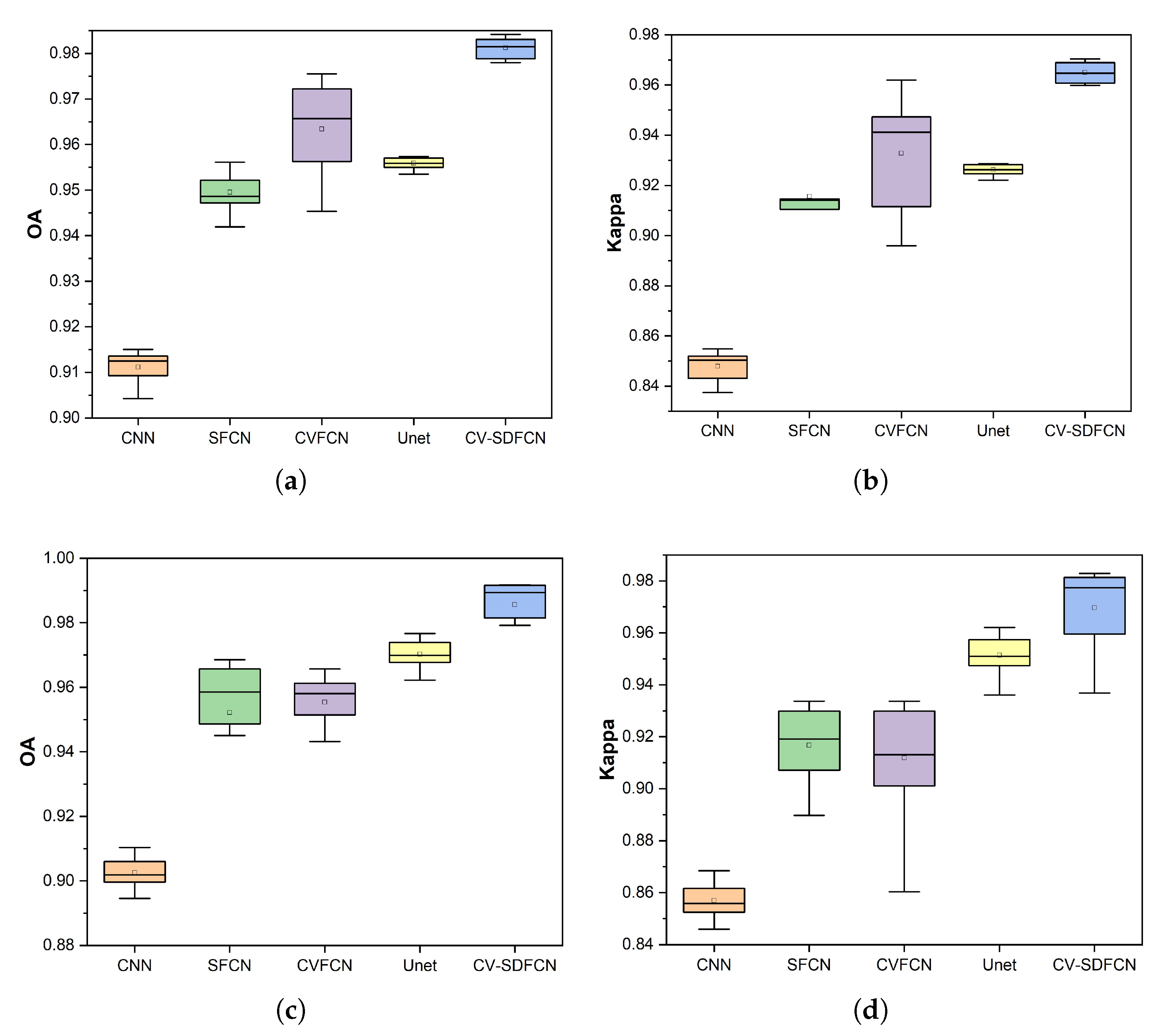
Tested on Oberpfaffenhofen and San Francisco datasets, accuracy boxplots of deep learning methods are shown in Figure 11. Different colored square represents different classification method. The box and horizontal line in colored square mean the average evaluation index. The boxplot in a more compact form means lower dispersion and stronger robustness. From Figure 11a,b, we can see that in the Oberpfaffenhofen dataset, the performance of our proposed structure is better than that of all other structures. What is more,the performance of Unet and CNN is more stable than that of other networks. The OA and Kappa values of CV-SDFCN are around 98% and 97%, respectively, which are far higher than those of CNN, which are 91% and 85%. It can be seen from Figure 11c,d that our network performance is also the best on the San Francisco dataset: the network performance is more stable, and the values of OA and Kappa are also the best. Therefore, the structure we proposed is more effective than all other structures.
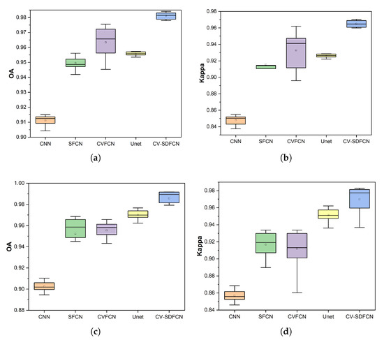
Figure 11.
Boxplots of OA and Kappa. (a) ESAR-OA. (b) ESAR-Kappa. (c) San-OA. (d) San-Kappa.
6. Conclusions
In order to effectively utilize the polarization characteristics of PolSAR data, we propose a multi-scale, fully convolutional network using stacked dilated convolutions in a complex-valued domain, which has been proved to be very effective. First, we constructed a stacked dilated convolution layer with different dilation rates to capture multi-scale image features. Meanwhile, sharing weights were utilized to reduce the computational burden. Then, in view of limited labeled samples for PolSAR images, the encoder and decoder operation of original FCN were reconstructed by a U-net. Finally, considering the significance of phase information for PolSAR images, the proposed method was established in a complex-valued domain rather than a real-valued domain. In order to verify the effectiveness and reliability of our proposed method, we carried out experiments on three PolSAR datasets, Xi’an, Oberpfaffenhofen, and San Francisco. By calculating the OA value, Kappa coefficient, and MIoU value, we proved that the performance of our method is better than that of several advanced classification methods. Furthermore, we draw the boxplot of Oberpfaffenhofen and San Francisco datasets to demonstrate the robustness and stability of our proposed method. Nevertheless, there are still some aspects to perfect in this paper. The proposed method is based on a single FCN model, but the image features extracted by a single model are usually not enough compared to those extracted by multiple models. In our future works, we shall associate different FCN models for PolSAR image classification.
Author Contributions
Conceptualization, W.X. and L.J.; Methodology, W.X. and L.J.; Software, W.X. and W.H.; Writing—Original Draft Preparation, W.X.; Writing—Review and Editing, W.X. and W.H.; Formal Analysis, W.H.; Validation, W.X. and W.H.; Data Curation, W.H.; Funding Acquisition, W.X. and W.H. All authors have read and agreed to the published version of the manuscript.
Funding
This research was funded by the National Natural Science Foundation of China (61901365, 61903168), the Natural Science Basic Research Plan in Shaanxi Province of China (2019JQ-377), and the Scientific Research Program Funded by Shaanxi Provincial Education Department (19JK0805).
Data Availability Statement
Not applicable.
Conflicts of Interest
The authors declare no conflict of interest.
References
- Krogager, E. New decomposition of the radar target scattering matrix. Electron. Lett. 2002, 26, 1525–1527. [Google Scholar] [CrossRef]
- Cloude, S.R.; Pottier, E. An entropy based classification scheme for land applications of polarimetric SAR. IEEE Trans. Geo. Remote Sens. 1997, 35, 68–78. [Google Scholar] [CrossRef]
- Freeman, A.; Durden, S.L. A three-component scattering model for polarimetric SAR data. IEEE Trans. Geosci. Remote Sens. 1998, 36, 963–973. [Google Scholar] [CrossRef] [Green Version]
- Xu, Q.; Chen, Q.; Yang, S.; Liu, X. Superpixel-Based Classification Using K Distribution and Spatial Context for Polarimetric SAR Images. Remote Sens. 2016, 8, 619. [Google Scholar] [CrossRef] [Green Version]
- Huynen, J.R. Phenomenological Theory of Radar Targets. Electromagn. Scatt. 1978, 653–712. [Google Scholar] [CrossRef] [Green Version]
- Lee, J.S.; Grunes, M.R.; Ainsworth, T.L.; Pottier, E.; Krogager, E.; Boerner, W.M. Quantitative comparison of classification capability: Fully-polarimetric versus partially polarimetric SAR. In Proceedings of the IEEE International Geoscience and Remote Sensing Symposium, Toronto, ON, Canada, 24–28 June 2002. [Google Scholar]
- Zhang, L.; Wang, X.; Li, M.; Moon, W.M. Classification of fully polarimetric SAR images based on ensemble learning and feature integration. In Proceedings of the Geoscience and Remote Sensing Symposium, Quebec City, QC, USA, 13–18 July 2014; pp. 2758–2761. [Google Scholar]
- Fukuda, S.; Hirosawa, H. Support vector machine classification of land cover: Application to polarimetric SAR data. In Proceedings of the IEEE 2001 International Geoscience and Remote Sensing Symposium (Cat. No. 01CH37217), Sydney, NSW, Australia, 9–13 July 2002. [Google Scholar]
- Okwuashi, O.; Ndehedehe, C.E.; Olayinka, D.N.; Eyoh, A.; Attai, H. Deep support vector machine for PolSAR image classification. Int. J. Remote Sens. 2021, 42, 6502–6540. [Google Scholar] [CrossRef]
- Liu, W.; Yang, J.; Li, P.; Han, Y.; Zhao, J.; Shi, H. A Novel Object-Based Supervised Classification Method with Active Learning and Random Forest for PolSAR Imagery. Remote Sens. 2018, 10, 1092. [Google Scholar] [CrossRef] [Green Version]
- Hong, F.; Kong, Y. Random Forest Fusion Classification of Remote Sensing PolSAR and Optical Image Based on LASSO and IM Factor. In Proceedings of the 2021 IEEE International Geoscience and Remote Sensing Symposium IGARSS, Brussels, Belgium, 11–16 July 2021; IEEE: New York, NY, USA, 2021; pp. 5048–5051. [Google Scholar]
- Hinton, G.; Deng, L.; Yu, D.; Dahl, G.E.; Kingsbury, B. Deep Neural Networks for Acoustic Modeling in Speech Recognition: The Shared Views of Four Research Groups. IEEE Signal Process. Mag. 2012, 29, 82–97. [Google Scholar] [CrossRef]
- Yang, B.; Liu, H.; Li, X. Learning Deep Direct-Path Relative Transfer Function for Binaural Sound Source Localization. IEEE/ACM Trans. Audio Speech Lang. Process. 2021, 29, 3491–3503. [Google Scholar] [CrossRef]
- Gu, J.; Wang, Z.; Kuen, J.; Ma, L.; Wang, G. Recent Advances in Convolutional Neural Networks. Pattern Recognit. 2018, 77, 354–377. [Google Scholar] [CrossRef] [Green Version]
- Cireşan, D.; Meier, U.; Schmidhuber, J. Multi-column Deep Neural Networks for Image Classification. In Proceedings of the 2012 IEEE Conference on Computer Vision and Pattern Recognition, Providence, RI, USA, 16–21 June 2012. [Google Scholar]
- Krizhevsky, A.; Sutskever, I.; Hinton, G. ImageNet Classification with Deep Convolutional Neural Networks. Adv. Neural Inf. Process. Syst. 2012, 25, 1097–1105. [Google Scholar] [CrossRef]
- Long, J.; Shelhamer, E.; Darrell, T. Fully Convolutional Networks for Semantic Segmentation. IEEE Trans. Pattern Anal. Mach. Intell. 2015, 39, 640–651. [Google Scholar]
- Garg, R.; Kumar, A.; Bansal, N.; Prateek, M.; Kumar, S. Semantic segmentation of PolSAR image data using advanced deep learning model. Sci. Rep. 2021, 11, 15365. [Google Scholar] [CrossRef] [PubMed]
- Protopapadakis, E.; Voulodimos, A.; Doulamis, A.; Doulamis, N.; Dres, D.; Bimpas, M. Stacked autoencoders for outlier detection in over-the-horizon radar signals. Comput. Intell. Neurosci. 2017, 2017, 5891417. [Google Scholar] [CrossRef] [PubMed]
- Volpi, M.; Tuia, D. Dense semantic labeling of sub-decimeter resolution images with convolutional neural networks. IEEE Trans. Geosci. Remote Sens. 2016, PP, 881–893. [Google Scholar]
- Jiao, L.; Hou, B.; Yang, S.; Liu, F. POL-SAR Image Classification Based on Wishart DBN and Local Spatial Information. IEEE Trans. Geosci. Remote Sens. 2016, 54, 3292–3308. [Google Scholar]
- Xie, W.; Xie, Z.; Zhao, F.; Ren, B. POLSAR image classification via Clustering-WAE classification model. IEEE Access 2018, 6, 40041–40049. [Google Scholar] [CrossRef]
- Xie, W.; Jiao, L.; Hou, B.; Ma, W.; Zhao, J.; Zhang, S.; Liu, F. POLSAR Image Classification via Wishart-AE Model or Wishart-CAE Model. IEEE J. Sel. Top. Appl. Earth Obs. Remote Sens. 2017, 10, 3604–3615. [Google Scholar] [CrossRef]
- Xie, W.; Ma, G.; Hua, W.; Zhao, F. Complex-Valued Wishart Stacked Auto-Encoder Network for Polsar Image Classification. In Proceedings of the IGARSS 2019—2019 IEEE International Geoscience and Remote Sensing Symposium, Yokohama, Japan, 28 July–2 August 2019; pp. 3193–3196. [Google Scholar] [CrossRef]
- Zhang, L.; Jiao, L.; Ma, W.; Duan, Y.; Zhang, D. PolSAR image classification based on multi-scale stacked sparse autoencoder. Neurocomputing 2019, 351, 167–179. [Google Scholar] [CrossRef]
- Liu, G.; Li, Y.; Jiao, L.; Chen, Y.; Shang, R. Multiobjective evolutionary algorithm assisted stacked autoencoder for PolSAR image classification. Swarm Evol. Comput. 2021, 60, 100794. [Google Scholar] [CrossRef]
- Hua, W.; Wang, X.; Zhang, C.; Jin, X. Attention-Based Multiscale Sequential Network for PolSAR Image Classification. IEEE Geosci. Remote Sens. Lett. 2022, 19, 1–5. [Google Scholar] [CrossRef]
- Bi, H.; Sun, J.; Xu, Z. A graph-based semisupervised deep learning model for PolSAR image classification. IEEE Trans. Geosci. Remote Sens. 2018, 57, 2116–2132. [Google Scholar] [CrossRef]
- Ren, S.; Zhou, F. Semi-Supervised Classification for PolSAR Data With Multi-Scale Evolving Weighted Graph Convolutional Network. IEEE J. Sel. Top. Appl. Earth Obs. Remote Sens. 2021, 14, 2911–2927. [Google Scholar] [CrossRef]
- Nie, W.; Huang, K.; Yang, J.; Li, P. A Deep Reinforcement Learning-Based Framework for PolSAR Imagery Classification. IEEE Trans. Geosci. Remote Sens. 2021, 60, 1–15. [Google Scholar] [CrossRef]
- Cheng, J.; Zhang, F.; Xiang, D.; Yin, Q.; Zhou, Y.; Wang, W. PolSAR Image Land Cover Classification Based on Hierarchical Capsule Network. Remote Sens. 2021, 13, 3132. [Google Scholar] [CrossRef]
- Chen, S.; Tao, C. PolSAR Image Classification Using Polarimetric-Feature-Driven Deep Convolutional Neural Network. IEEE Geosci. Remote Sens. Lett. 2018, 15, 627–631. [Google Scholar] [CrossRef]
- Cui, Y.; Liu, F.; Jiao, L.; Guo, Y.; Liang, X.; Li, L.; Yang, S.; Qian, X. Polarimetric Multipath Convolutional Neural Network for PolSAR Image Classification. IEEE Trans. Geosci. Remote Sens. 2021, 60, 1–18. [Google Scholar] [CrossRef]
- Geng, J.; Deng, X.; Ma, X.; Jiang, W. Transfer learning for SAR image classification via deep joint distribution adaptation networks. IEEE Trans. Geosci. Remote Sens. 2020, 58, 5377–5392. [Google Scholar] [CrossRef]
- Rostami, M.; Kolouri, S.; Eaton, E.; Kim, K. Deep transfer learning for few-shot SAR image classification. Remote Sens. 2019, 11, 1374. [Google Scholar] [CrossRef] [Green Version]
- Huang, Z.; Pan, Z.; Lei, B. Transfer learning with deep convolutional neural network for SAR target classification with limited labeled data. Remote Sens. 2017, 9, 907. [Google Scholar] [CrossRef] [Green Version]
- Huang, Z.; Dumitru, C.O.; Pan, Z.; Lei, B.; Datcu, M. Classification of large-scale high-resolution SAR images with deep transfer learning. IEEE Geosci. Remote Sens. Lett. 2020, 18, 107–111. [Google Scholar] [CrossRef] [Green Version]
- Wu, W.; Li, H.; Li, X.; Guo, H.; Zhang, L. PolSAR image semantic segmentation based on deep transfer learning—Realizing smooth classification with small training sets. IEEE Geosci. Remote Sens. Lett. 2019, 16, 977–981. [Google Scholar] [CrossRef]
- Li, Y.; Chen, Y.; Liu, G.; Jiao, L. A Novel Deep Fully Convolutional Network for PolSAR Image Classification. Remote Sens. 2018, 10, 1984. [Google Scholar] [CrossRef] [Green Version]
- Chen, Y.; Li, Y.; Jiao, L.; Peng, C.; Zhang, X.; Shang, R. Adversarial Reconstruction-Classification Networks for PolSAR Image Classification. Remote Sens. 2019, 11, 415. [Google Scholar] [CrossRef] [Green Version]
- Mohammadimanesh, F.; Salehi, B.; Mandianpari, M.; Gill, E.; Molinier, M. A new fully convolutional neural network for semantic segmentation of polarimetric SAR imagery in complex land cover ecosystem. ISPRS J. Photogramm. Remote Sens. 2019, 151, 223–236. [Google Scholar] [CrossRef]
- He, C.; Tu, M.; Xiong, D.; Liao, M. Nonlinear manifold learning integrated with fully convolutional networks for polSAR image classification. Remote Sens. 2020, 12, 655. [Google Scholar] [CrossRef] [Green Version]
- Mullissa, A.G.; Persello, C.; Stein, A. PolSARNet: A Deep Fully Convolutional Network for Polarimetric SAR Image Classification. IEEE J. Sel. Top. Appl. Earth Obs. Remote Sens. 2019, 12, 5300–5309. [Google Scholar] [CrossRef]
- Cao, Y.; Wu, Y.; Zhang, P.; Liang, W.; Li, M. Pixel-Wise PolSAR Image Classification via a Novel Complex-Valued Deep Fully Convolutional Network. Remote Sens. 2019, 11, 2653. [Google Scholar] [CrossRef] [Green Version]
- Mullissa, A.G.; Persello, C.; Reiche, J. Despeckling Polarimetric SAR Data Using a Multistream Complex-Valued Fully Convolutional Network. IEEE Geosci. Remote Sens. Lett. 2021, 19, 1–5. [Google Scholar] [CrossRef]
- Zhang, Z.; Wang, H.; Xu, F.; Jin, Y.Q. Complex-Valued Convolutional Neural Network and Its Application in Polarimetric SAR Image Classification. IEEE Trans. Geosci. Remote Sens. 2017, 55, 7177–7188. [Google Scholar] [CrossRef]
- Zhao, F.; Tian, M.; Xie, W.; Liu, H. A New Parallel Dual-Channel Fully Convolutional Network via Semi-Supervised FCM for PolSAR Image Classification. IEEE J. Sel. Top. Appl. Earth Obs. Remote Sens. 2020, 13, 4493–4505. [Google Scholar] [CrossRef]
- Ulaby, F.T.; Elachi, C. Radar Polarimetry for Geoscience Applications. Geocarto Int. 1990, 5, 376. [Google Scholar] [CrossRef]
- Lee, J.S.; Grunes, M.R. Feature Classification Using Multi-look Polarimetric SAR Imagery. In Proceedings of the International Geoscience and Remote Sensing Symposium, Houston, TX, USA, 26–29 May 1992; pp. 77–79. [Google Scholar]
- Yu, F.; Koltun, V. Multi-Scale Context Aggregation by Dilated Convolutions. arXiv 2015, arXiv:1511.07122. [Google Scholar]
- Tseng, K.K.; Sun, H.; Liu, J.; Li, J.; Ip, W.H. Image semantic segmentation with an improved fully convolutional network. Soft Comput. 2020, 24, 8253–8273. [Google Scholar] [CrossRef]
- Zhao, W.; Fu, Y.; Wei, X.; Wang, H. An Improved Image Semantic Segmentation Method Based on Superpixels and Conditional Random Fields. Appl. Sci. 2018, 8, 837. [Google Scholar] [CrossRef] [Green Version]
- Chiheb, T.; Olexa, B.; Dmitriy, S.; Sandeep, S.; João Felipe, S.; Soroush, M.; Negar, R.; Yoshua, B.; Christopher, J.P. Deep Complex Networks. arXiv 2017, arXiv:1705.09792. [Google Scholar]
- Schuster, R.; Wasenmüller, O.; Unger, C.; Stricker, D. SDC - Stacked Dilated Convolution: A Unified Descriptor Network for Dense Matching Tasks. In Proceedings of the IEEE Conference on Computer Vision and Pattern Recognition (CVPR), Long Beach, CA, USA, 15–20 June 2019. [Google Scholar]
- Wang, P.; Chen, P.; Yuan, Y.; Liu, D.; Huang, Z.; Hou, X.; Cottrell, G. Understanding Convolution for Semantic Segmentation. In Proceedings of the 2018 IEEE Winter Conference on Applications of Computer Vision (WACV), Lake Tahoe, NV, USA, 12–15 March 2018; pp. 1451–1460. [Google Scholar] [CrossRef] [Green Version]
- Fisher, Y.; Vladlen, K.; Thomas, A.F. Dilated Residual Networks. arXiv 2017, arXiv:1705.09914. [Google Scholar]
- Wang, S.; Hu, S.Y.; Cheah, E.; Wang, X.; Wang, J.; Chen, L.; Baikpour, M.; Ozturk, A.; Li, Q.; Chou, S.H. U-Net Using Stacked Dilated Convolutions for Medical Image Segmentation 2020. arXiv 2020, arXiv:2004.03466. [Google Scholar]
- Gang, H.; Xianlin, L. Semantic segmentation of polarimetric synthetic aperture radar images based on deep learning. Scence Surv. Mapp. 2019, 1168, 042008. [Google Scholar]
- Ronneberger, O.; Fischer, P.; Brox, T. U-Net: Convolutional Networks for Biomedical Image Segmentation. arXiv 2015, arXiv:1505.04597. [Google Scholar]


Publisher’s Note: MDPI stays neutral with regard to jurisdictional claims in published maps and institutional affiliations. |
© 2022 by the authors. Licensee MDPI, Basel, Switzerland. This article is an open access article distributed under the terms and conditions of the Creative Commons Attribution (CC BY) license (https://creativecommons.org/licenses/by/4.0/).