Arctic Multiyear Ice Areal Flux and Its Connection with Large-Scale Atmospheric Circulations in the Winters of 2002–2021

Abstract

Arctic sea ice, especially the multiyear ice (MYI), is decreasing rapidly, partly due to melting triggered by global warming, in turn partly due to the possible acceleration of ice export from the Arctic Ocean to southern latitudes through identifiable gates. In this study, MYI and total sea ice areal flux through six Arctic gateways over the winters (October–April) of 2002–2021 were estimated using daily sea ice motion and MYI/total sea ice concentration data. Inconsistencies caused by different data sources were considered for the estimate of MYI flux. Results showed that, there is a slight declining trend in the Arctic MYI areal flux over the past two decades, which is attributable to the decrease in MYI concentration. Overall speaking, MYI flux through Fram Strait accounts for ~87% of the Arctic MYI outflow, with an average of ~325.92 × 10³ km² for the winters of 2002–2021. The monthly MYI areal flux through Fram Strait is characterized with a peak in March (~55.56 × 10³ km²) and a trough in April (~40.97 × 10³ km²), with a major contribution from MYI concentration. The connections between sea ice outflow and large-scale atmospheric circulations such as Arctic Oscillation (AO), North Atlantic Oscillation (NAO) and Dipole Anomaly (DA) were investigated. High correlation coefficients (CCs) were found in winter months such as January and February. While AO and NAO (especially NAO) exhibited generally weak correlations with the MYI/total sea ice flux, DA presented strong correlations with the areal flux, especially for MYI (CC up to 0.90 in January). However, the atmospheric circulation patterns are sometimes not fully characterized by the specific indices, which could have different effects on sea ice flux and its correlation with the atmospheric indices.

1. Introduction

In the Arctic Ocean, sea ice regulates the heat, moisture, momentum, and material exchanges between the ocean and atmosphere [1]. As one of the most sensitive and important indicators of climate change, Arctic sea ice profoundly affects the global climate system with a positive feedback [2,3,4,5]. Since the 1980s, the Arctic sea ice extent has declined by over 4%/decade [6], while that of the multiyear ice (MYI), i.e., sea ice that survives at least one summer melt, has reduced at a higher rate of 9–15%/decade [7,8,9]. A considerable part of the MYI that originally occupied two-thirds of the Arctic Ocean has been replaced by first-year ice (FYI) [10,11]. The more FYI dominates in the Arctic Ocean, the more vulnerable sea ice is to external forcings such as wind, waves, and currents.

Apart from melting, another possible cause for the recent decline in Arctic sea ice (particularly the MYI) would be the export southward to nearby open seas through specific gateways. It was found that Fram Strait is the major flux gate for the sea ice export from the Arctic Ocean [12,13,14]. Sea ice export through Fram Strait provides the largest component of freshwater for the Greenland-Iceland-Norwegian (GIN) Sea [15,16] and potentially modulates the properties of dense water in the Nordic Seas [17]. Moreover, sea ice outflow via Fram Strait is a primary constituent of the mass balance of the Arctic Ocean [18]. Notably, total sea ice transport through other gateways is receiving more and more attention despite their relatively small flux [19,20,21,22,23]. Nevertheless, less attention has been paid to the MYI flux, which could have a predominant impact on the Arctic ice mass balance due to the larger thickness of MYI. The variability of Arctic MYI flux and the mechanisms behind are of great scientific interest, however, have been rarely investigated. On one hand, the contribution of MYI areal flux to the Arctic MYI area decreased and the correlation with the Arctic sea ice volume flux is still unclear. On the other hand, a consistent long-term MYI dataset is needed for such investigation, while its uncertainty and inconsistency limit its application. Inconsistencies caused by different data sources (scatterometers or radiometers) may have a significant impact on the MYI concentration as well as the MYI flux estimates. For instance, the Ku-band scatterometer (e.g., QSCAT) is more effective than the C-band scatterometer (e.g., ASCAT) in identifying MYI from FYI due to the stronger volume scattering at Ku-band [24]. Nonnegligible differences in the MYI concentration and the MYI flux are expected and should be taken into account when estimated from the two scatterometer data. A recent study presents the MYI areal flux of the past 18 years [25], yet it does not account for the data inconsistency and focuses on Fram Strait only.

Arctic sea ice flux and its connection with large-scale atmospheric circulations have been investigated in several studies [26,27,28,29]. Atmospheric patterns such as Arctic Oscillation (AO) [30], North Atlantic Oscillation (NAO) [31], and Dipole Anomaly (DA) [32] are found to be correlated with total sea ice flux to different extents [33,34,35,36,37,38,39]. While the interaction between ice and atmosphere appears clearer, it remains vague how the large-scale atmospheric circulation influences the flux of thicker sea ice, i.e., MYI.

In this study, daily MYI as well as total sea ice areal flux through six Arctic fluxgates (Figure 1) for the winters (October–April) of 2002–2021 were estimated using satellite observations. Systematic bias in the MYI flux estimates caused by different data sources was removed. Spatial and temporal variabilities of total sea ice and MYI flux were analyzed. Their links with large-scale atmospheric circulations were further explored using indices derived from atmospheric reanalysis products. This paper is organized as follows. Section 2 introduces the datasets used in this study. Section 3 describes the methods and procedures on estimating total sea ice and MYI areal flux. Section 4 and Section 5 focus on the results and discussions, respectively. Section 6 presents the conclusions.

2. Data

Sea ice concentration and ice drift data retrieved from satellite observations were used to estimate the sea ice areal flux through the six water gateways in the Arctic (Figure 1). In addition, atmospheric reanalysis data and the large-scale atmospheric indices calculated from the former were used to investigate their links with the ice areal flux.

2.1. Sea Ice Concentration Data

The sea ice concentration data used for calculating the MYI and total sea ice areal flux were retrieved from Environment Canada’s Ice Concentration Extractor (ECICE) [40], which combines active and passive microwave remote sensing observations. The ECICE algorithm [40] builds upon a linear mixing model that decomposes each input radiometric observation into contributions from each surface type (i.e., open water, FYI, and MYI in our case), weighted by the concentration of each surface type within the grid. It obtains the optimal sea ice type concentration estimates by minimizing the sum of the squared difference between the observed and expected values based on the linear mixing model. Instead of employing a single typical radiometric value for each surface type in the linear mixing model, the algorithm uses the probability density distribution for each surface type and a Monte Carlo simulation to derive a large number of possible solutions. Medians of all the possible solutions are regarded as the final optimal solution [40].

ECICE algorithm was used in this study by combining scatterometer and passive microwave radiometer observations. The scatterometer included observations from SeaWinds onboard NASA’s QuikSCAT satellite (QSCAT) and ESA’s Advanced Scatterometer (ASCAT), both were accessed from the French Research Institute for Exploitation of the Sea (IFREMER). Passive microwave radiometer data included the Advanced Microwave Scanning Radiometer for EOS/2 (AMSR-E/2) and the Special Sensor Microwave Imager/Sounder (SSMIS), were acquired from the National Snow and Ice Data Center (NSIDC). Input data to ECICE covering different time ranges are shown in

Table 1. Information of the active and passive microwave observations input to ECICE for different periods.

Winter (October–April) of Years	ECICE Input Data	Input Parameters
2002–2009	QSCAT, AMSR-E	σ0hh, σ0vv, Tb37h, Tb37v
2009–2011	ASCAT, AMSR-E	σ0, Tb19h, Tb37h, GR37v19v
2011–2012	ASCAT, SSMIS	σ0, Tb19h, Tb37h, GR37v19v
2012–2021	ASCAT, AMSR2	σ0, Tb19h, Tb37h, GR37v19v

Note: σ⁰_hh and σ⁰_vv are backscatter of QSCAT in the horizontal and vertical polarization channels, respectively. σ⁰ denotes the backscatter of ASCAT. Tb_37h and Tb_37v correspond to the brightness temperature in the horizontal and vertical polarization from the 37-GHz radiometer, respectively. GR_37v19v represents the gradient ratio of brightness temperature [41] between 37-GHz and 19-GHz in the vertical polarization.

. The retrieved MYI and total sea ice concentration estimates are generated in a polar stereographic projection with a grid spacing of 12.5 km.

2.2. Sea Ice Motion Data

Daily gridded ice motion data from 2002 to 2021 were obtained from NSIDC (https://nsidc.org/data/NSIDC-0116/versions/4, accessed on 8 June 2022). The data are based on observations from the Advanced Very High-Resolution Radiometer (AVHRR), AMSR-E, Scanning Multichannel Microwave Radiometer (SMMR), Special Sensor Microwave/Imager (SSM/I), SSMIS, International Arctic Buoy Program (IABP) buoys and the US National Centers for Environmental Prediction/National Center for Atmospheric Research (NCEP/NCAR) reanalysis forecasts. By combining all the above sources via an optimal interpolation scheme, the newest sea ice motion data (Version 4) is provided with an EASE-grid with a spatial spacing of 25 km and made available for a long period from 1978 to 2021 [42]. The sea ice motion fields were resampled to a grid spacing of 12.5 km with the nearest neighbor interpolation method in order to match the ice concentration products from ECICE, hence calculating the ice flux.

2.3. Atmospheric Data

To explore the connection between sea ice areal flux and atmospheric circulation patterns, atmospheric variables from ERA5 and three atmospheric indices, AO, NAO, and DA, were examined in this study.

ERA5 represents the fifth generation of the European Centre for Medium-Range Weather Forecasts (ECMWF) atmospheric reanalysis of the global climate covering the period from January 1950 to the present. This new reanalysis product replaces the ERA-Interim (spanning 1979 onwards) and provides hourly estimates of a number of oceanic, land, and atmospheric climate variables with an enhanced horizontal resolution of 31 km [43,44]. The used ERA5 data was obtained from the Copernicus Climate Change Service (C3S). The hourly 2 m surface air temperature on single levels with a resolution of 0.25° from ECMWF ERA5 was used to correct the MYI concentrations which are suggested to have been underestimated (Section 3.1). In addition, the monthly sea level pressure (SLP) and 10 m wind (single level reanalysis with a resolution of 0.25°) were used to analyze the possible correlation between sea ice areal flux and DA index (Section 4.4).

AO is generally defined as the leading principal component of Northern Hemisphere SLP variability on the basis of empirical orthogonal function (EOF) analysis [30], which can be characterized as an exchange of atmospheric mass between the Arctic Ocean and the surrounding zonal ring centered ~45°N [36]. When AO is in the positive phase, the Icelandic low region presents anomalously low SLP, and the Beaufort Sea High (BSH) is weakened, resulting in a cyclonic circulation anomaly and hence facilitating the sea ice export through Fram Strait. When AO is in its negative phase, the anticyclonic anomaly in the sea ice flow is expected, which inhibits the sea ice export [45]. The AO index is available from the Climate Prediction Center of the National Oceanic Atmospheric Administration (NOAA, https://www.cpc.ncep.noaa.gov/products/precip/CWlink/, accessed on 8 June 2022).

NAO is known as a phenomenon associated with the dominant mode of North Atlantic atmospheric variability and is related to the simultaneous weakening and strengthening between the Azores high and Icelandic low [31]. The positive NAO phase is related to an intense Icelandic low and a strong Azores high, during which the SLP gradient across Fram Strait strengthens, causing strong northerly winds and hence increases the sea ice outflow [33,34]. Conversely, the negative NAO mode demonstrates the opposite SLP anomalies, leading to a reduced sea ice export through Fram Strait. The NAO index was obtained from the Climate Prediction Center of NOAA (https://www.cpc.ncep.noaa.gov/products/precip/CWlink/, accessed on 8 June 2022).

DA is the second-leading mode based on the EOF analysis of monthly mean SLP north of 70°N during the winter season and accounts for 13% of the variance in sea ice motion [32,46]. It is exhibited with two anomalous SLP centers. One is situated between the Kara Sea and the Laptev Sea, the other is occupied from the Canadian Archipelago through Greenland and extends to the Nordic seas. During the positive DA phase, the negative SLP anomalies appear in the Kara Sea-Laptev Sea and the positive SLP anomalies occur over the Canadian Archipelago. While during the negative DA phase, the SLP anomalies demonstrate an opposite scenario. The DA index used in this study was calculated using the afore-mentioned atmospheric reanalysis following the details described in [32].

3. Methods

MYI as well as the total sea ice areal flux for the winters of 2002–2021 were estimated following the methods described in the flowchart (Figure 2). Firstly, MYI and total sea ice concentration were retrieved from the ECICE algorithm with combinations of scatterometer and radiometer data as described above. For the MYI concentration, two correction schemes were applied, one to restore the underestimated and the other to restore the overestimated MYI concentration (Section 3.1). On this basis, total sea ice and the improved MYI concentration were then used to calculate the areal flux in combination with sea ice drift data (Section 3.2). Afterward, systematic bias caused by different data sources was obtained and removed from the derived MYI areal flux (Section 3.3).

3.1. Improvement in the Retrieval of MYI Concentration

Total sea ice concentration and partial concentration of different ice types (e.g., MYI concentration) can be retrieved from the ECICE algorithm [40] by combining both active or passive microwave remote sensing observations. On account of the discontinuity of the microwave scatterometer and radiometer data, four sets of ECICE input data and two sets of parameters corresponding to the QSCAT (2002–2009) and ASCAT (2009–2021) periods (Table 1) were used to retrieve total sea ice and MYI concentration. Both sets of input parameters have been used in previous studies for MYI concentration estimation though have slightly different performances [47,48,49]. To account for the differences induced by using the four sets of input data, results were later normalized to the same level as that in the QSCAT period (Section 3.3).

Total sea ice concentration can be retrieved quite reliably from ECICE [47,49] and thus was directly used for the ice areal flux calculation. In comparison, MYI concentration could have relatively low accuracy due to the disruption of a similar radiometric signature but from different ice types [50,51]. It has been found that during warm spells in the autumn and spring seasons (e.g., in October), MYI could be misclassified as FYI when snow wetness over MYI develops. Anomalous changes in the brightness temperature (sharp increase) and radar backscatter (sudden decrease) from the MYI surface are observed for a period of 10 days, resulting in a similar microwave signature as those from the FYI surface thus resulting in an underestimation of MYI concentration from ECICE [47,52]. On the other hand, during warm spells in spring (e.g., in April), FYI could be misidentified as MYI when snow metamorphism occurs over FYI. Under this condition, the brightness temperature from the FYI surface decreases, and the backscatter increases to values close to those of the MYI, leading to overestimated MYI estimates [48]. The correction for the former cases is based on air temperature records and MYI concentration daily changes, which help to determine the starting and ending date of the correction as well as the corrected MYI concentration [47,52]. For the latter situation, the correction builds upon the sea ice drift records of the Arctic. It considers the temporal evolution of MYI and constrains it with the tolerance of ice motion [48]. Note that when implementing the latter correction procedure, we adjusted the original threshold for defining the MYI domain from 15% to 20% to account for the impact of different spatial resolutions since a resolution of 4.45 km was used in [48] while 12.5 km is used in this study.

With the two correction schemes applied to the MYI concentration retrieval from ECICE, we derived the improved MYI concentration, which was then used for the flux calculation.

3.2. Areal Flux Calculation

Sea ice areal flux of the six gates was calculated using the aforementioned sea ice concentration and drift data. For each fluxgate, a transect across the gate was predefined (red lines in Figure 1). The six transects span a length of 112 km to 473 km (

Table 2. Length and grid numbers of each gate.

Fluxgates	Length (km)	Number of Grids
Fram Strait	455	36
Svalbard–Franz Josef (S–FJ)	314	25
Franz Josef–Severnaya Zemlya (FJ–SZ)	473	38
Bering Strait	132	11
Lanscater Sound	112	9
North Gate	314	25

). As well, all the flux calculations were performed on a polar stereographic grid with a spatial spacing of 12.5 km.

Daily areal flux across each gate can be calculated with the following equation [45]:

$$\mathrm{F}=\mathit{G}{\displaystyle \sum }_{\mathit{i}=1}^{\mathit{N}}{\mathit{M}}_{\mathit{i}}{\mathit{C}}_{\mathit{i}} \left(\mathit{i}=1,2,\dots ,\mathit{N}\right)$$

(1)

where M_i is the ice motion component perpendicular to the gate, ${\mathit{C}}_{\mathit{i}}$ is the sea ice concentration (when ${\mathit{C}}_{\mathit{i}}$ is the total sea ice and MYI concentration, F is the total sea ice and MYI areal flux, respectively). G is the grid size of 12.5 km, whereas i represents the individual grid along the transect of each flux gate.

Daily and monthly sea ice areal flux of all the six gates were calculated for the winters of 2002–2021. Note that positive flux refers to the export of Arctic sea ice from the higher-latitude Arctic Ocean into the lower-latitude adjoining seas while the negative one refers to the opposite scenario.

3.3. Normalization of Preliminary Results

Inconsistencies resulting from using the afore-mentioned four sets of ECICE input data influence the MYI concentration retrieval [49], which eventually leads to inconsistent estimates in MYI areal flux for the different years. As shown in Figure 3, there are clear differences in the MYI areal flux calculated from the four sets of data sources during the overlapping periods. The largest discrepancy occurs in the winters of 2007–2009, when different scatterometer data are used (QSCAT-AMSRE and ASCAT-AMSRE). The average bias of the wintertime Arctic MYI areal flux calculated from the QSCAT-AMSRE and ASCAT-AMSRE dataset reaches 111.60 × 10³ km², whereas the bias induced by the different radiometers is much smaller, the average of which amounts to 17.95 × 10³ km² and 7.69 × 10³ km² for the winters of 2009–2011 (ASCAT-AMSRE and ASCAT-SSMIS) and 2012–2014 (ASCAT-SSMIS and ASCAT-AMSR2), respectively.

To quantify the discrepancies between the datasets, we calculated the areal flux with the MYI concentration from each pair of the datasets during the overlapping periods. For example, daily MYI areal flux is calculated, respectively, using the MYI concentration from the QSCAT-AMSRE and ASCAT-AMSRE microwave observations for the overlapping winters of 2007–2009. Two sets of monthly MYI flux and their differences are then obtained for the two winters (2007/2008 and 2008/2009). The average of the monthly differences for the same month of the two winters is taken as the monthly bias between the two datasets. The sum of the bias of each winter month (October–April) is regarded as the bias of the entire winter. Based on the bias between each two datasets (see Table 1 for the microwave observations used in ECICE), the MYI areal flux of all the years was adjusted to a level consistent with those over the QSCAT-AMSRE period (i.e., adjusting the results of 2009–2021 to those of 2002–2009). The QSCAT-AMSRE dataset was selected as the reference due to the following two factors. On one hand, Ku-band scatterometer (e.g., QSCAT) is expected to have a better performance than C-band scatterometer (e.g., ASCAT) in classifying MYI from seasonal ice due to their higher sensitivity to the volumetric scattering which is common in MYI floes [24]. On the other hand, previous studies have demonstrated that MYI concentration estimates are reliable when the QSCAT-AMSRE inputs are adopted to ECICE [48,49,52].

4. Results

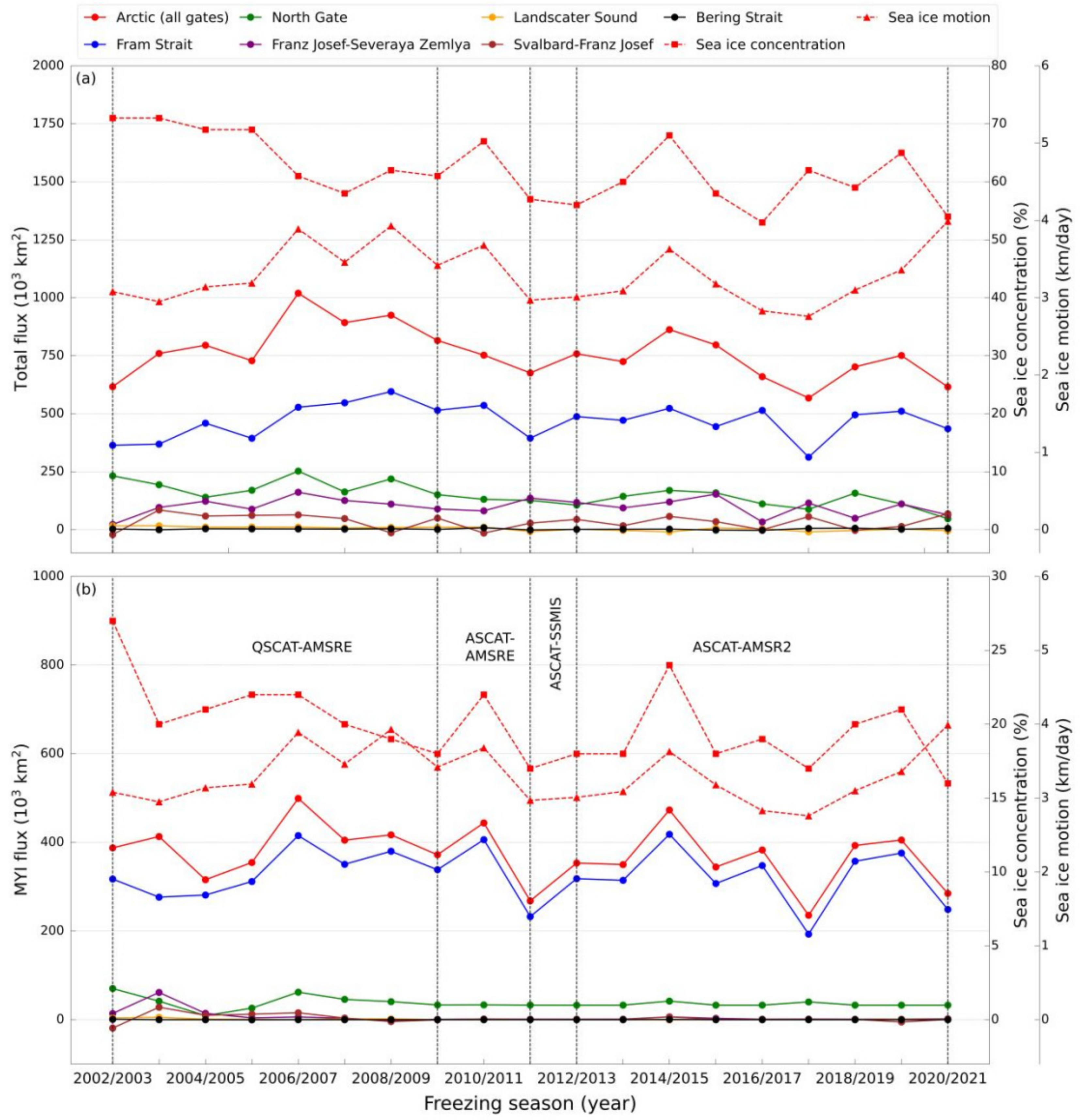
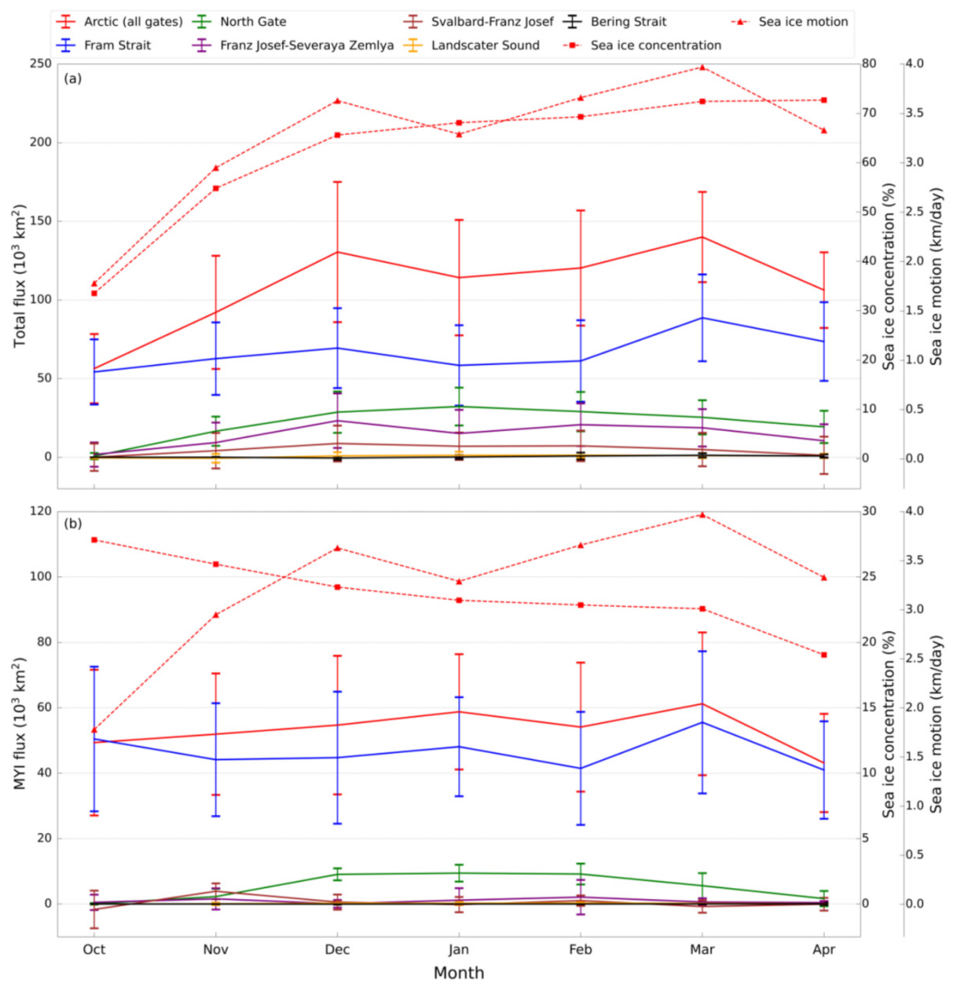
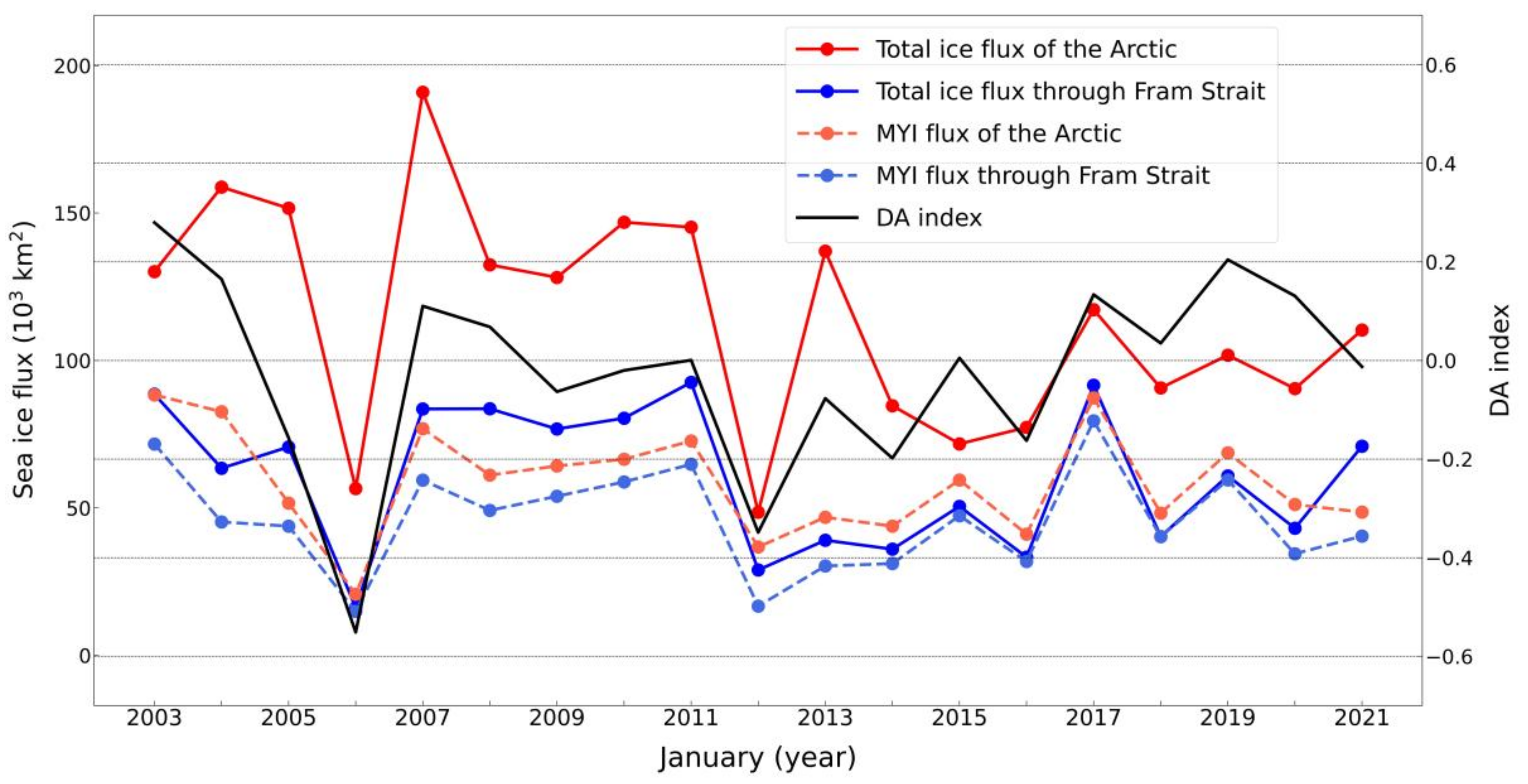
4.1. Time Series of Total Sea Ice and MYI Areal Flux

The total sea ice areal flux as well as the MYI flux (after normalization) for the winters of 2002–2021 are presented in Figure 4. Overall, a weak decreasing trend (−9.8%/decade) in the Arctic total sea ice areal flux is observed over the past two decades (Figure 4a), which seems to be associated with the decrease in the total sea ice concentration (−9.8%/decade, p < 0.01). With regard to the Arctic MYI flux, there is also a slight negative trend (−9.2%/decade) (Figure 4b), which is related to the decreasing MYI concentration (−12.5%/decade, p < 0.05). Moreover, the inter-annual variabilities in the MYI flux of the Arctic and through Fram Strait are significant, with a standard deviation of about 59.36 × 10³ km² and 71.66 × 10³ km², respectively.

While the Arctic total sea ice areal flux is 759.02 × 10³ km² on average in winter, more than half of this amount (about 62%) is advected through Fram Strait (approximately 468.30 × 10³ km²) (Figure 4a). In comparison, the areal flux through the other gates is relatively small, especially from Lanscater Sound and Bering Strait, whose total sea ice flux is nearly zero. Notably, the areal flux through Fram Strait is much larger than that via FJ–SZ (winter mean total flux is about 99.40 × 10³ km²), although the latter gate is wider (Table 2). This is because the Transpolar Drift carries sea ice from the Arctic Basin through Fram Strait, but not through FJ–SZ. Regarding the MYI outflow (Figure 4b), the mean areal flux for the nineteen winters through Fram Strait and of the Arctic amount to approximately 325.92 × 10³ km² and 373.72 × 10³ km², respectively. The MYI flux via Fram Strait occupies the majority of the Arctic MYI flux, with an average percentage reaching around 87%. The second largest contribution of MYI outflow (about 10%) occurs in North Gate. MYI flux through the other four fluxgates is close to zero except for the winter before 2007/2008.

In addition to the inter-annual variation of sea ice areal flux, the monthly variability in the total sea ice and MYI flux were also examined and presented in Figure 5a,b, respectively.

As depicted in Figure 5a, the total sea ice areal flux through Fram Strait and of the Arctic shows a clear increasing trend from October to December, and maintains a stable state from January to March, followed by a significant decline in April. Overall, there are slight growing trends throughout the winter months (5.6%/month through Fram Strait and 7.8%/month of the Arctic), which is attributed to the positive trends both in the total sea ice concentration and ice motion (8.9%/month in total sea ice concentration and 7.4%/month in ice motion). As for the MYI flux (Figure 5b), there are subtle increasing trends from October to March through Fram Strait and of the Arctic, while a significant decrease in April is observed. Overall, there are virtually negligible monthly trends in the MYI flux from October to April, which is due to the balanced effects related to a decreasing MYI concentration (−5.2%/month, p < 0.01) and an increasing sea ice drift (7.4%/month). In comparison, the percentage of the Arctic monthly MYI flux from the total sea ice flux decreases at a rate of −11.0%/month from October to April. Meanwhile, we note that larger standard deviations usually occur in the months with a greater areal flux, which is more distinct for the MYI outflow.

The smallest total sea ice areal flux via each fluxgate appears in October. While the largest total sea ice outflow through Fram Strait and of the Arctic both occur in March (Figure 5a), with an average maximum flux of 88.68 × 10³ km² and 140.01 × 10³ km², respectively. For the MYI (Figure 5b), the areal flux through Fram Strait and of the Arctic both peaks in March (55.56 × 10³ km² and 61.23 × 10³ km², respectively), and drops into the troughs in April (40.97 × 10³ km² and 43.13 × 10³ km², respectively). Total sea ice and MYI areal flux through North Gate demonstrate upward trends from October to mid-winter months and follow-up downward trends to April. The monthly flux across the other four gates is relatively small without a clear monthly variation.

4.2. Contribution of Sea Ice Motion and Sea Ice Concentration to Areal Flux

To explore the contribution of ice motion and ice concentration (total sea ice and MYI) to the ice areal flux (total sea ice and MYI), we calculated their correlations based on the detrended time series. Since the ice motion and concentration of each fluxgate are correlated with each other to a different extent, partial correlation coefficients (CCs) were calculated and presented for the ice flux (total sea ice in Figure 6, MYI in Figure 7) through the six gates, respectively.

The total sea ice areal flux is correlated more strongly with ice motion than ice concentration from October to April in Fram Strait (Figure 6a), with CCs of 0.91~0.98 and −0.01~0.48, respectively. This indicates that the variability of total sea ice outflow is primarily determined by sea ice motion and secondly by the ice concentration. Likewise, fluxgates with relatively large sea ice export such as FJ–SZ (Figure 6c) and North Gate (Figure 6f) are dominated by the ice motion as well. Nevertheless, there are no discernible patterns in the other three gateways with less sea ice flux (Figure 6b,d,e).

As for MYI, there are high CCs (0.85~0.97) between the areal flux and ice motion from October to April in Fram Strait (Figure 7a). Compared with total sea ice concentration, the MYI concentration plays a more dominant role in the areal flux of Fram Strait, with high CCs through the winter months (0.54~0.96). Furthermore, MYI areal flux through North Gate, the second largest among the six gates, is mostly dominated by the MYI concentration rather than sea ice motion (Figure 7f).

For the fluxgates with little MYI flux (Figure 7b–e), the MYI concentration seems to be a more determinant contributor than the sea ice drift to the MYI flux. However, the monthly mean areal flux in these fluxgates is extremely small (nearly zero in some months,

Table A2. Winter and monthly MYI flux.

×103 km2	October	November	December	January	February	March	April	Winter
Fram Strait	50.47	44.14	44.76	48.10	41.48	55.56	40.97	325.92
S–FJ	−1.66	3.90	0.58	−0.18	1.04	−0.76	−0.06	2.87
FJ–SZ	0.51	1.58	0.07	1.17	2.10	0.61	0.42	6.47
Bering Strait	0	0	−0.03	0.01	0	0.03	0.06	0.07
Lanscater Sound	−0.01	0.05	0.26	0.23	0.31	0.19	0.09	1.13
North Gate	0.06	2.27	9.07	9.44	9.17	5.60	1.65	37.26
Arctic (all gates)	49.37	51.94	54.71	58.78	54.11	61.23	43.13	373.72

) and could be highly influenced by the uncertainty of data. Their contribution patterns are therefore not further analyzed.

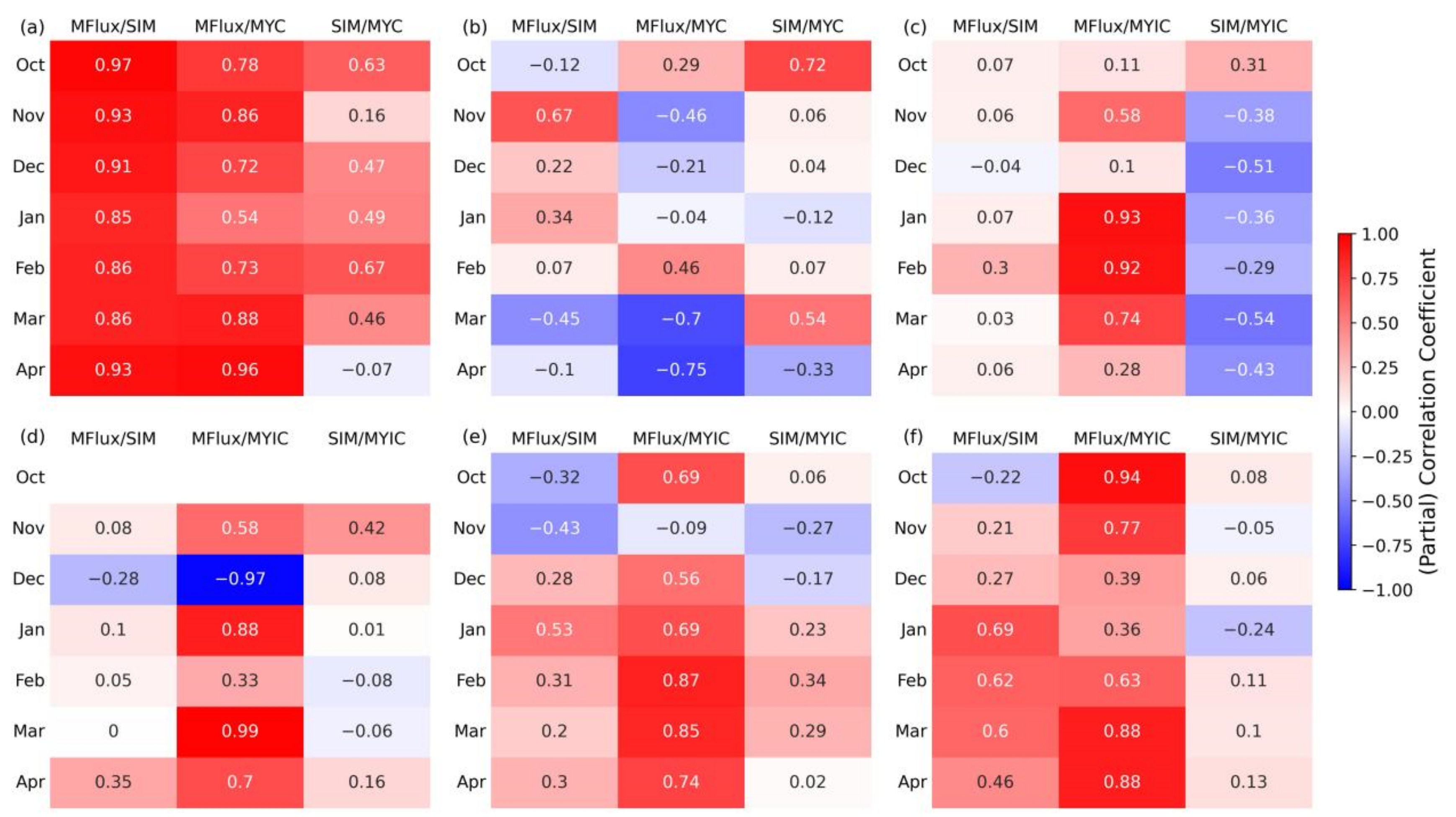
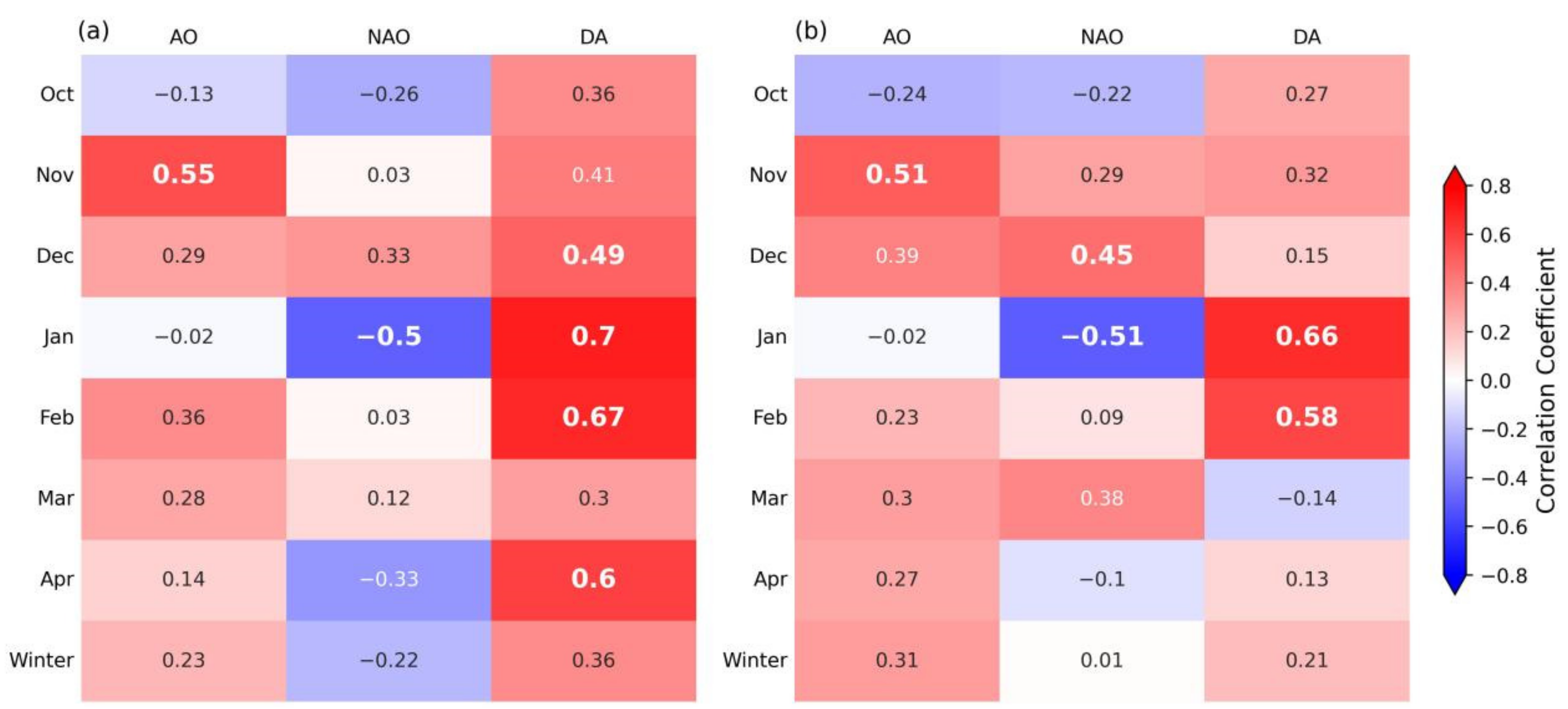
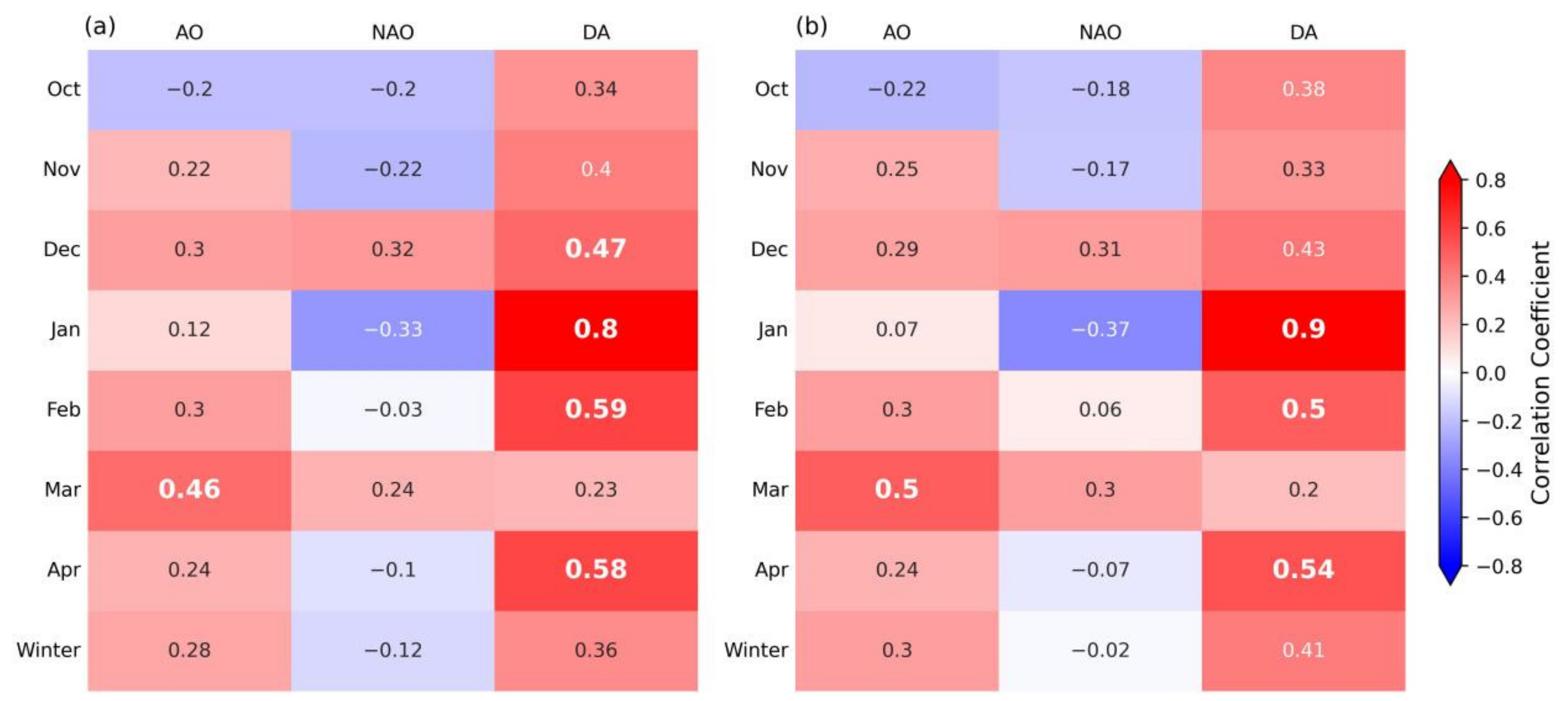
4.3. Connection between Sea Ice Outflow and Varying Atmospheric Indices

In order to investigate the relationships between the ice flux (total sea ice and MYI) and atmospheric circulations, the correlations with three atmospheric indices (AO, NAO, DA) for the wintertime and each separate month (October–April) were examined based on detrended time series. The computed CCs for Fram Strait and the Arctic are presented (total sea ice flux in Figure 8, MYI flux in Figure 9). The other five gates with a very small outflow of sea ice are found with non-significant correlations (not shown).

Overall, DA seems to manifest the strongest correlations with sea ice flux (total sea ice and MYI) in Fram Strait and of the Arctic in most winter months, whereas AO and NAO (especially the latter) demonstrate weaker linkages.

In terms of total sea ice outflow (Figure 8), the correlations between AO and areal flux are positive in general. The strongest correlations appear in November, with a positive CC of 0.55 (p < 0.05) and 0.51 (p < 0.05) for Fram Strait and the Arctic, respectively. In comparison, the correlations between NAO and total sea ice outflow are negative in some months. The strongest linkages occur in January with a negative CC of −0.50 in Fram Strait (Figure 8a) and −0.51 in the Arctic (Figure 8b) at the 95% significant level. For DA, it demonstrates the highest positive correlation among the three atmospheric indices with the total sea ice areal flux. In January, the correlations reach the maximum, with CC of 0.70 (p < 0.01) in Fram Strait and 0.66 (p < 0.01) of the Arctic.

Similarly, the correlations between MYI areal flux and AO/NAO are collectively weaker than those with DA. Correlations between AO and MYI flux are positive in general. The strongest linkages appear in March, with positive CC of 0.46 (p < 0.05) in Fram Strait (Figure 9a) and 0.50 (p < 0.05) of the Arctic (Figure 9b), respectively. The correlations between NAO and MYI flux are negative in most cases and weak generally.

It should be noted that the connections between DA and MYI flux are even stronger than that between DA and total sea ice flux in some months. Particularly, the CCs in January are as high as 0.80 (p < 0.01) and 0.90 (p < 0.01) through Fram Strait and of the Arctic, respectively. This indicates that DA poses a significant impact on modulating the sea ice, especially the MYI outflow. It may be due to the fact that the total sea ice, which contains thinner and more fragile ice such as FYI, could be susceptible to other synoptic and climatic factors. As well, the thicker MYI is mainly affected by the large-scale atmospheric circulations and less sensitive to some instantaneous synoptic conditions.

4.4. The Distinct Role of Arctic Dipole Anomaly

As mentioned in Section 4.3, DA is highly correlated with sea ice flux in January. Such connection is further explored in this section. Figure 10 shows the time series of sea ice flux and DA index in January from 2003 to 2021. It is clear that the DA index is generally consistent with the sea ice areal flux. Sea ice outflow is relatively high when DA is in its positive phase, and vice versa.

This is because when DA is situated in different phases, two opposite SLP anomalies centers are identified in the Arctic Basin, which regulates the variation of sea ice flux through Fram Strait. During the positive phase of DA, the Beaufort Gyre is weakened, favoring sea ice export out of the Arctic Ocean through Fram Strait. In the opposite situation, the strengthened Beaufort Gyre accumulates sea ice and freshwater in the Arctic Basin and reduces the sea ice export.

To investigate and verify the mechanism of atmospheric SLP patterns on the sea ice export through Fram Strait, we obtained the ERA5 SLP anomaly fields of January 2017 (Figure 11a) and 2006 (Figure 11b) when DA is situated in the positive and negative phase, respectively.

As shown in Figure 11, an east-west pattern is found with two centers of action situated in the Barents-Kara Seas and Greenland-Canadian Archipelago sides, which resembles the DA-SLP structure. When DA remains in its positive phase (Figure 11a), the Greenland side shows extensive positive SLP anomalies and the Barents side presents concurrent negative anomalies, which results in a strengthened cross-gate SLP gradient thus facilitating the sea ice export through Fram Strait. While during the negative DA phase (Figure 11b), an opposite pattern is observed, leading to a weaken cross-gate SLP gradient and restricting the sea ice outflow.

The above-mentioned east-west dipole pattern of Greenland-positive/negative and the Barents-negative/positive is associated with the geostrophic northerly/southerly winds through Fram Strait and physically related to the increase/decrease of sea ice outflow [53]. In addition, sea ice drift is determined largely by the wind above and the ocean current below the sea ice [54]. For short timescales and in all seasons, the sea ice motion is mostly wind-driven with more than 70% of the variance explained by geostrophic winds [55]. Thus it is expected to have a certain impact on the sea ice outflow especially when the wind pattern is controlled by a mode such as DA.

Figure 11 also reveals the wind fields of January 2017 and 2006, while Figure 12 depicts the corresponding sea ice motion fields. As can be seen, when DA is in the positive phase, the wind is blowing from the Arctic Ocean to the lower latitudes through Fram Strait (Figure 11a), sea ice drifts following the wind and flows in the same pattern (Figure 12a), which is favorable for sea ice export through Fram Strait. On the contrary, when DA is situated in the negative phase, the wind blows from the lower latitudes towards the Arctic Ocean (Figure 11b) and sea ice drifts northward as well (Figure 12b), under which the sea ice outflow is largely inhibited instead.

5. Discussion

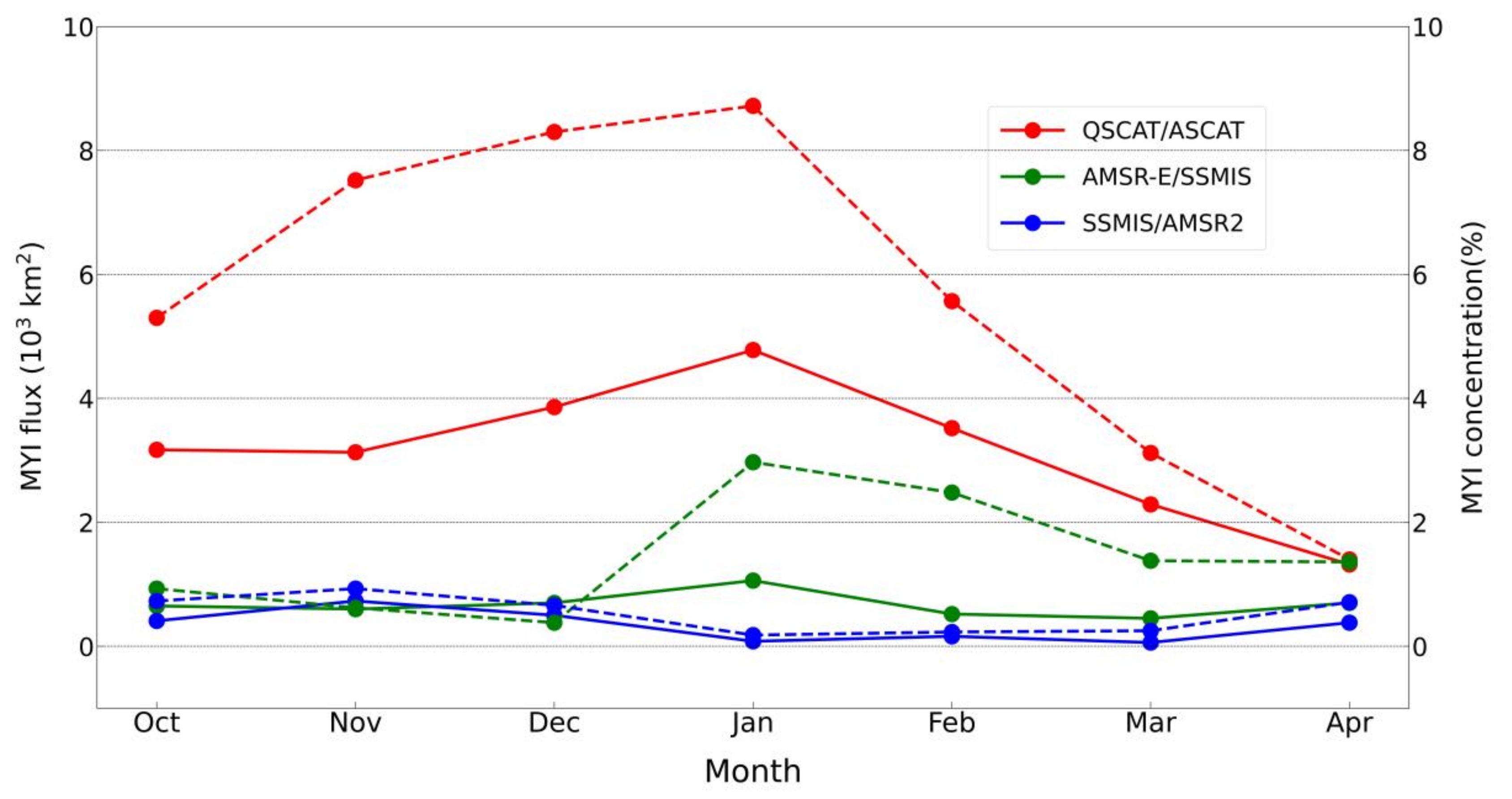
5.1. Consistency of MYI Concentration Data and Its Influence on MYI Flux

For time series analysis, it is crucial to have a consistent dataset. In order to establish a consistent MYI concentration data for the years of 2002–2021, the following three factors have been accounted for in the processing: (1) differences caused by the inconsistent spatial resolution; (2) discrepancies due to the different sets of satellite inputs; (3) differences induced by the thresholds and criteria of the post-processing correction schemes.

To account for the first factor, all the satellite data are resampled into the same grid spacing of 12.5 km, which further ensures the consistent performance of the post-processing correction schemes as long as the thresholds keep the same. For the second factor, the MYI concentration derived from ECICE with the four sets of inputs is normalized for the overlapping periods of each pair (Section 3.3). Monthly differences for the three pairs of datasets are shown in Figure 13. Among them, the largest discrepancy occurs when different scatterometer data are used (QSCAT and ASCAT), with an average of about 3.15 × 10³ km² along all the fluxgates. In comparison, discrepancies induced by the different radiometer data are much smaller, the average of which is only 0.67 × 10³ km² (AMSR-E and SSMIS) and 0.33 × 10³ km² (SSMIS and AMSR2), respectively.

As indicated in Section 4, there is a slight decreasing trend for the wintertime Arctic MYI flux through all gates over the past two decades, with decreasing rate of about −9.2%/decade. Without considering the discrepancies, the declining trend is about −43.7%/decade from 2002 to 2021, which is much stronger than the results after normalization. Similar changes are found for the MYI flux through Fram Strait. The declining trend is −29.2%/decade and −2.9%/decade, respectively, before and after normalization. For the third factor, when applying the correction scheme with sea ice drift to restore the overestimated MYI concentration [48], we adjusted the threshold for defining the MYI domain from 15% to 20% to account for the impact of different spatial resolutions (4.45 km and 12.5 km for the original and new MYI concentration, respectively). Thresholds were determined empirically using SAR images as the verification data.

A recent study presents the MYI flux through Fram Strait [25], where different sets of MYI concentration data are used and the consistency is not considered. It is shown that, the wintertime MYI areal flux declined by 22% from 382.4 × 10³ km² in 2002/2003–2010/2011 to 300.8 × 10³ km² in 2012/2013–2019/2020. In comparison, the MYI flux in our study, which considers the above three factors, only shows a slight decrease of 6% in the corresponding periods (from 342.0 × 10³ km² to 320.2 × 10³ km²). All the above-mentioned factors contribute to the inconsistency of MYI flux time series, which eventually lead to an overall 16% difference in the Fram Strait MYI flux declining rate for the two periods. This indicates that inconsistencies in spatial resolution and data sources have a significant impact on the MYI flux estimates and thus should be considered with caution.

5.2. Variability of MYI Areal Flux, Total Sea Ice Areal and Volume Flux

This section investigates the linkages between MYI areal flux and total sea ice areal as well as volume flux. On one hand, a large part of the Arctic sea ice is MYI, the variability of MYI areal flux is thus usually correlated with the total sea ice areal flux. On the other hand, as a proxy of thick sea ice, the areal flux of MYI indicates the flux of thick sea ice, which could also influence the sea ice volume flux.

As shown in Section 4.1, the inter-annual variability of Arctic MYI areal flux and total sea ice areal flux are quite consistent with each other (CC of 0.67). Both exhibit a slight declining trend in the winters of 2002–2021, with a declining rate of −3.4 × 10³ km²/year (−9.2%/decade) and −7.4 × 10³ km²/year (−9.8%/decade), respectively. Arctic MYI areal flux accounts for about half (49.3%) of the total sea ice areal flux on average with a slight negative trend (−0.4%/decade) in the proportion of the latter over the past two decades, yet its inter-annual variation is quite significant (standard deviation of 7.9%) (Figure 14). As for the sea ice flux through Fram Strait, the inter-annual variability of MYI areal flux is highly correlated with that of the total sea ice outflow (CC up to 0.83). While there is a subtle negative trend in the MYI areal flux with a decreasing rate of −0.9 × 10³ km²/year (−2.9%/decade), the total sea ice areal flux exhibits a slight positive variation trend (1.2 × 10³ km²/year or 2.7%/decade). Similar total sea ice areal flux variabilities through Fram Strait have been found in previous studies [18,33,54]. Winter MYI flux via Fram Strait occupies more than two-thirds (69.6%) of its total sea ice export on average. The ratio of MYI flux to total sea ice flux in Fram Strait exhibits a much more pronounced negative trend (−5.3%/decade) than that of the Arctic (−0.4%/decade) over the past two decades, which indicates an increasing portion of FYI exported through Fram Strait. Additionally, the inter-annual variation of this proportion is comparable to that of the Arctic with a standard deviation of 6.6%.

The long-term decreasing trend in the Arctic total sea ice areal flux for the winters of 2002–2021 is mainly attributed to the significant decline since 2006/2007 (Figure 4a), when the declining rate reaches −20.42 × 10³ km²/year (26.58%/decade). A similar pattern is found in the Arctic MYI areal flux, which exhibits a stronger declining rate (−7.42 × 10³ km²/year or 19.75%/decade) during 2006–2021 than that for 2002–2021 (Figure 4b). Moreover, MYI flux through the four fluxgates other than Fram Strait and North Gate is nearly zero since 2007/2008. With nearly constant MYI flux through North Gate for 2007–2021, the inter-annual trend of Arctic MYI flux keeps in line with that through Fram Strait. During the winters of 2007–2021, the correlation between Arctic MYI flux and ice concentration/motion is 0.89 and 0.50, respectively, with the enhanced influence of MYI concentration and weakened correlation with ice motion than 2002–2021 (CC of 0.57 and 0.41, respectively).

As mentioned above, MYI areal flux through Fram Strait demonstrates a slight decreasing trend over the past two decades (−2.9%/decade). Moreover, the decline of sea ice thickness during 1958–2018 has been shown in a previous study [56], which leads to a significant declining trend (−27%/decade) in the sea ice volume flux via Fram Strait for the period of 1992–2014 [17]. Exceptions are found in the results from the combined model and satellite data [57,58], where no significant long-term trend in total sea ice volume export could be identified for the years of 1979–2012 and 1990–2010, respectively. This is because the increasing total sea ice areal flux is balanced with the reduced sea ice thickness over time, giving no significant variation trend in the volume outflow. Considering the negative trend of MYI flux in the present study, it can be further confirmed that Arctic sea ice is increasingly dominated by thinner and younger FYI instead of MYI. While FYI makes a greater contribution to total sea ice areal and volume flux, a weakened association between MYI flux and sea ice volume flux is manifested.

5.3. Correlation Analysis of Sea Ice Flux and Atmospheric Indices

The correlation between sea ice flux and atmospheric indices has been investigated in various studies yet different conclusions have been drawn [12,19,25,59,60]. Factors that may influence the correlation analysis include: (1) temporal scale, which ranges from the month, season, year to decade; (2) uncertainty of data source, which could lead to large variations in some cases; (3) atmospheric patterns that may not be captured by the indices, however, have large impacts on sea ice flux.

For the first factor, as it is shown in Section 4.3, winter and monthly sea ice areal flux exhibit different correlations with the three atmospheric indices. High correlations occur in certain winter months. For instance, DA demonstrates the strongest correlation with sea ice flux in January. Delay effects may also play a non-negligible role in the correlations. Wang et al. [25] explored the correlations between monthly MYI areal export and the three atmospheric indices with lags from 0 to 7 months. For DA, the correlation with sea ice flux is greatest when the lag is 0 months. Since the correlation between sea ice flux and atmospheric circulation varies with month, results may differ when the analysis is performed for different spans of months. The correlation between winter (October–April) total sea ice areal export and AO index is 0.22 (Figure 8a) in this study, whereas it is about 0.53 for the winter (December–March) in [19]. Discrepancies are even more pronounced for winter and annual flux analyses. Winter NAO exhibits a weak linkage with the winter total sea ice flux for 2002–2021 (CC of −0.23, shown in Figure 8a), while Dickson et al. [59] reported that the inter-annual variations of the winter NAO index explain about 60% of the variance (i.e., R² = 0.6) in the annual total sea ice flux since 1976. It can be seen that results based on different temporal scales may differ from each other.

For the second factor, as mentioned in Section 5.1, bias may exist in the sea ice flux due to the application of different data sources and techniques. This may further impact its variability and correlation with atmospheric indices. Sea ice areal export could be estimated based on an empirical relationship with the SLP gradients across Fram Strait [54]. Results indicate that there is a clear increasing trend in the sea ice flux from 1957–2010. In comparison, the sea ice areal export estimated from a combination of satellite radar images and station observations of surface pressure exhibit no long-term trend from 1935–2014 [61]. Such discrepancies exist in the sea ice flux, thus the correlation between the sea ice outflow and atmospheric indices could be varying.

With respect to the third factor, the atmospheric indices can merely characterize the corresponding circulation patterns in general. Despite the same atmospheric index, the center of the SLP anomaly may exhibit inconsistent mode (Figure 15). This results in different wind field patterns thus leading to different sea ice outflow and correlations. As it is found in [60], the wintertime correlation between NAO and sea ice export through Fram Strait varies from 0.1 (1958–1977) to about 0.7 (1978–1997), which is attributed to the anomalous meridional wind components associated with the more easterly position of NAO center.

All the above three factors contribute to the varying correlations between sea ice flux and atmospheric indices. They should be treated with caution for further investigation of the connection between atmospheric circulations and sea ice flux.

6. Conclusions

This study presents MYI and total sea ice areal flux through six Arctic gateways over the winters (October–April) of 2002–2021 estimated with daily gridded sea ice motion and MYI/total sea ice concentration fields. Systematic biases caused by different data sources were examined for the estimate of MYI areal flux. On this basis, inter-annual and monthly variability of the sea ice flux were analyzed. The contribution of sea ice motion and sea ice concentration to the areal flux was investigated, and the connections between sea ice flux and three climate indices (AO, NAO, DA) were explored. Furthermore, linkages between the MYI areal flux and total sea ice areal/volume flux, as well as the possible influencing factors on the correlation between sea ice flux and atmospheric indices were discussed.

It is found that, discrepancies in the Arctic MYI areal flux calculated from the MYI concentration estimates from the different microwave observations can be significant and should be taken into account in the inter-annual analysis. The largest discrepancy of the Arctic MYI areal flux occurs when different scatterometer data are used in the winters of 2007–2009, with the average bias of 111.60 × 10³ km². Such discrepancy highly influences the estimated inter-annual trend of the MYI areal flux. Without accounting for the inconsistencies, the Arctic MYI areal flux exhibits a declining trend of −43.7%/decade from 2002 to 2021, while the declining rate is only −9.2%/decade when inconsistencies are removed by the normalization procedure.

There are slight decreasing trends in the Arctic total sea ice and MYI areal flux over the past two decades, mainly due to the decrease in sea ice concentration. The average wintertime total sea ice areal flux is 468.30 × 10³ km² and 759.02 × 10³ km² through Fram Strait and all the Arctic fluxgates, respectively, whereas the MYI areal flux is 325.92 × 10³ km² and 373.72 × 10³ km², respectively. Total sea ice flux via Fram Strait occupies ~62% of the Arctic flux, while MYI flux in Fram Strait accounts for a larger proportion of ~87% of the Arctic in winter. Since the areal flux of thick MYI takes up a large proportion of the total sea ice areal flux (69.6% through Fram Strait and 49.3% of the Arctic), MYI areal flux may characterize total sea ice areal and volume flux to some extent.

In regard to the monthly variability of sea ice outflow (total sea ice and MYI), it is found that sea ice flux through Fram Strait and of the Arctic demonstrate mild increasing trends with fluctuations from October to March, yet a significant decline in April. In general, there are slight increasing trends in the total sea ice flux through Fram Strait and of the Arctic from October to April, yet no obvious monthly trends are identified in the MYI flux.

For total sea ice, the ice motion rather than ice concentration can better explain the variability of the areal flux in the three main gateways of ice flux (i.e., Fram Strait, FJ–SZ and North Gate). While for MYI, the contributions of sea ice motion and MYI concentration to the MYI areal flux are comparatively large in Fram Strait, yet the MYI concentration plays a more dominant role in North Gate. MYI flux through the other four gates is much smaller and does not exhibit clear patterns of the dominant factor (ice motion/concentration).

Correlations between the monthly sea ice flux and NAO are relatively weak (even weaker with AO), while that with DA is much stronger. CC between the Arctic MYI flux and DA reaches 0.90 (p < 0.01) in January. To further investigate the relationship between DA and sea ice flux through Fram Strait, SLP anomaly, 10 m wind fields, and sea ice motion patterns were analyzed for specific situations. When DA is situated in the positive phase, a strengthened cross-strait SLP gradient together with the northerly wind and sea ice drift is observed, contributing to an enhanced sea ice export through Fram Strait. In contrast, when DA is in the negative phase, a weakened cross-strait SLP gradient together with the southerly wind and sea ice drift is expected, which inhibits the sea ice outflow. While it should be mentioned that, sea ice flux estimated during different periods based on multi-source data and methods may demonstrate different correlations with the atmospheric indices. Additionally, atmospheric circulation patterns may not be fully captured by the atmospheric indices, the same value of atmospheric indices could imply different atmospheric situations and thus have different influences on sea ice flux.

In this paper, we focused on the connection between DA and sea ice export through Fram Strait from the perspective of SLP, wind fields, and ice motion patterns. Nevertheless, this may not be explanatory for other fluxgates. For instance, sea ice outflow through North Gate and Lanscater Sound may be affected by the formation or absence of ice arches [23,62,63]. Mechanisms of such deserve further exploration.

References

1. Meier, W.N.; Hovelsrud, G.K.; Van Oort, B.E.; Key, J.R.; Kovacs, K.M.; Michel, C.; Haas, C.; Granskog, M.A.; Gerland, S.; Perovich, D.K. Arctic sea ice in transformation: A review of recent observed changes and impacts on biology and human activity. Rev. Geophys. 2014, 52, 185–217. [Google Scholar] [CrossRef]
2. Johannessen, O.M.; Bengtsson, L.; Miles, M.W.; Kuzmina, S.I.; Semenov, V.A.; Alekseev, G.V.; Nagurnyi, A.P.; Zakharov, V.F.; Bobylev, L.P.; Pettersson, L.H. Arctic climate change: Observed and modelled temperature and sea-ice variability. Tellus A Dyn. Meteorol. Oceanogr. 2004, 56, 328–341. [Google Scholar] [CrossRef]
3. Stroeve, J.; Notz, D. Changing state of Arctic sea ice across all seasons. Environ. Res. Lett. 2018, 13, 103001. [Google Scholar] [CrossRef]
4. Thackeray, C.W.; Hall, A. An emergent constraint on future Arctic sea-ice albedo feedback. Nat. Clim. Chang. 2019, 9, 972–978. [Google Scholar] [CrossRef]
5. Donohoe, A.; Blanchard-Wrigglesworth, E.; Schweiger, A.; Rasch, P.J. The effect of atmospheric transmissivity on model and observational estimates of the sea ice albedo feedback. J. Clim. 2020, 33, 5743–5765. [Google Scholar] [CrossRef] [Green Version]
6. Cavalieri, D.J.; Parkinson, C.L. Arctic sea ice variability and trends, 1979–2010. Cryosphere 2012, 6, 881–889. [Google Scholar] [CrossRef] [Green Version]
7. Comiso, J.C.; Parkinson, C.L.; Gersten, R.; Stock, L. Accelerated decline in the Arctic sea ice cover. Geophys. Res. Lett. 2008, 35, L01703. [Google Scholar] [CrossRef] [Green Version]
8. Comiso, J.C. Large decadal decline of the Arctic multiyear ice cover. J. Clim. 2012, 25, 1176–1193. [Google Scholar] [CrossRef]
9. Stroeve, J.; Holland, M.M.; Meier, W.; Scambos, T.; Serreze, M. Arctic sea ice decline: Faster than forecast. Geophys. Res. Lett. 2007, 34. [Google Scholar] [CrossRef]
10. Kwok, R. Near zero replenishment of the Arctic multiyear sea ice cover at the end of 2005 summer. Geophys. Res. Lett. 2007, 34, L05501. [Google Scholar] [CrossRef]
11. Kwok, R.; Untersteiner, N. The thinning of Arctic sea ice. Phys. Today 2011, 64, 36–41. [Google Scholar] [CrossRef] [Green Version]
12. Ricker, R.; Girard-Ardhuin, F.; Krumpen, T.; Lique, C. Satellite-derived sea ice export and its impact on Arctic ice mass balance. Cryosphere 2018, 12, 3017–3032. [Google Scholar] [CrossRef] [Green Version]
13. Bi, H.; Wang, Y.; Zhang, W.; Zhang, Z.; Liang, Y.; Zhang, Y.; Hu, W.; Fu, M.; Huang, H. Recent satellite-derived sea ice volume flux through the Fram Strait: 2011–2015. Acta Oceanol. Sin. 2018, 37, 107–115. [Google Scholar] [CrossRef]
14. Semmling, A.M.; Rösel, A.; Divine, D.V.; Gerland, S.; Stienne, G.; Reboul, S.; Ludwig, M.; Wickert, J.; Schuh, H. Sea-ice concentration derived from GNSS reflection measurements in Fram Strait. IEEE Trans. Geosci. Remote Sens. 2019, 57, 10350–10361. [Google Scholar] [CrossRef]
15. Serreze, M.C.; Barrett, A.P.; Slater, A.G.; Woodgate, R.A.; Aagaard, K.; Lammers, R.B.; Steele, M.; Moritz, R.; Meredith, M.; Lee, C.M. The large-scale freshwater cycle of the Arctic. J. Geophys. Res. Ocean. 2006, 111. [Google Scholar] [CrossRef] [Green Version]
16. Spreen, G.; Kern, S.; Stammer, D.; Hansen, E. Fram Strait sea ice volume export estimated between 2003 and 2008 from satellite data. Geophys. Res. Lett. 2009, 36, L19502. [Google Scholar] [CrossRef]
17. Spreen, G.; de Steur, L.; Divine, D.; Gerland, S.; Hansen, E.; Kwok, R. Arctic sea ice volume export through Fram Strait from 1992 to 2014. J. Geophys. Res. Ocean. 2020, 125, e2019JC016039. [Google Scholar] [CrossRef]
18. Kwok, R.; Cunningham, G.; Pang, S. Fram Strait sea ice outflow. J. Geophys. Res. Ocean. 2004, 109. [Google Scholar] [CrossRef]
19. Kwok, R. Outflow of Arctic Ocean sea ice into the Greenland and Barents Seas: 1979–2007. J. Clim. 2009, 22, 2438–2457. [Google Scholar] [CrossRef] [Green Version]
20. Kwok, R.; Toudal Pedersen, L.; Gudmandsen, P.; Pang, S. Large sea ice outflow into the Nares Strait in 2007. J. Geophys. Res. Lett. 2010, 37. [Google Scholar] [CrossRef] [Green Version]
21. Krumpen, T.; Janout, M.; Hodges, K.; Gerdes, R.; Girard-Ardhuin, F.; Hölemann, J.A.; Willmes, S. Variability and trends in Laptev Sea ice outflow between 1992–2011. Cryosphere 2013, 7, 349–363. [Google Scholar] [CrossRef] [Green Version]
22. Agnew, T.; Lambe, A.; Long, D. Estimating sea ice area flux across the Canadian Arctic Archipelago using enhanced AMSR-E. J. Geophys. Res. Ocean. 2008, 113. [Google Scholar] [CrossRef] [Green Version]
23. Bi, H.; Zhang, Z.; Wang, Y.; Xu, X.; Liang, Y.; Huang, J.; Liu, Y.; Fu, M. Baffin Bay sea ice inflow and outflow: 1978–1979 to 2016–2017. Cryosphere 2019, 13, 1025–1042. [Google Scholar] [CrossRef] [Green Version]
24. Belmonte Rivas, M.; Otosaka, I.; Stoffelen, A.; Verhoef, A. A scatterometer record of sea ice extents and backscatter: 1992–2016. Cryosphere 2018, 12, 2941–2953. [Google Scholar] [CrossRef] [Green Version]
25. Wang, Y.; Bi, H.; Liang, Y. A Satellite-Observed Substantial Decrease in Multiyear Ice Area Export through the Fram Strait over the Last Decade. Remote Sens. 2022, 14, 2562. [Google Scholar] [CrossRef]
26. Jahn, A.; Tremblay, B.; Mysak, L.A.; Newton, R. Effect of the large-scale atmospheric circulation on the variability of the Arctic Ocean freshwater export. Clim. Dyn. 2010, 34, 201–222. [Google Scholar] [CrossRef]
27. Mikolajewicz, U.; Sein, D.V.; Jacob, D.; Königk, T.; Podzun, R.; Semmler, T. Simulating Arctic sea ice variability with a coupled regional atmosphere-ocean-sea ice model. Meteorol. Z. 2005, 14, 793–800. [Google Scholar] [CrossRef] [Green Version]
28. Li, M.; Ke, C.; Cheng, B.; Shen, X.; He, Y.; Sha, D. The Roles of Sea Ice Export, Atmospheric and Oceanic Factors in the Seasonal and Regional Variability of Arctic Sea Ice during 1979–2020. Remote Sens. 2022, 14, 904. [Google Scholar] [CrossRef]
29. Wettstein, J.J.; Deser, C. Internal variability in projections of twenty-first-century Arctic sea ice loss: Role of the large-scale atmospheric circulation. J. Clim. 2014, 27, 527–550. [Google Scholar] [CrossRef] [Green Version]
30. Thompson, D.W.; Wallace, J.M. The Arctic Oscillation signature in the wintertime geopotential height and temperature fields. Geophys. Res. Lett. 1998, 25, 1297–1300. [Google Scholar] [CrossRef] [Green Version]
31. Hurrell, J.W. Decadal trends in the North Atlantic Oscillation: Regional temperatures and precipitation. Science 1995, 269, 676–679. [Google Scholar] [CrossRef] [PubMed] [Green Version]
32. Wu, B.; Wang, J.; Walsh, J.E. Dipole anomaly in the winter Arctic atmosphere and its association with sea ice motion. J. Clim. 2006, 19, 210–225. [Google Scholar] [CrossRef]
33. Kwok, R.; Rothrock, D.A. Variability of Fram Strait ice flux and North Atlantic oscillation. J. Geophys. Res. Ocean. 1999, 104, 5177–5189. [Google Scholar] [CrossRef] [Green Version]
34. Kwok, R.; Spreen, G.; Pang, S. Arctic sea ice circulation and drift speed: Decadal trends and ocean currents. J. Geophys. Res. Ocean. 2013, 118, 2408–2425. [Google Scholar] [CrossRef]
35. Jung, T.; Hilmer, M. The link between the North Atlantic Oscillation and Arctic sea ice export through Fram Strait. J. Clim. 2001, 14, 3932–3943. [Google Scholar] [CrossRef] [Green Version]
36. Rigor, I.G.; Wallace, J.M.; Colony, R.L. Response of sea ice to the Arctic Oscillation. J. Clim. 2002, 15, 2648–2663. [Google Scholar] [CrossRef] [Green Version]
37. Wei, J.; Zhang, X.; Wang, Z. Reexamination of Fram Strait sea ice export and its role in recently accelerated Arctic sea ice retreat. Clim. Dyn. 2019, 53, 1823–1841. [Google Scholar] [CrossRef] [Green Version]
38. Lei, R.; Gui, D.; Hutchings, J.K.; Wang, J.; Pang, X. Backward and forward drift trajectories of sea ice in the northwestern Arctic Ocean in response to changing atmospheric circulation. Int. J. Climatol. 2019, 39, 4372–4391. [Google Scholar] [CrossRef] [Green Version]
39. Zhang, F.; Pang, X.; Lei, R.; Zhai, M.; Zhao, X.; Cai, Q. Arctic sea ice motion change and response to atmospheric forcing between 1979 and 2019. Int. J. Climatol. 2022, 42, 1854–1876. [Google Scholar] [CrossRef]
40. Shokr, M.; Lambe, A.; Agnew, T. A new algorithm (ECICE) to estimate ice concentration from remote sensing observations: An application to 85-GHz passive microwave data. IEEE Trans. Geosci. Remote Sens. 2008, 46, 4104–4121. [Google Scholar] [CrossRef]
41. Steffen, K.; Abdalati, W.; Stroeve, J. Climate sensitivity studies of the Greenland ice sheet using satellite AVHRR, SMMR, SSM/I and in situ data. Meteorol. Atmos. Phys. 1993, 51, 239–258. [Google Scholar] [CrossRef] [Green Version]
42. Tschudi, M.A.; Meier, W.N.; Stewart, J.S. An enhancement to sea ice motion and age products at the National Snow and Ice Data Center (NSIDC). Cryosphere 2020, 14, 1519–1536. [Google Scholar] [CrossRef]
43. Hersbach, H. The ERA5 Atmospheric Reanalysis. In Proceedings of the AGU Fall Meeting Abstracts, San Francisco, CA, USA, 12–16 December 2016; p. NG33D-01. [Google Scholar]
44. Hersbach, H.; Bell, B.; Berrisford, P.; Hirahara, S.; Horányi, A.; Muñoz-Sabater, J.; Nicolas, J.; Peubey, C.; Radu, R.; Schepers, D. The ERA5 global reanalysis. Q. J. R. Meteorol. Soc. 2020, 146, 1999–2049. [Google Scholar] [CrossRef]
45. Bi, H.; Sun, K.; Zhou, X.; Huang, H.; Xu, X. Arctic Sea ice area export through the Fram Strait estimated from satellite-based data: 1988–2012. IEEE J. Sel. Top. Appl. Earth Obs. Remote Sens. 2016, 9, 3144–3157. [Google Scholar] [CrossRef]
46. Wang, J.; Zhang, J.; Watanabe, E.; Ikeda, M.; Mizobata, K.; Walsh, J.E.; Bai, X.; Wu, B. Is the Dipole Anomaly a major driver to record lows in Arctic summer sea ice extent? Geophys. Res. Lett. 2009, 36. [Google Scholar] [CrossRef] [Green Version]
47. Shokr, M.; Agnew, T.A. Validation and potential applications of Environment Canada Ice Concentration Extractor (ECICE) algorithm to Arctic ice by combining AMSR-E and QuikSCAT observations. Remote Sens. Environ. 2013, 128, 315–332. [Google Scholar] [CrossRef]
48. Ye, Y.; Shokr, M.; Heygster, G.; Spreen, G. Improving multiyear sea ice concentration estimates with sea ice drift. Remote Sens. 2016, 8, 397. [Google Scholar] [CrossRef] [Green Version]
49. Ye, Y.; Shokr, M.; Aaboe, S.; Aldenhoff, W.; Eriksson, L.E.; Heygster, G.; Melsheimer, C.; Girard-Ardhuin, F. Inter-comparison and evaluation of sea ice type concentration algorithms. Cryosphere Discuss. 2019, 1–30. [Google Scholar] [CrossRef] [Green Version]
50. Hao, G.; Su, J. A study of multiyear ice concentration retrieval algorithms using AMSR-E data. Acta Oceanol. Sin. 2015, 34, 102–109. [Google Scholar] [CrossRef]
51. Sinha, N.K.; Shokr, M. Sea Ice: Physics and Remote Sensing; John Wiley & Sons: Hoboken, NJ, USA, 2015. [Google Scholar]
52. Ye, Y.; Heygster, G.; Shokr, M. Improving multiyear ice concentration estimates with reanalysis air temperatures. IEEE Trans. Geosci. Remote Sens. 2015, 54, 2602–2614. [Google Scholar] [CrossRef]
53. Tsukernik, M.; Deser, C.; Alexander, M.; Tomas, R. Atmospheric forcing of Fram Strait sea ice export: A closer look. Clim. Dyn. 2010, 35, 1349–1360. [Google Scholar] [CrossRef] [Green Version]
54. Smedsrud, L.H.; Sirevaag, A.; Kloster, K.; Sorteberg, A.; Sandven, S. Recent wind driven high sea ice area export in the Fram Strait contributes to Arctic sea ice decline. Cryosphere 2011, 5, 821–829. [Google Scholar] [CrossRef] [Green Version]
55. Thorndike, A.; Colony, R. Sea ice motion in response to geostrophic winds. J. Geophys. Res. Ocean. 1982, 87, 5845–5852. [Google Scholar] [CrossRef]
56. Kwok, R. Arctic sea ice thickness, volume, and multiyear ice coverage: Losses and coupled variability (1958–2018). Environ. Res. Lett. 2018, 13, 105005. [Google Scholar] [CrossRef]
57. Zhang, Z.; Bi, H.; Sun, K.; Huang, H.; Liu, Y.; Yan, L. Arctic sea ice volume export through the Fram Strait from combined satellite and model data: 1979–2012. Acta Oceanol. Sin. 2017, 36, 44–55. [Google Scholar] [CrossRef]
58. Zamani, B.; Krumpen, T.; Smedsrud, L.H.; Gerdes, R. Fram Strait sea ice export affected by thinning: Comparing high-resolution simulations and observations. Clim. Dyn. 2019, 53, 3257–3270. [Google Scholar] [CrossRef]
59. Dickson, R.; Osborn, T.; Hurrell, J.; Meincke, J.; Blindheim, J.; Adlandsvik, B.; Vinje, T.; Alekseev, G.; Maslowski, W. The Arctic ocean response to the North Atlantic oscillation. J. Clim. 2000, 13, 2671–2696. [Google Scholar] [CrossRef]
60. Hilmer, M.; Jung, T. Evidence for a recent change in the link between the North Atlantic Oscillation and Arctic sea ice export. Geophys. Res. Lett. 2000, 27, 989–992. [Google Scholar] [CrossRef] [Green Version]
61. Smedsrud, L.H.; Halvorsen, M.H.; Stroeve, J.C.; Zhang, R.; Kloster, K. Fram Strait sea ice export variability and September Arctic sea ice extent over the last 80 years. Cryosphere 2017, 11, 65–79. [Google Scholar] [CrossRef] [Green Version]
62. Kwok, R. Baffin Bay ice drift and export: 2002–2007. Geophys. Res. Lett. 2007, 34. [Google Scholar] [CrossRef] [Green Version]
63. Moore, G.W.K.; Howell, S.E.L.; Brady, M.; Xu, X.; McNeil, K. Anomalous collapses of Nares Strait ice arches leads to enhanced export of Arctic sea ice. Nat. Commun. 2021, 12, 1. [Google Scholar] [CrossRef] [PubMed]
Figure 1. Locations of the six gates for the sea ice outflow estimation.
Remotesensing 14 03742 g001
Figure 2. Flowchart of the areal flux calculation.
Remotesensing 14 03742 g002
Figure 3. Wintertime Arctic MYI areal flux calculated from different data sources.
Remotesensing 14 03742 g003
Figure 4. Winter areal flux of (a) total sea ice and (b) MYI for each fluxgate. Red dotted lines with rectangle and triangle markers represent the mean sea ice concentration and motion of the Arctic, respectively.
Remotesensing 14 03742 g004
Figure 5. The monthly areal flux of (a) total sea ice and (b) MYI for each fluxgate. Red dotted lines with rectangle and triangle markers represent the mean sea ice concentration and motion of the Arctic, respectively.
Remotesensing 14 03742 g005
Figure 6. Partial CCs of total sea ice areal flux (TFlux) with sea ice motion (SIM) and total sea ice concentration (TSIC) as well as the CC between SIM and TSIC in (a) Fram Strait, (b) S–FJ, (c) FJ–SZ, (d) Bering Strait, (e) Lancaster Sound and (f) North Gate.
Remotesensing 14 03742 g006
Figure 7. Partial CCs of MYI areal flux (MFlux) with sea ice motion (SIM) and MYI concentration (MYIC) as well as the CC between SIM and MYIC in (a) Fram Strait, (b) S–FJ, (c) FJ–SZ, (d) Bering Strait, (e) Lanscater Sound and (f) North Gate.
Remotesensing 14 03742 g007
Figure 8. CCs between atmospheric indices and total sea ice areal flux through Fram Strait (a) and of the Arctic (b).
Remotesensing 14 03742 g008
Figure 9. CCs between atmospheric indices and MYI areal flux through Fram Strait (a) and of the Arctic (b).
Remotesensing 14 03742 g009
Figure 10. Inter-annual variability of sea ice areal flux and DA index in January.
Remotesensing 14 03742 g010
Figure 11. ERA5 SLP anomaly and 10 m wind fields of (a) 2017 January (positive DA) and (b) 2006 January (negative DA).
Remotesensing 14 03742 g011
Figure 12. Monthly sea ice motion of (a) 2017 January (positive DA) and (b) 2006 January (negative DA).
Remotesensing 14 03742 g012
Figure 13. Monthly mean differences in MYI areal flux (solid lines) and MYI concentration (dash lines) through all gates caused by different data sources. QSCAT/ASCAT represents the deviation between the two scatterometers, and so on.
Remotesensing 14 03742 g013
Figure 14. The ratio of winter MYI areal flux to the total sea ice areal flux through Fram strait and all the gates of Arctic.
Remotesensing 14 03742 g014
Figure 15. ERA5 SLP anomaly of (a) 2005 January and (b) 2016 January, with the same value of DA index (DA = −0.14).
Remotesensing 14 03742 g015