
Changes in Glaciers and Glacial Lakes in the Bosula Mountain Range, Southeast Tibet, over the past Two Decades


Abstract
:1. Introduction
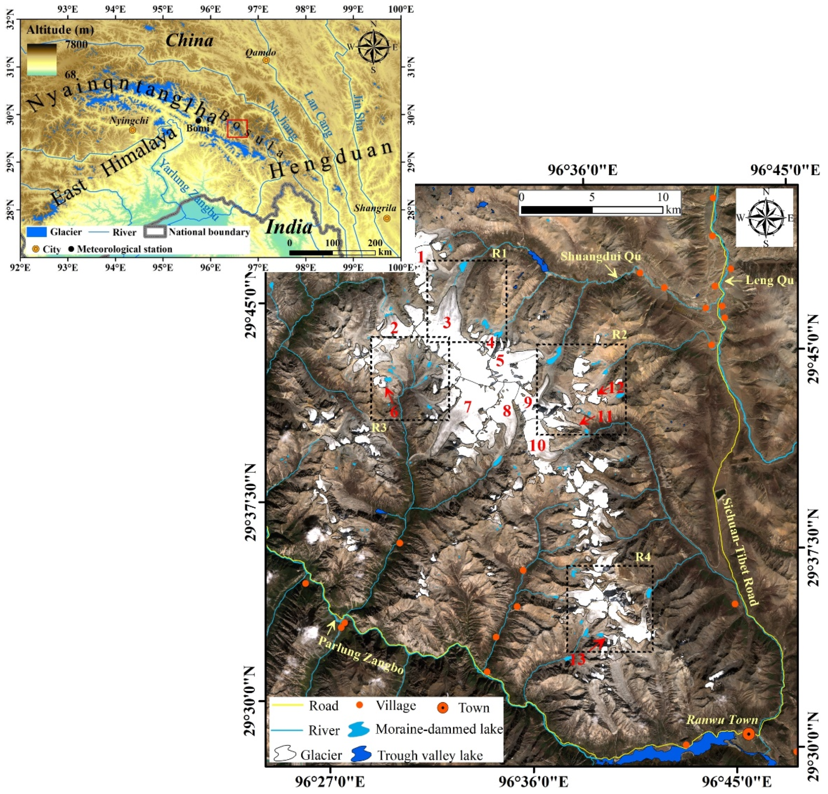
2. Study Area
3. Datasets
3.1. Optical Images
3.2. SAR Images

| Image | Date | Resolution | Product ID | Usage |
|---|---|---|---|---|
| Landsat-5/TM | 27 August 1989 | 30 m | LT51340391989239BJC00 | Glacial lake change interpretation |
| 04 September 1992 | LT51340391992248BJC00 | |||
| 09 October 1993 | LT51340391993282BJC01 | |||
| 12 May 1995 | LT51340391995224BJC00 | |||
| 12 July 2007 | LT51340392007193BJC00 | |||
| 12 June 2008 | LT51340392008164BKT00 | |||
| Landsat-7/ETM | 16 July 2000 | 15 m | LE71340392000198BJC01 | Glacier/glacial lake outline delineation |
| 03 July 2001 | LE71340392001184SGS00 | |||
| Landsat-8/OLI | 13 August 2013 | 15 m | LC81340392013225LGN02 | Glacier/glacial lake outline delineation |
| 22 December 2014 | LC81340392014356LGN01 | Glacier flow velocity estimation | ||
| 24 February 2015 | LC81340392015055LGN01 | |||
| Sentinel-2 | 12 October 2021 | 10 m | S2A_MSIL1C_20211012T040721_N0301_R047_T47RKN_20211012T063225 | Glacier/glacial lake outline delineation |
| 13 November 2015 | S2A_MSIL1C_20151113T041012_N0204_R047_T47RKN_20151113T041259 | Glacier flow velocity estimation | ||
| 23 December 2015 | S2A_MSIL1C_20151223T041202_N0201_R047_T47RKN_20151223T041511 | |||
| 07 December 2016 | S2A_MSIL1C_20161207T041142_N0204_R047_T47RKN_20161207T041633 | |||
| 25 February 2017 | S2A_MSIL1C_20170225T040721_N0204_R047_T47RKN_20170225T041209 | |||
| 02 December 2017 | S2A_MSIL1C_20171202T041131_N0206_R047_T47RKN_20171202T074539 | |||
| 31 January 2018 | S2A_MSIL1C_20180131T041011_N0206_R047_T47RKN_20180131T074139 | |||
| 27 November 2018 | S2A_MSIL1C_20181127T041111_N0207_R047_T47RKN_20181127T065815 | |||
| 16 January 2019 | S2A_MSIL1C_20190116T041121_N0207_R047_T47RKN_20190116T071601 | |||
| 02 November 2019 | S2A_MSIL1C_20191102T040921_N0208_R047_T47RKN_20191102T070601 | |||
| 12 December 2019 | S2A_MSIL1C_20191212T041141_N0208_R047_T47RKN_20191212T070015 | |||
| 16 November 2020 | S2A_MSIL1C_20201116T041041_N0209_R047_T47RKN_20201116T062106 | |||
| 15 January 2021 | S2A_MSIL1C_20210115T041121_N0209_R047_T47RKN_20210115T061909 | |||
| 11 November 2021 | S2A_MSIL1C_20211111T041011_N0301_R047_T47RKN_20211111T051112 | |||
| 09 February 2022 | S2A_MSIL1C_20220209T040921_N0400_R047_T47RKN_20220209T060252 | |||
| TanDEM-X/CoSSC | 17 March 2012 | 1.9 × 2.0 m * | TDM-CoSSC-DEM:/dims_op_pl_dfd_XXXXB00000000293549951504 | DEM extraction |
| 06 December 2015 | 1.9 × 2.0 m * | TDM-CoSSC-Experimental:/dims_op_pl_dfd_XXXXB00000000406913473572 | ||
| 17 December 2019 | 2.4 × 2.0 m * | TDM-CoSSC-DEM:/dims_op_pl_dfd_XXXXB00000000581163692072 |
3.3. NASADEM
3.4. Meteorological Data
4. Methods
4.1. Estimation of Glacier Area and Glacial Lake Area
4.2. Estimation of Change in Glacier Surface Elevation
4.3. Estimation of Glacier Flow Velocity
4.4. Uncertainty Analysis
5. Results
5.1. Changes in Glacier Area and Glacial Lake Area

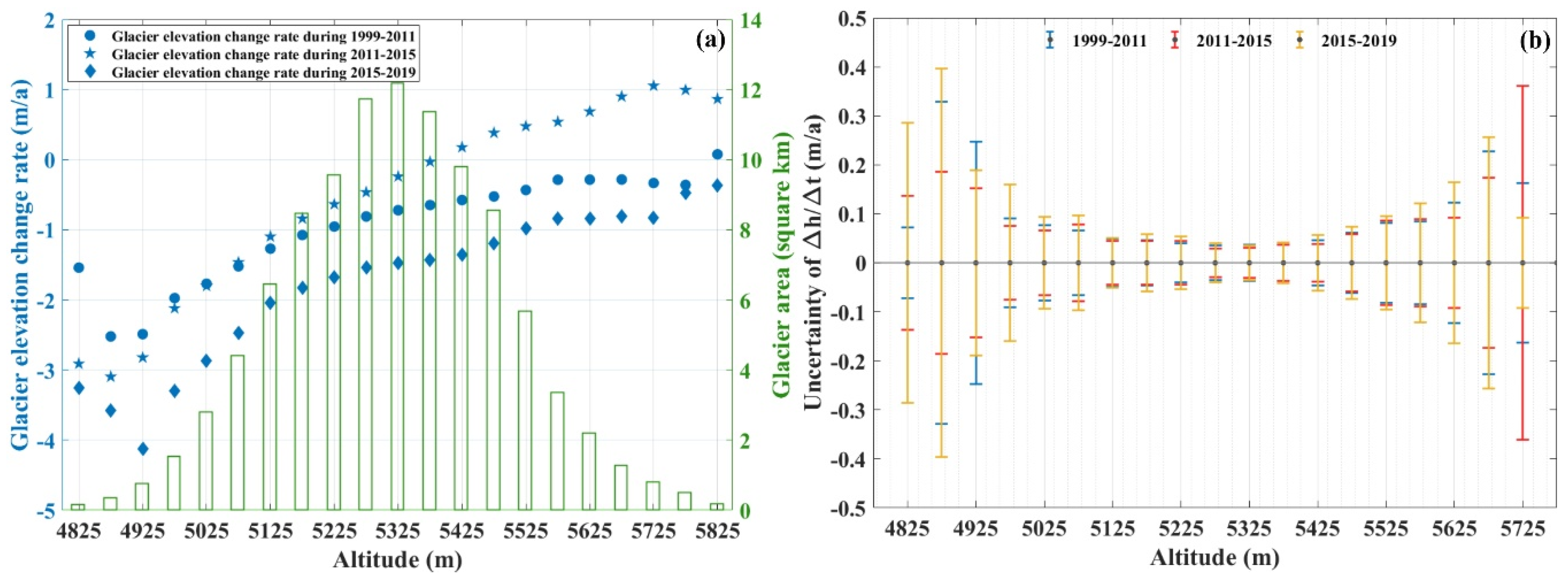
5.2. Change in Glacier Surface Elevation
5.3. Changes in Glacier Flow Velocity
6. Discussion
6.1. Characteristics of Glacier Changes
6.2. Factors of Glacier Change
6.3. Potential Impacts of Glacier Changes on Mountain Hazards
7. Conclusions
Author Contributions
Funding
Acknowledgments
Conflicts of Interest
References
- Wang, W.; Yao, T.; Yang, X. Variations of glacial lakes and glaciers in the Boshula mountain range, southeast Tibet, from the 1970s to 2009. Ann. Glaciol. 2011, 52, 9–17. [Google Scholar] [CrossRef] [Green Version]
- Bazai, N.A.; Cui, P.; Carling, P.A.; Wang, H.; Hassan, J.; Liu, D.; Zhang, G.; Jin, W. Increasing glacial lake outburst flood hazard in response to surge glaciers in the Karakoram. Earth Sci. Rev. 2021, 212, 103432. [Google Scholar] [CrossRef]
- Kamb, B.; Raymond, C.; Harrison, W.; Engelhardt, H.; Echelmeyer, K.; Humphrey, N.; Brugman, M.; Pfeffer, T. Glacier surge mechanism: 1982-1983 surge of Variegated Glacier, Alaska. Science 1985, 227, 469–479. [Google Scholar] [CrossRef] [Green Version]
- Fowler, A. A theory of glacier surges. J. Geophys. Res. Solid Earth 1987, 92, 9111–9120. [Google Scholar] [CrossRef]
- Su, Z.; Shi, Y. Response of monsoonal temperate glaciers to global warming since the Little Ice Age. Quat. Int. 2002, 97, 123–131. [Google Scholar] [CrossRef]
- Hambrey, M.J.; Alean, J.; Alean, J.; Alean, J. Glaciers; Cambridge University Press: Cambridge, UK, 2004; Volume 376. [Google Scholar]
- Kääb, A.; Jacquemart, M.; Gilbert, A.; Leinss, S.; Girod, L.; Huggel, C.; Falaschi, D.; Ugalde, F.; Petrakov, D.; Chernomorets, S. Sudden large-volume detachments of low-angle mountain glaciers–more frequent than thought? Cryosphere 2021, 15, 1751–1785. [Google Scholar] [CrossRef]
- Brun, F.; Berthier, E.; Wagnon, P.; Kääb, A.; Treichler, D. A spatially resolved estimate of High Mountain Asia glacier mass balances from 2000 to 2016. Nat. Geosci. 2017, 10, 668–673. [Google Scholar] [CrossRef] [Green Version]
- Zemp, M.; Huss, M.; Thibert, E.; Eckert, N.; McNabb, R.; Huber, J.; Barandun, M.; Machguth, H.; Nussbaumer, S.U.; Gärtner-Roer, I. Global glacier mass changes and their contributions to sea-level rise from 1961 to 2016. Nature 2019, 568, 382–386. [Google Scholar] [CrossRef]
- Shean, D.E.; Bhushan, S.; Montesano, P.; Rounce, D.R.; Arendt, A.; Osmanoglu, B. A systematic, regional assessment of high mountain Asia glacier mass balance. Front. Earth Sci. 2020, 7, 363. [Google Scholar] [CrossRef] [Green Version]
- Hugonnet, R.; McNabb, R.; Berthier, E.; Menounos, B.; Nuth, C.; Girod, L.; Farinotti, D.; Huss, M.; Dussaillant, I.; Brun, F. Accelerated global glacier mass loss in the early twenty-first century. Nature 2021, 592, 726–731. [Google Scholar] [CrossRef]
- Yang, W.; Yao, T.; Guo, X.; Zhu, M.; Li, S.; Kattel, D.B. Mass balance of a maritime glacier on the southeast Tibetan Plateau and its climatic sensitivity. J. Geophys. Res. Atmos. 2013, 118, 9579–9594. [Google Scholar] [CrossRef]
- Cheng, Z.; Shi, L.; Liu, J. Distribution and change of glacier lakes in the upper Palongzangbu River. Bull. Soil Water Conserv. 2012, 32, 8–12. [Google Scholar] [CrossRef]
- Crippen, R.; Buckley, S.; Belz, E.; Gurrola, E.; Hensley, S.; Kobrick, M.; Lavalle, M.; Martin, J.; Neumann, M.; Nguyen, Q. NASADEM global elevation model: Methods and progress. Geogr. Inf. Syst. 2016, XLI-B4, 125–128. [Google Scholar] [CrossRef] [Green Version]
- Guo, W.; Liu, S.; Xu, J.; Wu, L.; Shangguan, D.; Yao, X.; Wei, J.; Bao, W.; Yu, P.; Liu, Q. The second Chinese glacier inventory: Data, methods and results. J. Glaciol. 2015, 61, 357–372. [Google Scholar] [CrossRef] [Green Version]
- Li, J.; Li, Z.-W.; Hu, J.; Wu, L.-X.; Li, X.; Guo, L.; Liu, Z.; Miao, Z.-L.; Wang, W.; Chen, J.-L. Investigating the bias of TanDEM-X digital elevation models of glaciers on the Tibetan Plateau: Impacting factors and potential effects on geodetic mass-balance measurements. J. Glaciol. 2021, 67, 613–626. [Google Scholar] [CrossRef]
- Wang, Y.; Li, J.; Wu, L.; Guo, L.; Hu, J.; Zhang, X. Estimating the Changes in Glaciers and Glacial Lakes in the Xixabangma Massif, Central Himalayas, between 1974 and 2018 from Multisource Remote Sensing Data. Remote Sens. 2021, 13, 3903. [Google Scholar] [CrossRef]
- Kaab, A. Glacier volume changes using ASTER satellite stereo and ICESat GLAS laser altimetry. A test study on Edgeøya, Eastern Svalbard. IEEE Trans. Geosci. Remote Sens. 2008, 46, 2823–2830. [Google Scholar] [CrossRef]
- Leprince, S.; Barbot, S.; Ayoub, F.; Avouac, J.-P. Automatic and precise orthorectification, coregistration, and subpixel correlation of satellite images, application to ground deformation measurements. IEEE Trans. Geosci. Remote Sens. 2007, 45, 1529–1558. [Google Scholar] [CrossRef] [Green Version]
- Fujita, K.; Sakai, A.; Nuimura, T.; Yamaguchi, S.; Sharma, R.R. Recent changes in Imja Glacial Lake and its damming moraine in the Nepal Himalaya revealed by in situ surveys and multi-temporal ASTER imagery. Environ. Res. Lett. 2009, 4, 045205. [Google Scholar] [CrossRef]
- Rolstad, C.; Haug, T.; Denby, B. Spatially integrated geodetic glacier mass balance and its uncertainty based on geostatistical analysis: Application to the western Svartisen ice cap, Norway. J. Glaciol. 2009, 55, 666–680. [Google Scholar] [CrossRef] [Green Version]
- Höhle, J.; Höhle, M. Accuracy assessment of digital elevation models by means of robust statistical methods. ISPRS J. Photogramm. Remote Sens. 2009, 64, 398–406. [Google Scholar] [CrossRef] [Green Version]
- Bolch, T.; Pieczonka, T.; Benn, D. Multi-decadal mass loss of glaciers in the Everest area (Nepal Himalaya) derived from stereo imagery. Cryosphere 2011, 5, 349–358. [Google Scholar] [CrossRef] [Green Version]
- Scherler, D.; Bookhagen, B.; Strecker, M.R. Spatially variable response of Himalayan glaciers to climate change affected by debris cover. Nat. Geosci. 2011, 4, 156–159. [Google Scholar] [CrossRef]
- Li, Z.; Li, J.; Ding, X.; Wu, L.; Ke, L.; Hu, J.; Xu, B.; Peng, F. Anomalous glacier changes in the southeast of Tuomuer-khan Tengri Mountain ranges, central Tianshan. J. Geophys. Res. Atmos. 2018, 123, 6840–6863. [Google Scholar] [CrossRef]
- Reznichenko, N.; Davies, T.; Shulmeister, J.; McSaveney, M. Effects of debris on ice-surface melting rates: An experimental study. J. Glaciol. 2010, 56, 384–394. [Google Scholar] [CrossRef] [Green Version]
- Jiskoot, H. Glacier Surging. In Encyclopedia of Snow, Ice and Glaciers; Singh, V.P., Singh, P., Haritashya, U.K., Eds.; Springer: Dordrecht, The Netherlands, 2011; pp. 415–428. [Google Scholar]
- Guo, L.; Li, J.; Li, Z.; Wu, L.; Li, X.; Hu, J.; Li, H.; Li, H.; Miao, Z.; Li, Z. The surge of the Hispar Glacier, Central Karakoram: SAR 3-D flow velocity time series and thickness changes. J. Geophys. Res. Solid Earth 2020, 125, e2019JB018945. [Google Scholar] [CrossRef]
- Veh, G.; Korup, O.; von Specht, S.; Roessner, S.; Walz, A. Unchanged frequency of moraine-dammed glacial lake outburst floods in the Himalaya. Nat. Clim. Chang. 2019, 9, 379–383. [Google Scholar] [CrossRef]
- Nie, Y.; Liu, Q.; Wang, J.; Zhang, Y.; Sheng, Y.; Liu, S. An inventory of historical glacial lake outburst floods in the Himalayas based on remote sensing observations and geomorphological analysis. Geomorphology 2018, 308, 91–106. [Google Scholar] [CrossRef]
- Nagai, H.; Ukita, J.; Narama, C.; Fujita, K.; Sakai, A.; Tadono, T.; Yamanokuchi, T.; Tomiyama, N. Evaluating the Scale and Potential of GLOF in the Bhutan Himalayas Using a Satellite-Based Integral Glacier–Glacial Lake Inventory. Geosciences 2017, 7, 77. [Google Scholar] [CrossRef] [Green Version]


| Year | Glacier | Moraine-Dammed Glacial Lake | ||||||||
|---|---|---|---|---|---|---|---|---|---|---|
| Number | Area (km2) | Area Change Rate (km2/a) | Number | Area(km2) | Area Change Rate (km2/a) | Samples in Different Area Range | ||||
| 0.01–0.10 km2 | 0.10–0.45 km2 | |||||||||
| Number | Area | Number | Area | |||||||
| 2000 | 169 | 152.88 ± 4.89 | ----- | 63 | 3.57 ± 0.44 | ----- | 52 | 1.44 ± 0.27 | 11 | 2.13 ± 0.16 |
| 2013 | 164 | 140.04 ± 4.65 | −0.99 | 69 | 4.03 ± 0.56 | +0.04 | 59 | 1.97 ± 0.36 | 10 | 2.03 ± 0.16 |
| 2021 | 160 | 126.15 ± 2.93 | −1.74 | 84 | 4.52 ± 0.39 | +0.06 | 72 | 2.21 ± 0.27 | 12 | 2.31 ± 0.12 |
| Area | Year | |||||||
|---|---|---|---|---|---|---|---|---|
| 2014 | 2015 | 2016 | 2017 | 2018 | 2019 | 2020 | 2021 | |
| A1 | 13.94 ± 1.20 | 15.06 ± 0.95 | 16.43 ± 0.93 | 13.36 ± 0.67 | 11.54 ± 0.82 | 8.24 ± 0.93 | 11.21 ± 0.67 | 15.74 ± 0.77 |
| A2 | 15.98 ± 2.75 | 17.28 ± 2.14 | 17.89 ± 2.03 | 16.69 ± 1.47 | 16.96 ± 1.80 | 14.62 ± 2.05 | 15.60 ± 1.38 | 16.28 ± 1.74 |
| A3 | 13.59 ± 3.25 | 15.74 ± 2.70 | 14.49 ± 2.68 | 13.96 ± 1.75 | 12.54 ± 2.11 | 12.91 ± 2.44 | 14.56 ± 1.64 | 13.89 ± 2.09 |
| A4 | 10.08 ± 1.73 | 15.76 ± 1.36 | 10.11 ± 1.27 | 9.63 ± 0.95 | 11.72 ± 1.12 | 12.10 ± 1.30 | 9.54 ± 0.87 | 9.18 ± 1.11 |
| Data Type | Mean and Standard Deviation of the Values over Different Periods | |||||
|---|---|---|---|---|---|---|
| 1971–1980 | 1981–1990 | 1991–1999 | 1999–2011 | 2011–2015 | 2015–2018 | |
| Annual precipitation (mm) | 858.1 ± 128.1 | 896.5 ± 147.9 | 963.4 ± 153.5 | 835.5 ± 118.9 | 900.8 ± 163.4 | 884.7 ± 251.4 |
| Annual average temperature (°C) | 8.52 ± 0.27 | 8.76 ± 0.25 | 8.87 ± 0.40 | 9.38 ± 0.39 | 9.40 ± 0.19 | 9.97 ± 0.43 |
Publisher’s Note: MDPI stays neutral with regard to jurisdictional claims in published maps and institutional affiliations. |
© 2022 by the authors. Licensee MDPI, Basel, Switzerland. This article is an open access article distributed under the terms and conditions of the Creative Commons Attribution (CC BY) license (https://creativecommons.org/licenses/by/4.0/).
Share and Cite
Li, J.; Gu, Y.; Wu, L.; Guo, L.; Xu, H.; Miao, Z. Changes in Glaciers and Glacial Lakes in the Bosula Mountain Range, Southeast Tibet, over the past Two Decades. Remote Sens. 2022, 14, 3792. https://doi.org/10.3390/rs14153792
Li J, Gu Y, Wu L, Guo L, Xu H, Miao Z. Changes in Glaciers and Glacial Lakes in the Bosula Mountain Range, Southeast Tibet, over the past Two Decades. Remote Sensing. 2022; 14(15):3792. https://doi.org/10.3390/rs14153792
Chicago/Turabian StyleLi, Jia, Yunyang Gu, Lixin Wu, Lei Guo, Haodong Xu, and Zelang Miao. 2022. "Changes in Glaciers and Glacial Lakes in the Bosula Mountain Range, Southeast Tibet, over the past Two Decades" Remote Sensing 14, no. 15: 3792. https://doi.org/10.3390/rs14153792