Laboratory Calibration of an Ultraviolet–Visible Imaging Spectropolarimeter

Abstract

The ultraviolet–visible imaging spectropolarimeter (UVISP), developed by the Anhui Institute of Optics and Fine Mechanics (AIOFM), Chinese Academy of Science (CAS), is a dual-beam snapshot instrument for measuring the spectral, radiometric, and linear polarization information of absorbing aerosol in a wavelength range from 340 to 520 nm. In this paper, we propose a complete set of calibration methods for UVISP to ensure the accuracy of the measured radiation polarization data, thus guaranteeing the reliability of inversion results. In geometric calibration, we complete the assignment of the field of view (FOV) angle to each pixel of the detector using a high precision turntable and parallel light source. In addition, the geometric calibration accuracy of the S beam and P beam is also analyzed. The results show that the residuals of all row pixels are less than 0.12°. Based on geometric calibration, a spectral calibration is conducted at each spectrum of the S beam and P beam for the given FOV, and the relation between the wavelength and pixel is obtained by a linear fitting procedure. For radiometric calibration, the uniformity of spectral responsivity is corrected, and the function between spectral radiance and output digital data is established. To improve the accuracy of the polarimetric measurement, a polarimetric calibration is proposed, and validated experimental results show that the root mean square (RMS) errors for the demodulated value are all within 0.011 for the input linear polarized light with different angles of linear polarization (AoLPs). Finally, field measurements are conducted, and the absolute deviations are all within 0.01 when the UVISP and CE-318 sun–sky polarimetric radiometer (CE318N) simultaneously measure the degree of linear polarization (DoLP) of the sky at different zenith angles. These experimental results demonstrate the efficiency and accuracy of the proposed calibration methods.

1. Introduction

The imaging spectropolarimeter (ISP) can simultaneously capture spatial, spectral, and polarization information of a target [1,2,3,4], thus overcoming the defects of temporal and spatial misregistration compared with traditional temporal and spatial modulation measurements. Owing to these advantages, ISP has important applications in many fields, including remote sensing [5], environmental monitoring [6], material analysis [7,8], and biomedicine [1,9,10]. The key component in ISP is the polarization modulation module, consisting of two multiple-order retarders and a polarizer, a technology first introduced by Nordsieck [11] and subsequently developed into a popular research direction by Oka and Iannarilli et al. [12,13]. This technology uses a modulation module to generate sinusoidal carriers of different frequencies, encoding the state of polarization to an output spectrum. Since the polarization information is modulated at different channels in the spectral domain, the ISP is equipped with snapshot measurement capabilities. Furthermore, the advantages of ISP include high polarization measurement sensitivity and no moving parts in the system.

Researchers have combined polarization modulation modules with different imaging spectrometers to derive different types of imaging spectropolarimeters, such as Fourier transform imaging spectrometers [14,15], dispersive imaging spectrometers [16,17], and computational tomography imaging spectrometers [18]. Among them, the dispersive imaging spectropolarimeter is widely used due to its simple structure and mature technical schemes. At present, a single-beam ISP has been studied more, but the system is susceptible to channel crosstalk, and it loses high-frequency information due to bandwidth limitations, resulting in lower resolution of the recovered spectrum [19,20]. To address this problem, an orthogonal dual-beam polarization measurement system was proposed by Kudenov et al. and gradually became a hot spot for research [21]. In the visible region, the SPEX family of hyper-spectral and multi-angle polarimeters can be used for typical applications of a combination of dual-beam polarization spectral modulation technology and a dispersive imaging spectrometer, which has demonstrated excellent detection performance [22,23,24,25]. In addition, in the long-wave infrared (LWIR) region, Hart et al. also developed an LWIR spectropolarimeter to measure the microphysical properties of clouds [26,27]. Current space-based and ground-based aerosol detection instruments mainly focus on collecting data at wavelengths ranging from the visible to the infrared. However, absorbing aerosols, such as dust, smoke, and black and brown carbon, tend to have unique spectral characteristics at shorter wavelengths that can be detected by total and polarized irradiance measurements from ultraviolet to visible bands [28,29]. Based on this scientific goal, the ultraviolet–visible imaging spectropolarimeter (UVISP) has been developed by the Anhui Institute of Optics and Fine Mechanics, Chinese Academy of Science, which can obtain the hyperspectral polarization information in the ultraviolet to visible bands for aerosol detection for the first time.

It is noteworthy that accurate calibration of the instrument is required before quantitative-grade applications of UVISP data. The calibration of UVISP mainly consists of geometric calibration, spectral calibration, radiometric calibration, and polarimetric calibration. The purpose of the geometric calibration of UVISP is to define the relationship between each view direction and the pixel position on the detector in the field of view. The details of geometric calibration include the calibration method and the accuracy analysis of calibration results. Spectral calibration is mainly used to establish the mathematical relationship between the pixel and wavelength, which is necessary for the instrument to extract spectral information from raw pixel data. The radiometric model of UVISP gives a complete description of its physical properties so as to characterize the response of each pixel of the detector to any incident polarized light. We can use this model to retrieve optical parameters of the target measured by the instrument from the raw data, such as spectral intensity, DoLP, and AoLP of incident light. The purpose of radiometric calibration and polarimetric calibration is to accurately determine the parameters in the radiometric model and thus ensure the accuracy of the retrieved information.

In the previous decade, several studies on ISP calibration have been presented. Sabatke et al. first proposed a linear operator calibration method by building a linear operator model of the measurement system [30,31]. In addition, the reference calibration method [32,33,34], self-calibration method [35], and phase rearrangement calibration [36] were also proposed. Using these methods, the phase factor and alignment error of the multiple-order retarders could be accurately calibrated. However, in the above studies, these methods were mainly applicable to single-beam measurement systems. As for the dual-beam measurement system, there have been few studies on the related calibration method. van Harten et al. first proposed the polarimetric calibration procedure of a SPEX prototype in [37]. Then, in reference [38], Smit et al. supplemented the spectral calibration and radiometric calibration methods. However, they did not consider the errors introduced by the components in the polarization modulation module and the inconsistent modulation efficiency of the dual-beam in the derivation of the radiometric model. In reference [39], although Hart et al. gave a radiometric model of the LWIR spectropolarimeter and a calibration process, the detailed calibration results were not included.

In this paper, we present a systematic and complete laboratory calibration scheme, including geometric calibration, spectral calibration, radiometric calibration, and polarimetric calibration, and conduct an outdoor experiment to verify the ability of the UVISP to detect the polarization characteristics of atmospheric aerosols. The paper consists of the following parts: In Section 2, the UVISP configuration, detailed derivation of the radiometric model, calibration methods of UVISP, and demodulated method are introduced. Section 3 describes the instrument calibration results, the validation experiment, and an outdoor UVISP sky scanning experiment. The conclusion is presented in Section 4.

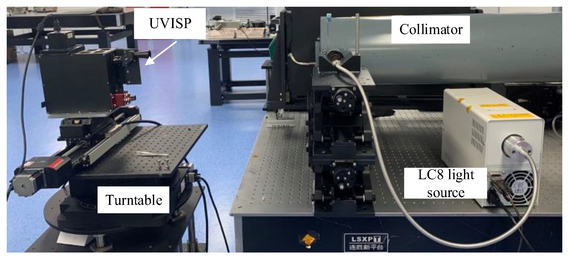
2. Materials and Methods

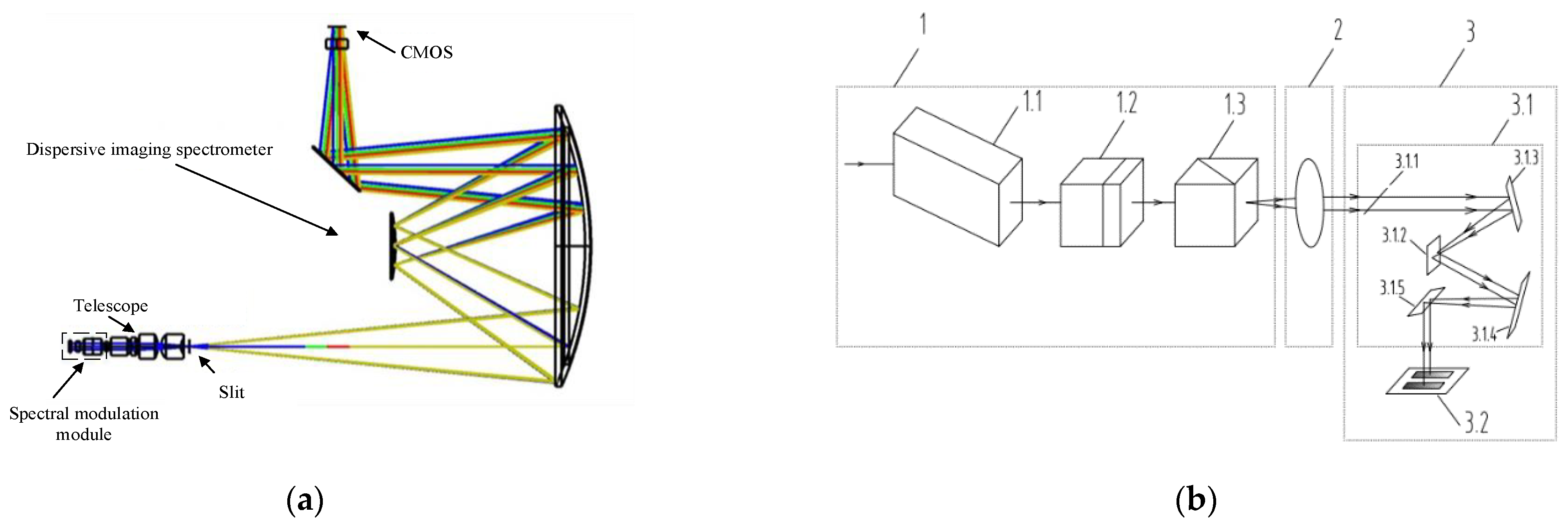
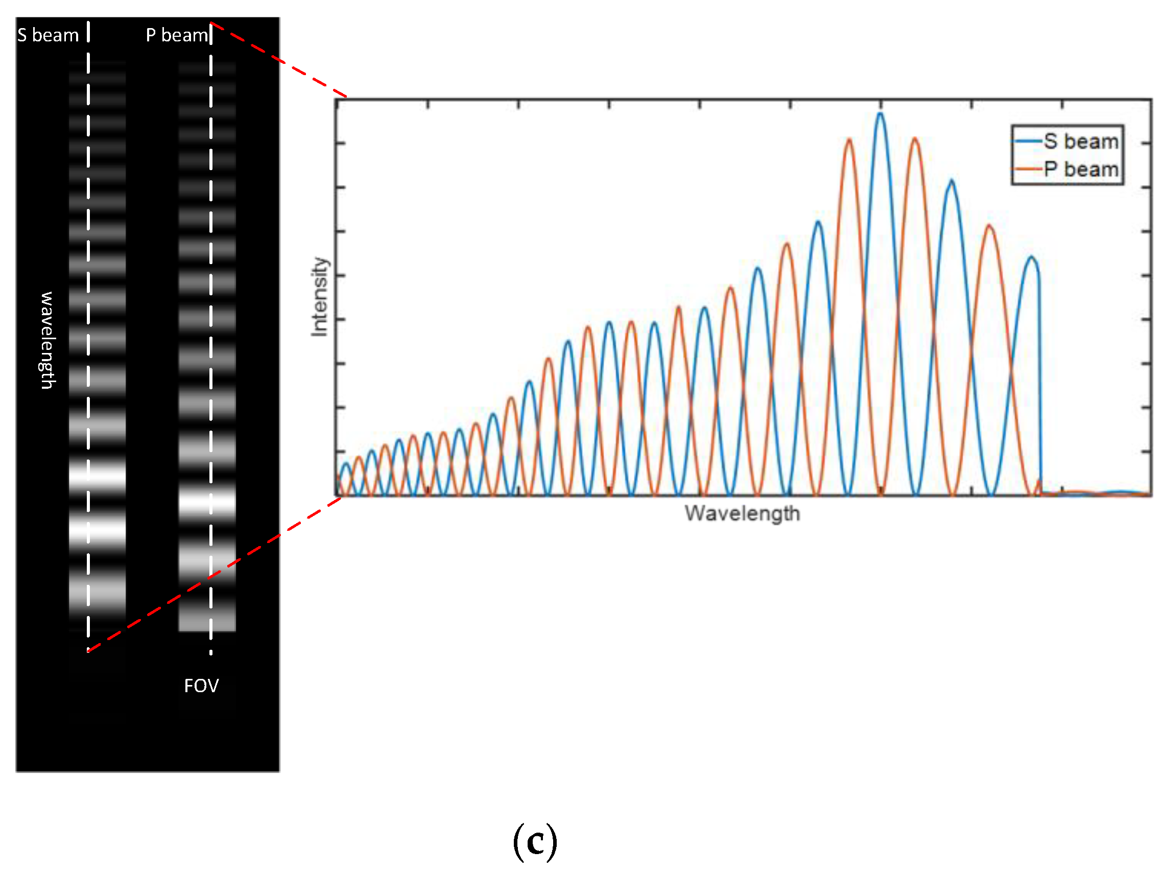
2.1. Instrument Configuration and Radiometric Model

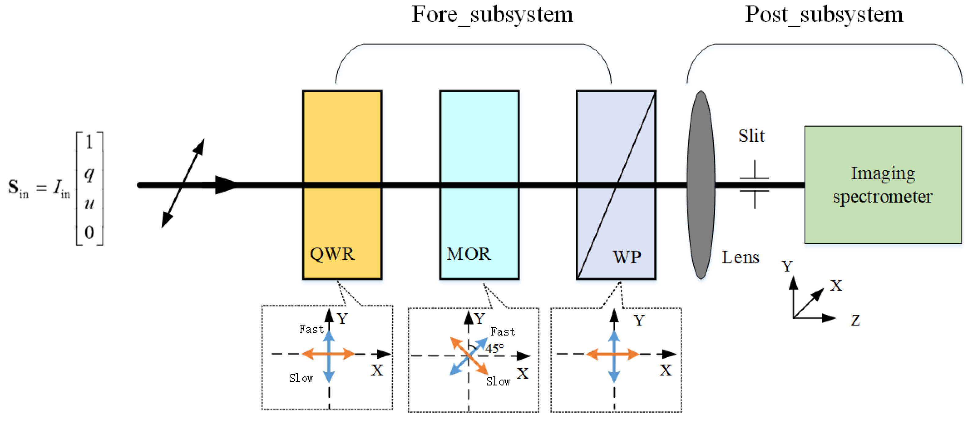
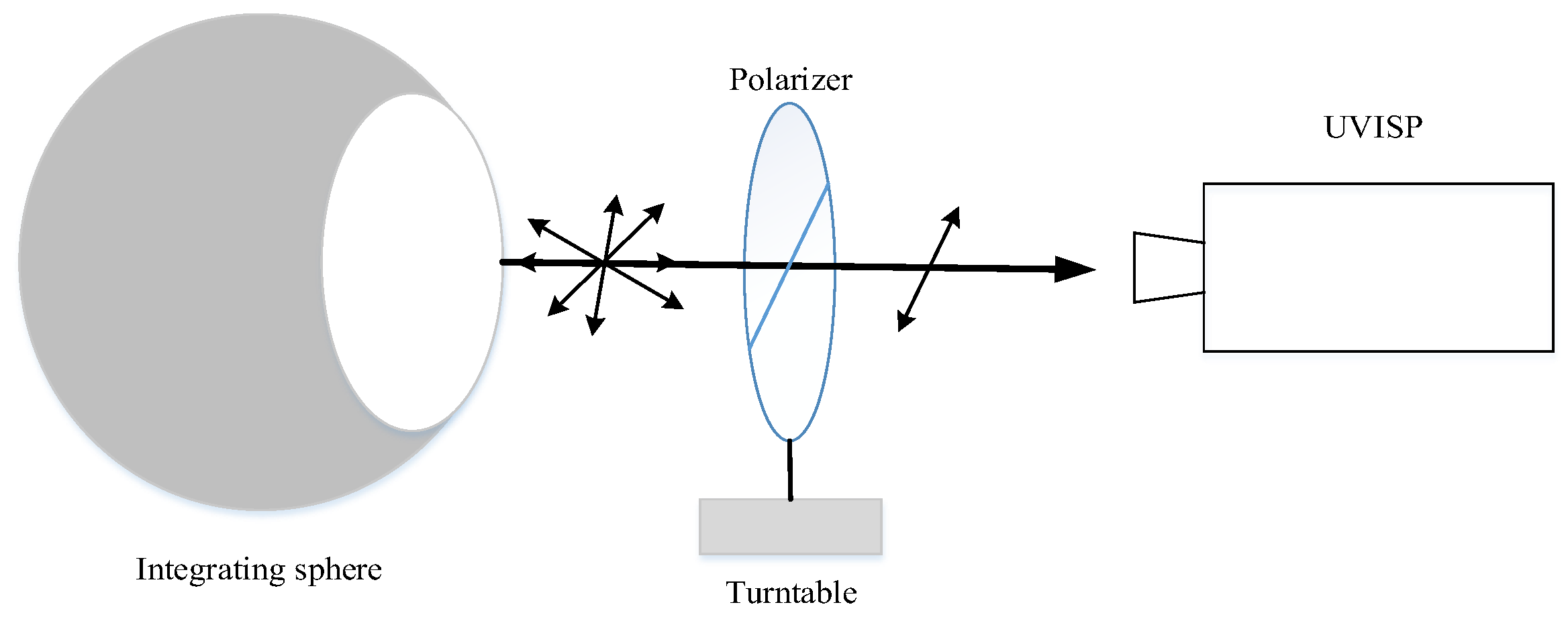
2.1.1. Instrument Configuration

A UVISP is a remote sensing device that can observe the spectral, radiometric, and linear polarimetric characteristics of targets in the ultraviolet–visible band. The optical system is shown in Figure 1. A spectral modulation module (SMM), as the modulator, consists of an achromatic quarter-wave retarder (QWR), a multiple-order retarder (MOR), and a Wollaston prism (WP). The achromatic QWR is a Fresnel Rhomb, which produces a phase shift of π/2 through two total internal reflections. The angle between the fast axis of the QWR and the fast axis MOR is 45°, and the two orthogonally analyzed directions of the WP are parallel and perpendicular to the fast axis of the QWR. After the target light passes through the SMM, the polarization information is encoded as intensity variations in wavelength and is separated into two beams (called the S beam and P beam in this paper) with orthogonal polarization; then, these two beams are imaged on a slit by the front telescope module. The slit is followed by a spectral dispersion system, through which each beam of light from the slit is dispersed and refocused to form a monochromatic image that is received by a 16-bit CMOS detector with a resolution of 2048 × 2048. Figure 1c displays the modulated spectra for the fully polarized light on the detector. In this way, the one-dimensional spatial and spectral information of the target along the slit length direction can be obtained simultaneously in one imaging step, and then the two-dimensional spatial information of the target can be obtained by push-broom imaging perpendicular to the slit length direction. For the UVISP prototype, its detection band ranges from 340 to 520 nm. The field of view (FOV) is ±4°, the column indices of the spatial dimensions of the S beam and P beam are 110–270 (V) and 400–550 (V), respectively, and the row indices of the spectral dimension are 700–1500 (H).

2.1.2. Radiometric Model

The radiometric model of the UVISP describes the response of the instrument to incident radiation. According to the optical design scheme in Section 2.1, the whole measurement system can be divided into two parts: a fore-subsystem and a post-subsystem. A diagram of the simplified measurement system is shown in Figure 2.

The fore-subsystem is an SMM, including QWR, MOR, and WP; the post-subsystem consists of a telescope module and imaging spectrum module. A global coordinate system is established with the horizontal polarization direction parallel and perpendicular to the WP as the X and Y axes and the system optical axis direction as the Z axis. Considering the polarization characteristics of the UVISP, when incident light passes through the system, the Stokes vector of emergent light can be described as

$$S_{\mathrm{out}}={{\rm M}}_{\mathrm{Post}\_\mathrm{sys}}{M}_{\mathrm{Fore}\_\mathrm{sys}}{S}_{\mathrm{in}}$$

(1)

where ${{\rm M}}_{\mathrm{Post}\_\mathrm{sys}}$ and $M_{\mathrm{Fore}\_\mathrm{sys}}$ denote the Müller matrices of the post-subsystem and fore-subsystem, respectively. We set the total radiation to $I_{\mathrm{in}}$, and $S_{\mathrm{in}}=I_{\mathrm{in}}{\left[\begin{array}{cccc}1& q& u& 0\end{array}\right]}^T$ is the Stokes vector of incident linearly polarized light. However, for the SMM, the optical properties of retarders and Wollaston prisms are unsatisfactory because of manufacturing defects and inevitable alignment errors, where the Müller matrix of the QWR with errors is given by

$$M_{\mathrm{QWR}}\left({\alpha }_1,{\phi }_1\right)=\left[\begin{array}{cccc}1& 0& 0& 0\\ 0& {\cos }^2\left(2{\alpha }_1\right)+\cos \left({\phi }_1\right){\sin }^2\left(2{\alpha }_1\right)& \frac{1}{2}\left[1-\cos \left({\phi }_1\right)\right]\sin \left(4{\alpha }_1\right)& \sin \left({\phi }_1\right)\sin \left(2{\alpha }_1\right)\\ 0& \frac{1}{2}\left[1-\cos \left({\phi }_1\right)\right]\sin \left(4{\alpha }_1\right)& {\sin }^2\left(2{\theta }_1\right)+\cos \left({\phi }_1\right){\cos }^2\left(2{\alpha }_1\right)& \sin \left({\phi }_1\right)\cos \left(2{\alpha }_1\right)\\ 0& -\sin \left({\phi }_1\right)\sin \left(2{\alpha }_1\right)& \sin \left({\phi }_1\right)\cos \left(2{\alpha }_1\right)& \cos \left({\phi }_1\right)\end{array}\right]$$

(2)

The Müller matrix of the MOR with errors can be described by

$$M_{\mathrm{MOR}}\left({\alpha }_2,{\phi }_2\right)=\left[\begin{array}{cccc}1& 0& 0& 0\\ 0& {\sin }^2\left(2{\alpha }_2\right)+\cos \left({\phi }_2\right){\cos }^2\left(2{\alpha }_2\right)& -\frac{1}{2}\left[1-\cos \left({\phi }_2\right)\right]\sin \left(4{\alpha }_2\right)& -\sin \left({\phi }_2\right)\cos \left(2{\alpha }_2\right)\\ 0& -\frac{1}{2}\left[1-\cos \left({\phi }_2\right)\right]\sin \left(4{\alpha }_2\right)& {\cos }^2\left(2{\alpha }_2\right)+\cos \left({\phi }_2\right){\sin }^2\left(2{\alpha }_2\right)& -\sin \left({\phi }_2\right)\cos \left(2{\alpha }_2\right)\\ 0& \sin \left({\phi }_2\right)\cos \left(2{\alpha }_2\right)& \sin \left({\phi }_2\right)\sin \left(2{\alpha }_2\right)& \cos \left({\phi }_2\right)\end{array}\right]$$

(3)

The Müller matrix of the WP with errors can be expressed as

$$M_{\mathrm{WP}}\left(\epsilon \right)=\frac{1}{2}\left[\begin{array}{cccc}1& k\frac{\epsilon -1}{\epsilon +1}& 0& 0\\ k\frac{\epsilon -1}{\epsilon +1}& 1& 0& 0\\ 0& 0& \frac{2\sqrt{\epsilon }}{\epsilon +1}& 0\\ 0& 0& 0& \frac{2\sqrt{\epsilon }}{\epsilon +1}\end{array}\right], k=\pm 1$$

(4)

where ${\phi }_1=\frac{\pi }{2}+{\varphi }_1$, ${\phi }_2=\frac{2\pi \delta }{\lambda }$. ${\varphi }_1$ and $\delta$ are the retardance error of the QWR and the actual retardance of the MOR, respectively. ${\alpha }_1$, ${\alpha }_2$, and $\epsilon$ denote the alignment error of the QWR, alignment error of the MOR, and extinction ratio of the WP, respectively. $k=\pm 1$ indicates two orthogonal beams emitted by the WP, where $k=1$ corresponds to the vertical polarized beam, while $k=-1$ corresponds to the horizontally polarized beam. The Müller matrix of the fore-subsystem can be calculated by the following equation:

$$M_{\mathrm{Fore}\_\mathrm{sys}}=M_{\mathrm{WP}}{M}_{\mathrm{MOR}}{M}_{\mathrm{QWR}}$$

(5)

The post-subsystem includes a telescope module and an imaging spectrum module, where the telescope consists of a series of lenses, and the imaging spectrum module is based on the Offner reflective form and consists of mirror groups. According to the Müller matrix property of the lens interface, the equivalent Müller matrix of the telescope module is described as [40]

$$M_{\mathrm{Lens}}=A_{\mathrm{Lens}}\left[\begin{array}{cccc}1& D_{\mathrm{Lens}}& 0& 0\\ D_{\mathrm{Lens}}& 1& 0& 0\\ 0& 0& 1& {\delta }_{\mathrm{Lens}}\\ 0& 0& -{\delta }_{\mathrm{Lens}}& 1\end{array}\right]$$

(6)

where $A_{\mathrm{Lens}}$, $D_{\mathrm{Lens}}$, and ${\delta }_{\mathrm{Lens}}$ denote the transmittance, diattenuation, and retardance of the telescope, respectively. Similarly, the mirror groups in the imaging spectrum module are modeled in the same way as the lenses. According to the Müller matrix properties of the mirror interface, the equivalent Müller matrix can be described as [40]

$$M_{\mathrm{Spec}}=A_{\mathrm{Spec}}\left[\begin{array}{cccc}1& D_{\mathrm{Spec}}& 0& 0\\ D_{\mathrm{Spec}}& 1& 0& 0\\ 0& 0& -1& -{\delta }_{\mathrm{Spec}}\\ 0& 0& {\delta }_{\mathrm{Spec}}& -1\end{array}\right]$$

(7)

where $A_{\mathrm{Spec}}$, $D_{\mathrm{Spec}}$, and ${\delta }_{\mathrm{Spec}}$ denote transmittance, diattenuation, and the retardance of the imaging spectrum module, respectively. We can describe the Müller matrix of the post-subsystem as

$$M_{\mathrm{Post}\_\mathrm{sys}}=M_{\mathrm{Spec}}{M}_{\mathrm{Lens}}$$

(8)

Equations (1), (5) and (8) are combined, and the spectral radiance of the modulated spectrum can be obtained by extracting the first element of $S_{\mathrm{out}}$:

$$I_{\mathrm{s}}=\frac{1}{2}{I}_{\mathrm{in}}{A}_{\mathrm{Lens}}{A}_{\mathrm{Spec}}\left(p_{11}+p_{12}\right)\left\{\begin{array}{l}1+\frac{\epsilon -1}{\epsilon +1}\left[{\mathrm{\Gamma }}_1\cos \left(\frac{2\pi \delta }{\lambda }\right)+{\mathrm{\Gamma }}_2\sin \left(\frac{2\pi \delta }{\lambda }\right)+{\mathrm{\Gamma }}_3\right]q\\ +\frac{\epsilon -1}{\epsilon +1}\left[{\mathrm{\Gamma }}_4\cos \left(\frac{2\pi \delta }{\lambda }\right)+{\mathrm{\Gamma }}_5\sin \left(\frac{2\pi \delta }{\lambda }\right)+{\mathrm{\Gamma }}_6\right]u\end{array}\right\}$$

(9)

$$I_{\mathrm{p}}=\frac{1}{2}{I}_{\mathrm{in}}{A}_{\mathrm{Lens}}{A}_{\mathrm{Spec}}\left(p_{11}-p_{12}\right)\left\{\begin{array}{l}1-\frac{\epsilon -1}{\epsilon +1}\left[{\mathrm{\Gamma }}_1\cos \left(\frac{2\pi \delta }{\lambda }\right)+{\mathrm{\Gamma }}_2\sin \left(\frac{2\pi \delta }{\lambda }\right)+{\mathrm{\Gamma }}_3\right]q\\ -\frac{\epsilon -1}{\epsilon +1}\left[{\mathrm{\Gamma }}_4\cos \left(\frac{2\pi \delta }{\lambda }\right)+{\mathrm{\Gamma }}_5\sin \left(\frac{2\pi \delta }{\lambda }\right)+{\mathrm{\Gamma }}_6\right]u\end{array}\right\}$$

(10)

where $I_{\mathrm{s}}$ and $I_{\mathrm{p}}$ denote the vertically polarized beam and horizontally polarized beam, respectively. $p_{11}=1+D_{\mathrm{Spec}}{D}_{\mathrm{Lens}}$, $p_{12}=D_{\mathrm{Spec}}+D_{\mathrm{Lens}}$. ${\mathrm{\Gamma }}_{\mathrm{k}}\left(\mathrm{k}=1,2,\dots ,6\right)$ represents the error factors of the fore-subsystem, which can be described as

$$\{\begin{array}{l}{\mathrm{\Gamma }}_1=c^2\left(b^2-a^{2}f\right)+\left(1+f\right)abcd\\ {\mathrm{\Gamma }}_2=ace\\ {\mathrm{\Gamma }}_3=d^2\left(b^2-a^{2}f\right)-\left(1+f\right)abcd\\ {\mathrm{\Gamma }}_4=\left(1+f\right)ab{c}^2+cd\left(-b^{2}f+a^2\right)\\ {\mathrm{\Gamma }}_5=-bce\\ {\mathrm{\Gamma }}_6=d^2\left(1+f\right)ab-cd\left(-b^{2}f+a^2\right)\end{array}$$

(11)

where $a=\sin 2{\alpha }_1$, $b=\cos 2{\alpha }_1$, $c=\cos 2{\alpha }_2$, $d=\sin 2{\alpha }_2$, $e=\cos {\varphi }_1$, and $f=\sin {\varphi }_1$.

We can describe the polarization effect of the subsystem using a Müller matrix, and the effect of the point spread function of the imaging spectrum module also needs consideration. In fact, the spectra recorded by the spectrometer can be seen as the convolution of the modulated spectrum with the spectral spread function. The convolved spectrum is expressed as

$$I_{\mathrm{s}/\mathrm{p}}^{\prime }\left({\lambda }_i\right)={\displaystyle {\int }_0^{+\infty }{I}_{\mathrm{s}/\mathrm{p}}\left(\lambda \right)}P\left(\lambda -{\lambda }_i\right)d\lambda =I_{\mathrm{s}/\mathrm{p}}\left({\lambda }_i\right)\ast P\left({\lambda }_i\right)$$

(12)

$$P(\lambda -{\lambda }_i)=K\exp \left[-\frac{1}{2}{\left(\frac{\lambda -{\lambda }_i}{{\sigma }_i}\right)}^2\right]$$

(13)

where ∗ denotes the convolution symbol, $K$ is a constant, ${\lambda }_i$ is the central wavelength, ${\sigma }_i$ is the standard deviation of the Gaussian curve, and $P\left(\lambda \right)$ is the spectral spread function. In this paper, we assume that the Stokes parameters of incident light are spectrally smooth, so $I_{\mathrm{in}}$, $q$, and $u$ remain unchanged after convolving with $P\left(\lambda \right)$. However, the modulation amplitude of the sinusoidal carrier and cosine carrier will decrease because of spectral broadening. Additionally, the imaging quality of the S beam and P beam in the post-subsystem is different due to the influence of the optical system distortion, which causes variations in $P\left(\lambda \right)$. Thus, the modulation amplitudes of the S beam and P beam are different. We can obtain the convolved spectra as follows by combining Equations (9), (10) and (12):

$$I^{\prime }{}_{\mathrm{s}}\left(\lambda \right)=\frac{1}{2}{I}_{\mathrm{in}}\left(\lambda \right)A_{\mathrm{Lens}}{A}_{\mathrm{Spec}}\left(p_{11}+p_{12}\right)\left\{\begin{array}{l}1+\frac{\epsilon -1}{\epsilon +1}\left[W_{\mathrm{s}}\left(\lambda \right){\mathrm{\Gamma }}_1\cos \left(\frac{2\pi \delta }{\lambda }\right)+W_{\mathrm{s}}\left(\lambda \right){\mathrm{\Gamma }}_2\sin \left(\frac{2\pi \delta }{\lambda }\right)+{\mathrm{\Gamma }}_3\right]q\\ +\frac{\epsilon -1}{\epsilon +1}\left[W_{\mathrm{s}}\left(\lambda \right){\mathrm{\Gamma }}_4\cos \left(\frac{2\pi \delta }{\lambda }\right)+W_{\mathrm{s}}\left(\lambda \right){\mathrm{\Gamma }}_5\sin \left(\frac{2\pi \delta }{\lambda }\right)+{\mathrm{\Gamma }}_6\right]u\end{array}\right\}$$

(14)

$$I^{\prime }{}_{\mathrm{p}}\left(\lambda \right)=\frac{1}{2}{I}_{\mathrm{in}}\left(\lambda \right)A_{\mathrm{Lens}}{A}_{\mathrm{Spec}}\left(p_{11}-p_{12}\right)\left\{\begin{array}{l}1-\frac{\epsilon -1}{\epsilon +1}\left[W_{\mathrm{p}}\left(\lambda \right){\mathrm{\Gamma }}_1\cos \left(\frac{2\pi \delta }{\lambda }\right)+W_{\mathrm{p}}\left(\lambda \right){\mathrm{\Gamma }}_2\sin \left(\frac{2\pi \delta }{\lambda }\right)+{\mathrm{\Gamma }}_3\right]q\\ -\frac{\epsilon -1}{\epsilon +1}\left[W_{\mathrm{p}}\left(\lambda \right){\mathrm{\Gamma }}_4\cos \left(\frac{2\pi \delta }{\lambda }\right)+W_{\mathrm{p}}\left(\lambda \right){\mathrm{\Gamma }}_5\sin \left(\frac{2\pi \delta }{\lambda }\right)+{\mathrm{\Gamma }}_6\right]u\end{array}\right\}$$

(15)

where $W_{\mathrm{s}}$ and $W_{\mathrm{p}}$ denote the modulation amplitudes of the S beam and P beam, respectively, proposed by the SPEX polarimeter [38,41], which are used to characterize the effect of spectral broadening of the spectrometer. From Equations (14) and (15), we can see that the retardance in the telescope module and imaging spectrum module has no effect on the modulated spectrum, and the diattenuation can be regarded as part of the relative response coefficient of the modulation spectrum. If the linear response of the detector is good, the relationship between the spectral radiation received by the detector and the output digital number (DN) value $C_{\mathrm{s}}$, $C_{\mathrm{p}}$ can be obtained.

$$C_{\mathrm{s}}\left(\lambda \right)=\frac{1}{2}{A}_{\mathrm{s}}{I}_{in}\left\{\begin{array}{l}1+\frac{\epsilon -1}{\epsilon +1}\left[W_{\mathrm{s}}\left(\lambda \right){\mathrm{\Gamma }}_1\cos \left(\frac{2\pi \delta }{\lambda }\right)+W_{\mathrm{s}}\left(\lambda \right){\mathrm{\Gamma }}_2\sin \left(\frac{2\pi \delta }{\lambda }\right)+{\mathrm{\Gamma }}_3\right]q\\ +\frac{\epsilon -1}{\epsilon +1}\left[W_{\mathrm{s}}\left(\lambda \right){\mathrm{\Gamma }}_4\cos \left(\frac{2\pi \delta }{\lambda }\right)+W_{\mathrm{s}}\left(\lambda \right){\mathrm{\Gamma }}_5\sin \left(\frac{2\pi \delta }{\lambda }\right)+{\mathrm{\Gamma }}_6\right]u\end{array}\right\}+D_{\mathrm{s}}$$

(16)

$$C_{\mathrm{p}}\left(\lambda \right)=\frac{1}{2}{A}_{\mathrm{p}}{I}_{in}\left\{\begin{array}{l}1-\frac{\epsilon -1}{\epsilon +1}\left[W_{\mathrm{p}}\left(\lambda \right){\mathrm{\Gamma }}_1\cos \left(\frac{2\pi \delta }{\lambda }\right)+W_{\mathrm{p}}\left(\lambda \right){\mathrm{\Gamma }}_2\sin \left(\frac{2\pi \delta }{\lambda }\right)+{\mathrm{\Gamma }}_3\right]q\\ -\frac{\epsilon -1}{\epsilon +1}\left[W_{\mathrm{p}}\left(\lambda \right){\mathrm{\Gamma }}_4\cos \left(\frac{2\pi \delta }{\lambda }\right)+W_{\mathrm{p}}\left(\lambda \right){\mathrm{\Gamma }}_5\sin \left(\frac{2\pi \delta }{\lambda }\right)+{\mathrm{\Gamma }}_6\right]u\end{array}\right\}+D_{\mathrm{p}}$$

(17)

where $D_{\mathrm{s}}$, $D_{\mathrm{p}}$ denote the dark signal of the detector, and

$$A_s=A{A}_{\mathrm{Lens}}\left(\lambda \right)A_{\mathrm{Spec}}\left(\lambda \right)\left(p_{11}+p_{12}\right)$$

(18)

$$A_p=A{A}_{\mathrm{Lens}}\left(\lambda \right)A_{\mathrm{Spec}}\left(\lambda \right)\left(p_{11}-p_{12}\right)$$

(19)

where $A_s$ and $A_{\mathrm{p}}$ denote the radiometric calibration coefficients, and $A$ represents the pixel response of the detector. By sorting out Equations (16) and (17), the radiometric model of the UVISP can be written into the linear superposition form of each component in the Stokes vector of the incident light

$$C_{\mathrm{s}}\left(\lambda \right)=\frac{1}{2}{A}_{\mathrm{s}}{I}_{\mathrm{in}}\left(\lambda \right)\left[1+q{m}_{11}\left(\lambda \right)+u{m}_{12}\left(\lambda \right)\right]+D_{\mathrm{s}}$$

(20)

$$C_{\mathrm{p}}\left(\lambda \right)=\frac{1}{2}{A}_{\mathrm{p}}{I}_{\mathrm{in}}\left(\lambda \right)\left[1+q{m}_{21}\left(\lambda \right)+u{m}_{22}\left(\lambda \right)\right]+D_{\mathrm{p}}$$

(21)

where

$$\{\begin{array}{l}{m}_{11}\left(\lambda \right)=\frac{\epsilon -1}{\epsilon +1}\left[W_{\mathrm{s}}\left(\lambda \right){\mathrm{\Gamma }}_1\cos \left(\frac{2\pi \delta }{\lambda }\right)+W_{\mathrm{s}}\left(\lambda \right){\mathrm{\Gamma }}_2\sin \left(\frac{2\pi \delta }{\lambda }\right)+{\mathrm{\Gamma }}_3\right]\\ m_{12}\left(\lambda \right)=\frac{\epsilon -1}{\epsilon +1}\left[W_{\mathrm{s}}\left(\lambda \right){\mathrm{\Gamma }}_4\cos \left(\frac{2\pi \delta }{\lambda }\right)+W_{\mathrm{s}}\left(\lambda \right){\mathrm{\Gamma }}_5\sin \left(\frac{2\pi \delta }{\lambda }\right)+{\mathrm{\Gamma }}_6\right]\end{array}$$

(22)

$$\{\begin{array}{l}{m}_{21}\left(\lambda \right)=-\frac{\epsilon -1}{\epsilon +1}\left[W_{\mathrm{p}}\left(\lambda \right){\mathrm{\Gamma }}_1\cos \left(\frac{2\pi \delta }{\lambda }\right)+W_{\mathrm{p}}\left(\lambda \right){\mathrm{\Gamma }}_2\sin \left(\frac{2\pi \delta }{\lambda }\right)+{\mathrm{\Gamma }}_3\right]\\ m_{22}\left(\lambda \right)=-\frac{\epsilon -1}{\epsilon +1}\left[W_{\mathrm{p}}\left(\lambda \right){\mathrm{\Gamma }}_4\cos \left(\frac{2\pi \delta }{\lambda }\right)+W_{\mathrm{p}}\left(\lambda \right){\mathrm{\Gamma }}_5\sin \left(\frac{2\pi \delta }{\lambda }\right)+{\mathrm{\Gamma }}_6\right]\end{array}$$

(23)

Assuming that the performance of the optic system is ideal, the polarimetric coefficients are

$$\{\begin{array}{l}{m}_{11}\left(\lambda \right)=-m_{21}\left(\lambda \right)=\cos \left(\frac{2\pi \delta }{\lambda }\right)\\ m_{12}\left(\lambda \right)=-m_{22}\left(\lambda \right)=\sin \left(\frac{2\pi \delta }{\lambda }\right)\end{array}$$

(24)

The only parameter introduced by the SMM is the retardance $\delta$.

2.2. Calibration Methods of UVISP

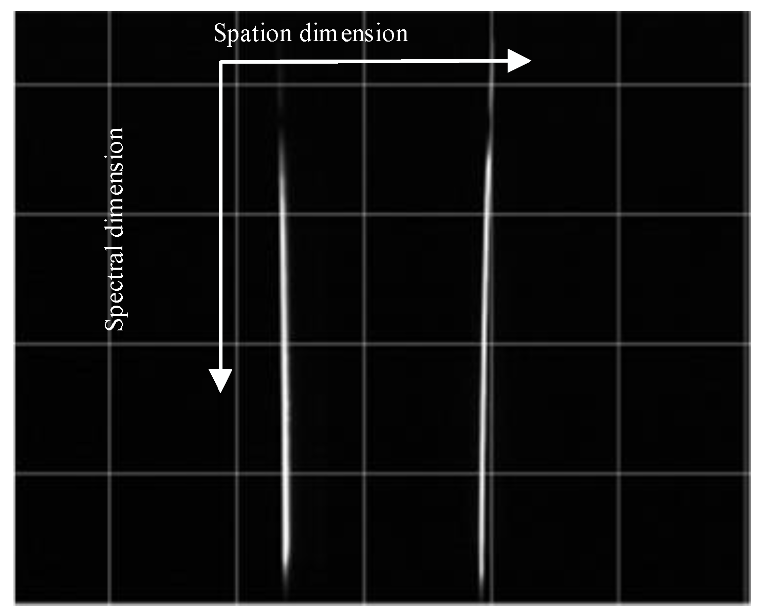
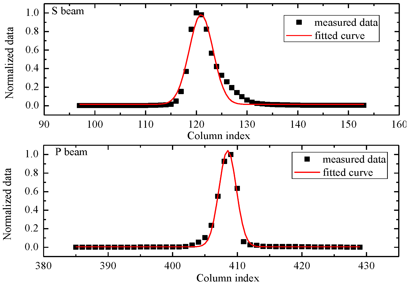
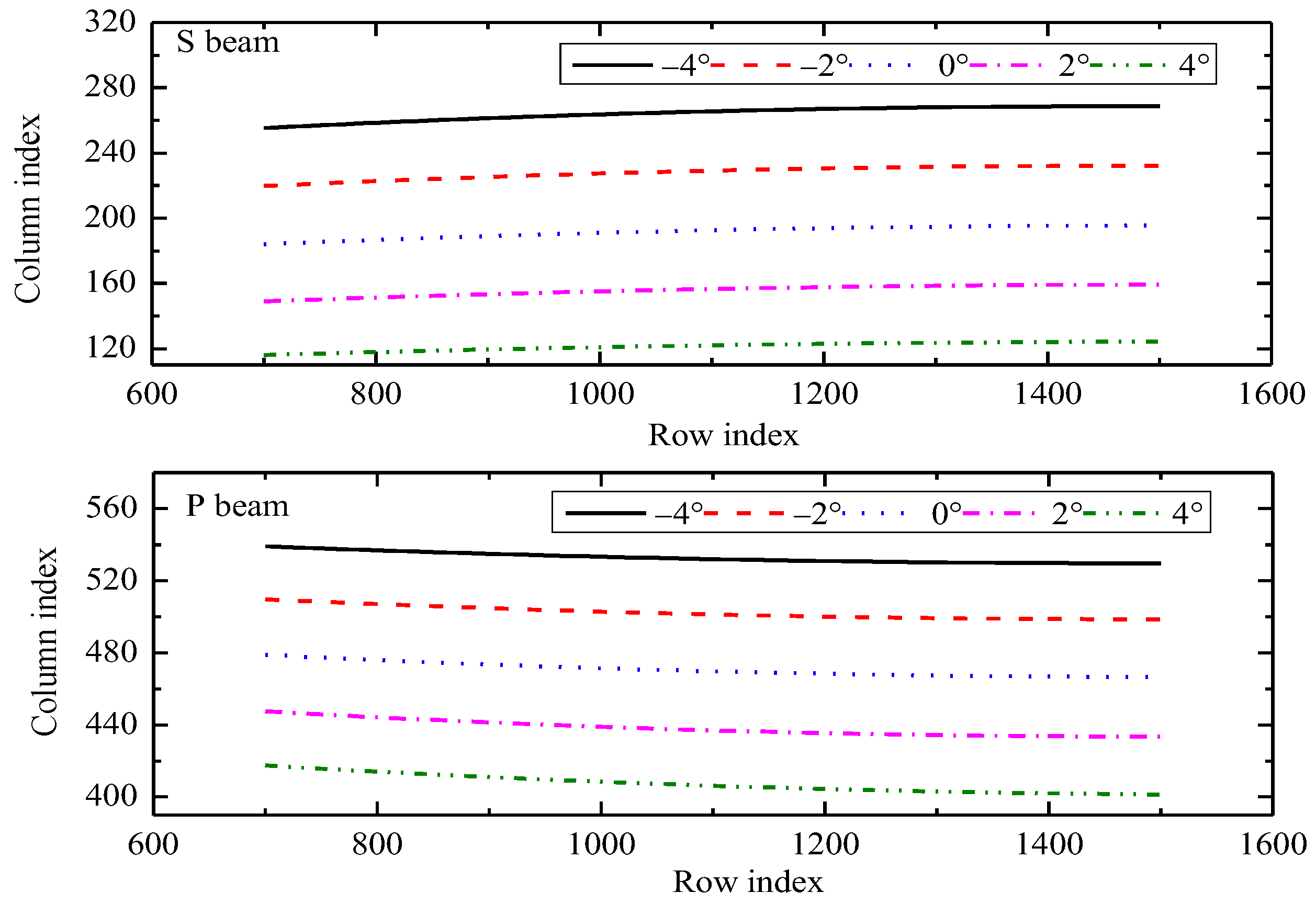
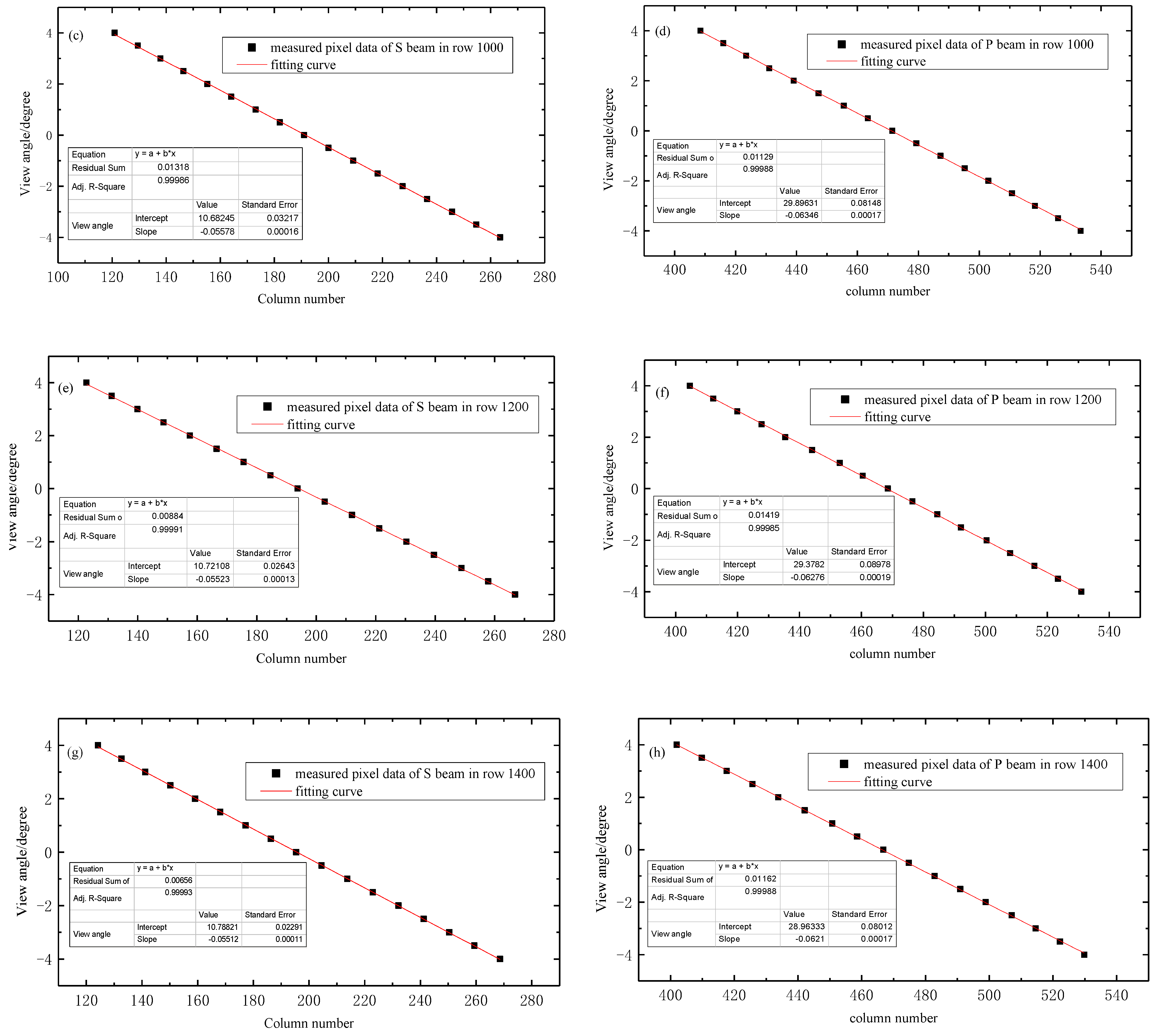
2.2.1. Geometric Calibration Principle

Ideally, the spectral lines of a fixed FOV should be distributed in the same column on the UVISP detector. However, because the SMM uses the WP as an analyzer, the dispersion effect of WP causes the splitting angles of various wavelengths to be slightly different, resulting in a spectrum that is slanted for a particular FOV. In addition, to accurately demodulate the polarization information, pairs of spectra of the S beam and P beam with a common FOV should be extracted from raw image data (the demodulation method is described in Section 2.3). Thus, precision matching is essential for the S beam and P beam to eliminate spurious demodulated polarization information.

The first step in the calibration processing is geometric calibration, which assigns the FOV angles of the UVISP to detector pixels. When illuminating the instrument using parallel light, the detector records two spectral lines of the S beam and P beam, which contain a collection of detector pixels with a common view angle. Usually, the point spread function of the spectrometer is in Gaussian form; thus for the pixels in a fixed row, a Gaussian function is used to fit the DN to determine the column number of maximum, and the view angle is assigned to the column pixel. This procedure is performed for all row pixels of the S beam and P beam. For a general spectrometer, the field of view angle $\theta$ and column pixel number $m$ can be fitted by polynomials. Combining the measurement results of UVISP under specific observation angles, then we can use the least square method to obtain the fitting coefficients. In this paper, a first-order polynomial fitting procedure is introduced as an example. For the pixels in row $i$ of the detector, the linear regression model is as follows:

$${\theta }_{im}\left(X_{im}\right)={\partial }_0+{\partial }_1{X}_{im}$$

(25)

where ${\partial }_0$ and ${\partial }_1$ are the regression coefficients, and $X_{im}$ is the regression variable. Assuming that there are N groups of measurement data, the regression coefficients can be derived as follows:

$$\{\begin{array}{l}{\partial }_1=\frac{{\displaystyle \sum _{i=1}^N\left(X_{im}-\overline{X_i}\right)\left({\theta }_{im}-\overline{{\theta }_i}\right)}}{{\displaystyle \sum _{i=1}^N{\left(X_{im}-\overline{X_i}\right)}^2}}\\ {\partial }_0=\overline{{\theta }_{\mathrm{i}}}-{\partial }_1\overline{X_i}\\ \overline{X_i}=\frac{1}{N}{\displaystyle \sum _{m=1}^N{X}_{im}}\\ \overline{{\theta }_{\mathrm{i}}}=\frac{1}{N}{\displaystyle \sum _{m=1}^N{\theta }_{im}}\end{array}$$

(26)

$R^2$ is used to evaluate how well the measured data are explained by the model [39]

$$R^2=1-\frac{{\displaystyle \sum _{i=1}^N{\left(y_i-\widehat{y}\right)}^2}}{{\displaystyle \sum _{i=1}^N{\left(y_i-\overline{y}\right)}^2}}$$

(27)

where $y_i$ and $\widehat{y}$ denote the sampled data and model estimate, respectively, and $\overline{y}$ is the mean of the sampled data. A larger $R^2$ value indicates a better correlation between the data and the model. $R^2=1$ indicates an ideal fit, and $R^2=0$ indicates no correlation.

The data processing method is identical for each row of pixels. To extract the spectra of the S beam and P beam at a given FOV, the collection of pixels $\left\{m_{\mathrm{s}}\left[i\right],i\right\},\left\{m_{\mathrm{p}}\left[i\right],i\right\},i=700:1500$ is presented to describe the spectral line distributions in the detector, where $m_{\mathrm{s}}$ and $m_{\mathrm{p}}$ are the pixel column numbers of the S beam and P beam, respectively.

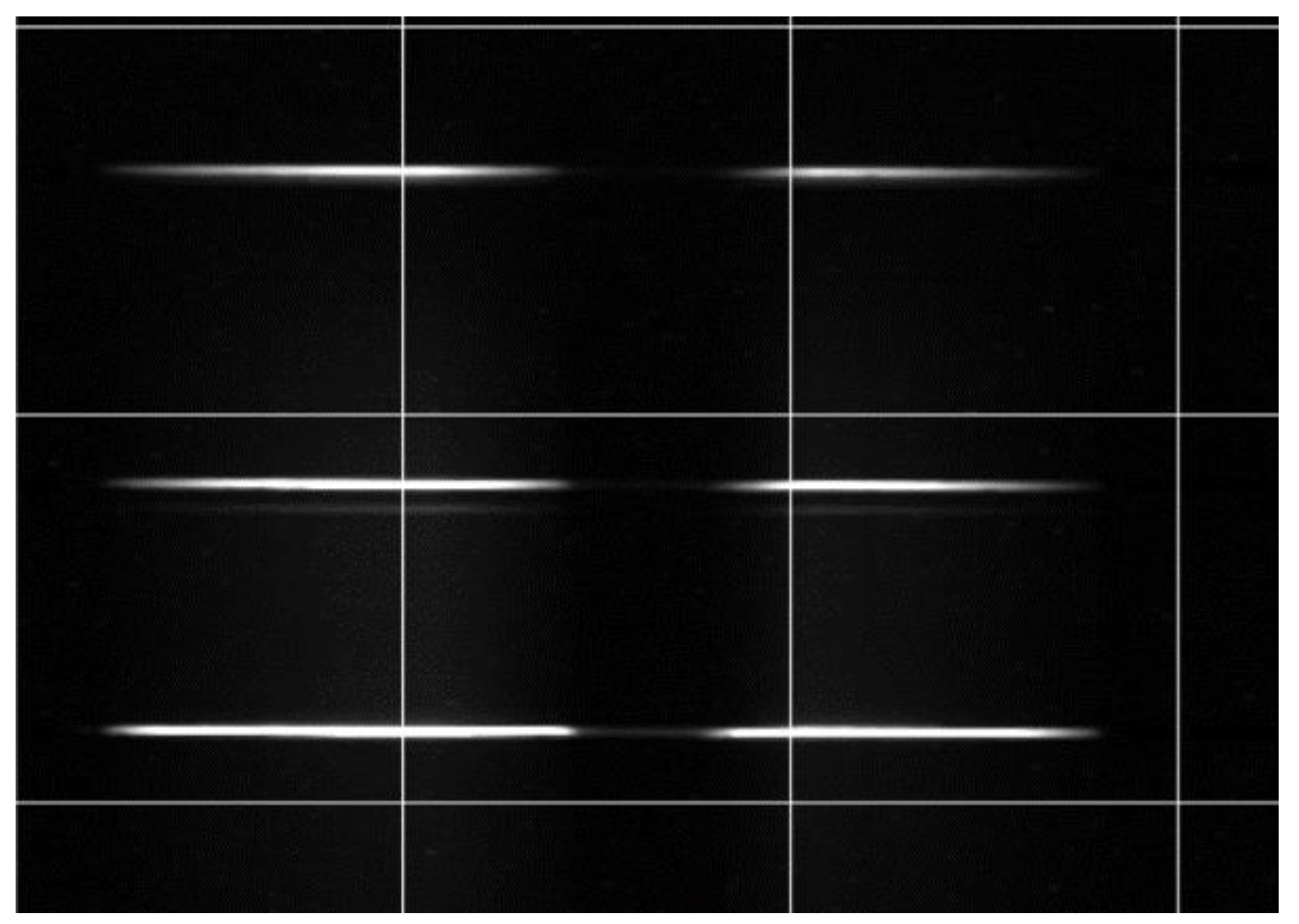
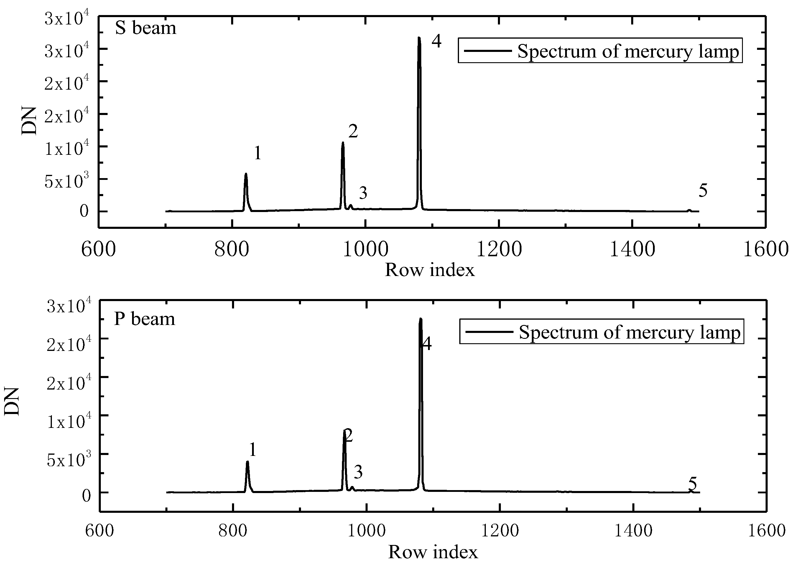
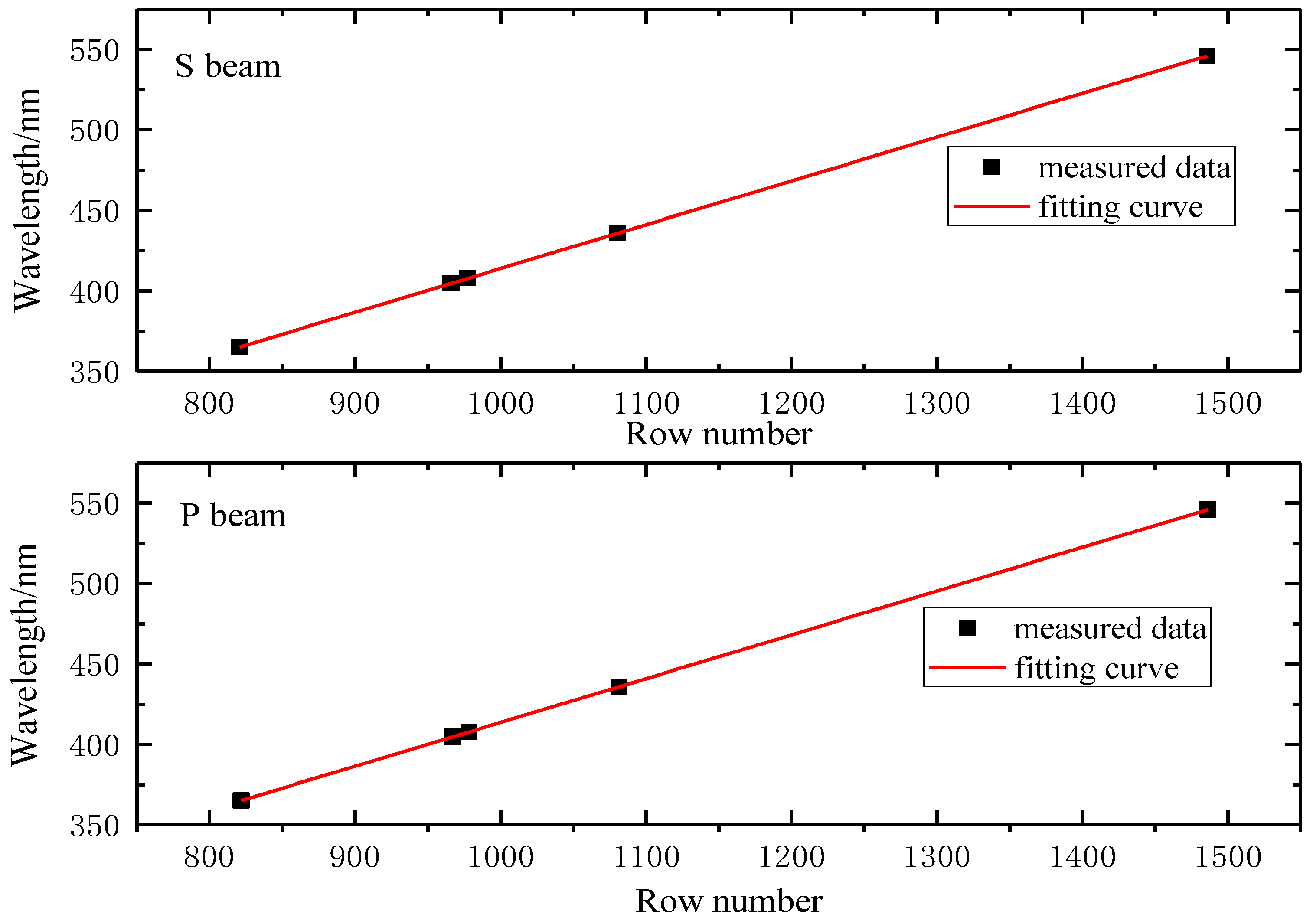
2.2.2. Spectral Calibration Principle and Spectral Matching

Spectral calibration of the UVISP is conducted mainly to determine the central wavelength distribution and spectral range of the instrument. Unlike the general spectrometer, for UVISP, spectral calibration is conducted for each S spectrum and P spectrum pair at a given FOV.

Since the row number of pixels and the wavelength approximately meet the linear relationship, for the pixels in the extracted spectral line (the pixels collection extracted by the method in Section 2.2.1), the linear regression model can be established as follows:

$${\lambda }_{im}\left(Y_{im}\right)=a+b{Y}_{im}$$

(28)

where $a$ and $b$ are the regression coefficients, and ${\lambda }_{im}$ and $Y_{im}$ represent the central wavelength and row number of pixels, respectively, while the regression coefficients are solved in the same way as in Section 2.2.1.

When the geometric and spectral calibrations are complete, the S spectrum and P spectrum pairs can be obtained from a raw image. For a particular FOV, the pixel collectors of the S beam and P beam can be determined from geometric calibration and are expressed as $\left\{m_{\mathrm{s}}\left[i\right],i\right\}$ and $\left\{m_{\mathrm{p}}\left[i\right],i\right\}$, $i=700,\dots ,1500$. The output result of matched spectra is a pair of arrays $S_{\mathrm{s}/\mathrm{p}}\left[i\right],i=700,\dots ,1500$ with DN. Then, the wavelengths are collected from spectral calibration and assigned to the pairs of spectral arrays. However, the assigned wavelengths of the given FOV for the S beam and P beam are different due to the optical distortion of the spectrometer optical system. To avoid false polarization information generated by demodulation, the sampling wavelengths of the modulated spectrum for the S beam and P beam must be consistent. Therefore, the linear interpolation method is used to resample the spectra of the P beam to complete wavelength matching, and the final matching spectra are $S_{\mathrm{s}/\mathrm{p}}\left[{\lambda }_i\right]$. This spectral extraction and matching process of the raw image is performed for all FOVs.

2.2.3. Radiometric Calibration Principle

In the detecting band, the UVISP displays varied responses to monochromatic light at different wavelengths. On the one hand, there are differences in the response of detector pixels to photons due to the limitations of the detector manufacturing process. On the other hand, different optical components in the optical system have different transmissions to incident light, such as polarization components in the spectral modulation module and glass components in the imaging mirror group, as well as diffraction grating and mirror groups in the spectrometer module. While, based on the demodulation method, the modulated spectrum needs to be normalized by the summary of two orthogonal modulation spectra, it is essential to correct the response difference between the S beam and P beam. Therefore, it is necessary to implement the radiometric correction of UVISP by means of radiometric calibration.

The purpose of radiometric calibration is to establish a quantitative relationship between the instrument output signal and the input spectral radiance. When the incident light of the instrument is nonpolarized, the elements in the Stokes vector of the incident light are zero except for the intensity component. According to Equations (20) and (21), the expression of the radiation calibration equation can be obtained, as shown in Equation (29).

$$\{\begin{array}{l}{C}_{\mathrm{s}}=\frac{1}{2}{A}_{\mathrm{s}}{I}_{\mathrm{in}}\\ C_{\mathrm{p}}=\frac{1}{2}{A}_{\mathrm{p}}{I}_{\mathrm{in}}\end{array}$$

(29)

As seen in Equation (29), radiometric calibration can be achieved with a single uniform light source of known radiance when the instrument response satisfies a linear relationship. However, in practice, due to the instability of the calibration source, the noise of the detector, and the stray light of the instrument, the response of the instrument is not an ideal linear relationship. Using the measurements of multiple known radiance levels of the spectrum, and then a linear fit at each wavelength, we can establish the following fit relationship:

$$\{\begin{array}{l}{C}_{\mathrm{s},\lambda }=\frac{1}{2}{A}_{\mathrm{s},\lambda }{I}_{\lambda }+{\epsilon }_{\mathrm{s},\lambda }\\ C_{\mathrm{p},\lambda }=\frac{1}{2}{A}_{\mathrm{p},\lambda }{I}_{\lambda }+{\epsilon }_{\mathrm{p},\lambda }\end{array}$$

(30)

where $A_{\mathrm{s},\lambda }$, $A_{\mathrm{p},\lambda }$ denote the radiometric calibration coefficients; $C_{\mathrm{s},\lambda }$, $C_{\mathrm{p},\lambda }$ represent the output DN of UVISP at wavelength $\lambda$; $I_{\lambda }$ is the incident light spectrum radiance; and ${\epsilon }_{\mathrm{s},\lambda }$, ${\epsilon }_{\mathrm{p},\lambda }$ denote the biases of S beam and P beam caused by the calibration source and stray light, respectively.

2.2.4. Polarimetric Calibration Principle

From Equations (20) and (21), we know that the polarimetric coefficients $m_{11}$, $m_{12}$, $m_{21}$, $m_{22}$ and the radiometric coefficients describe the response of the instrument to the incident polarized light. The radiometric coefficients can be obtained by the radiation calibration method proposed in Section 2.2.3. $m_{11}$, $m_{12}$, $m_{21}$, and $m_{22}$ are the modulation of Stokes parameters q and u of the S beam and P beam, respectively, which contain modulation carrier and system error information and are determined by system hardware parameters. If the system design and installation are completed, the corresponding polarimetric coefficients will not change. Therefore, to demodulate the polarization information in the modulated spectrum, the polarimetric calibration routine must be implemented to accurately solve the polarimetric coefficients.

To determine the polarimetric coefficients, we use the 100% linearly polarized light with fixed AoLP as the calibration source. The polarized light can be expressed as

$$S=I_{\mathrm{ref}}\left(\lambda \right){\left[1,\cos 2\beta ,\sin \beta ,0\right]}^T$$

(31)

where $\beta$ and $I_{\mathrm{ref}}$ represent the AoLP and spectral radiance of incident light, respectively. According to the radiometric model and combined with the radiometric calibration coefficient, the radiances of the S beam and P beam recorded by the UVISP are calculated as

$$\begin{array}{ll}{I}_{\mathrm{s}}\left(\lambda \right)& =\frac{1}{2}\left[I_{\mathrm{ref}}\left(\lambda \right)+I_{\mathrm{ref}}\left(\lambda \right)m_{11}\left(\lambda \right)\cos \left(2\beta \right)+I_{\mathrm{ref}}\left(\lambda \right)m_{12}\left(\lambda \right)\sin \left(2\beta \right)\right]\\ & =\frac{1}{2}\left[M_{11}\left(\lambda \right)+M_{12}\left(\lambda \right)\cos \left(2\beta \right)+M_{13}\left(\lambda \right)\sin \left(2\beta \right)\right]\end{array}$$

(32)

$$\begin{array}{ll}{I}_{\mathrm{p}}\left(\lambda \right)& =\frac{1}{2}\left[I_{\mathrm{ref}}\left(\lambda \right)+I_{\mathrm{ref}}\left(\lambda \right)m_{21}\left(\lambda \right)\cos \left(2\beta \right)+I_{\mathrm{ref}}\left(\lambda \right)m_{21}\left(\lambda \right)\sin \left(2\beta \right)\right]\\ & =\frac{1}{2}\left[M_{21}\left(\lambda \right)+M_{22}\left(\lambda \right)\cos \left(2\beta \right)+M_{23}\left(\lambda \right)\sin \left(2\beta \right)\right]\end{array}$$

(33)

When the azimuth of the polarizer is varied at equal intervals, we can obtain a series of modulated spectra. For a fixed wavelength ${\lambda }_0$, the least squares fitting method is used to minimize the mean square difference between the fitting values $I_{\mathrm{s},i}$, $I_{\mathrm{p},i}$ and the measured values $y_{\mathrm{s},i}$, $y_{\mathrm{p},i}$, thus we can obtain the values of the coefficients $M_{11}$, $M_{12}$, $M_{21}$ and $M_{22}$. The fitting models are as follows:

$$X_1^2={{\displaystyle \sum _{i=1}^N\left[I_{\mathrm{s},i}-y_{\mathrm{s},i}\right]}}^2$$

(34)

$$X_2^2={{\displaystyle \sum _{i=1}^N\left[I_{\mathrm{p},i}-y_{\mathrm{p},i}\right]}}^2$$

(35)

where N indicates that N groups of data are used for fitting. We can calculate the polarimetric coefficients as follows:

$$\{\begin{array}{l}{m}_{11}\left({\lambda }_0\right)=\frac{M_{12}\left({\lambda }_0\right)}{M_{11}\left({\lambda }_0\right)}\\ m_{12}\left({\lambda }_0\right)=\frac{M_{13}\left({\lambda }_0\right)}{M_{11}\left({\lambda }_0\right)}\end{array}$$

(36)

$$\{\begin{array}{l}{m}_{21}\left({\lambda }_0\right)=\frac{M_{22}\left({\lambda }_0\right)}{M_{21}\left({\lambda }_0\right)}\\ m_{22}\left({\lambda }_0\right)=\frac{M_{23}\left({\lambda }_0\right)}{M_{21}\left({\lambda }_0\right)}\end{array}$$

(37)

2.3. Demodulation Method

Based on the geometric and spectral calibration results, we can pair the S and P spectra precisely and then use the radiometric calibration equation to achieve the radiometric correction of the two orthogonal spectra. The radiance of S and P spectra can be expressed as

$$\{\begin{array}{l}{I}_{\mathrm{s}}\left(\lambda \right)=\frac{1}{2}{I}_{\mathrm{in}}\left(\lambda \right)\left[1+q{m}_{11}\left(\lambda \right)+u{m}_{12}\left(\lambda \right)\right]\\ I_{\mathrm{p}}\left(\lambda \right)=\frac{1}{2}{I}_{\mathrm{in}}\left(\lambda \right)\left[1+q{m}_{21}\left(\lambda \right)+u{m}_{22}\left(\lambda \right)\right]\end{array}$$

(38)

Assuming that q and u vary linearly with wavelength over one modulation period, the normalized modulated spectrum is written as

$$M\left(\lambda \right)=\frac{I_{\mathrm{s}}\left(\lambda \right)}{I_{\mathrm{s}}\left(\lambda \right)+I_{\mathrm{p}}\left(\lambda \right)}=\frac{1+\left(q_0+q_1\lambda \right)m_{11}\left(\lambda \right)+\left(u_0+u_1\lambda \right)m_{12}\left(\lambda \right)}{2+\left[m_{11}\left(\lambda \right)+m_{21}\left(\lambda \right)\right]\left(q_0+q_1\lambda \right)+\left[m_{12}\left(\lambda \right)+m_{22}\left(\lambda \right)\right]\left(u_0+u_1\lambda \right)}$$

(39)

which contains only the polarimetric coefficients and Stokes parameters and does not depend on spectral radiance. Since the polarization is modulated in the wavelength domain, the resolution of the demodulated polarization is lower than the resolution of the spectrometer and is equal to the modulation period. For a selected wavelength ${\lambda }_0$, the modulation period is given by $\raisebox{1ex}{${\lambda }_0^2$}\!\left/ \!\raisebox{-1ex}{$\delta $}\right.$ [41]. Then, the parameters $q_0$, $q_1$, $u_0$, and $u_1$ can be determined by fitting the measured normalized modulated spectrum to Equation (39) at one modulation period interval. The fitted model is

$$X^2={{\displaystyle \sum _{i=1}^N\left[M\left({\lambda }_i\right)-M_i\right]}}^2$$

(40)

where $M_i$ denotes the measured data, and N is the number of sampling points in one modulation period centered around wavelength ${\lambda }_0$. The Levenberg–Marquardt algorithm is used to minimize the objective function $X^2$ so that the fitted and measured values have the maximum similarity to find the fitted parameters $q_0$, $q_1$, $u_0$, and $u_1$, where the initial value in the fitting algorithm can be obtained by fitting the modulation data using the ideal system parameters. However, we should note that at the edge wavelength range, the demodulated data are lost because a modulation period cannot be created, especially for the longer modulation period. Ultimately, the demodulated results are determined as

$$q_{{\lambda }_0}=q_0+q_1{\lambda }_0$$

(41)

$$u_{{\lambda }_0}=u_0+u_1{\lambda }_0$$

(42)

$$DoL{P}_{{\lambda }_0}=\sqrt{q_{{\lambda }_0}{}^2+u_{{\lambda }_0}{}^2}$$

(43)

$$AoL{P}_{{\lambda }_0}=0.5\arctan \left(\frac{u_{{\lambda }_0}}{q_{{\lambda }_0}}\right)$$

(44)

3. Results and Analysis

3.1. Geometric Calibration

The geometric calibration site is depicted in Figure 3. A collimator, a point light source, and a high-precision three-dimensional adjustment turntable are all part of this system. The point source is a HAMAMATSU LC8 light source with a spectral coverage range of 300 to 800 nm. Parallel light with a 0.02° angular extent is generated by the collimator and received by the UVISP. The angle of normal incidence for the parallel light is defined by the zero FOV of the UVISP, and the scanning angles are changed by rotating the turntable where the instrument is mounted along the slit direction at fixed angular intervals. In this paper, the scanning angle varied in intervals of 0.5° within −4° to +4°.

Figure 4 shows the raw image of parallel light collected by UVISP at a 4° view angle. Using the Gaussian fitting procedure, these angles were assigned to the corresponding pixels. The fitting result of the 1200th row of normalized data is shown in Figure 5. Figure 6 describes a collection of pixels from incident parallel light at various angles. It can be seen that the spectral lines are not perfectly straight and have substantial deviations in the spatial dimension. The number of columns corresponding to the 700th row and 1500th row is approximately 14 different at the 0° FOV, for example.

For the pixels in the same row, the linear regression analysis between the pixel column number and the FOV for both the S beam and P beam was completed to assign the view angle to each pixel of the detector. Some of fitting results are shown in Figure 7. We can see that the measurement data points are near the fitting curve with good linearity and the value of $R^2$ are all close to 1. The accuracy of geometric calibration of each row pixels of UVISP can be described by the maximum residual between the model theoretical view angles and the actual view angles. The residuals of fitting results of the S beam and P beam corresponding to different row pixels are shown in Figure 8. It can be seen that the residual values were large in the ultraviolet band (smaller column number), which was mainly due to the greater chromatic distortion suffered in the ultraviolet band compared to the visible band (larger column number), but maximum differences of all row pixels of UVISP were less than 0.12°.

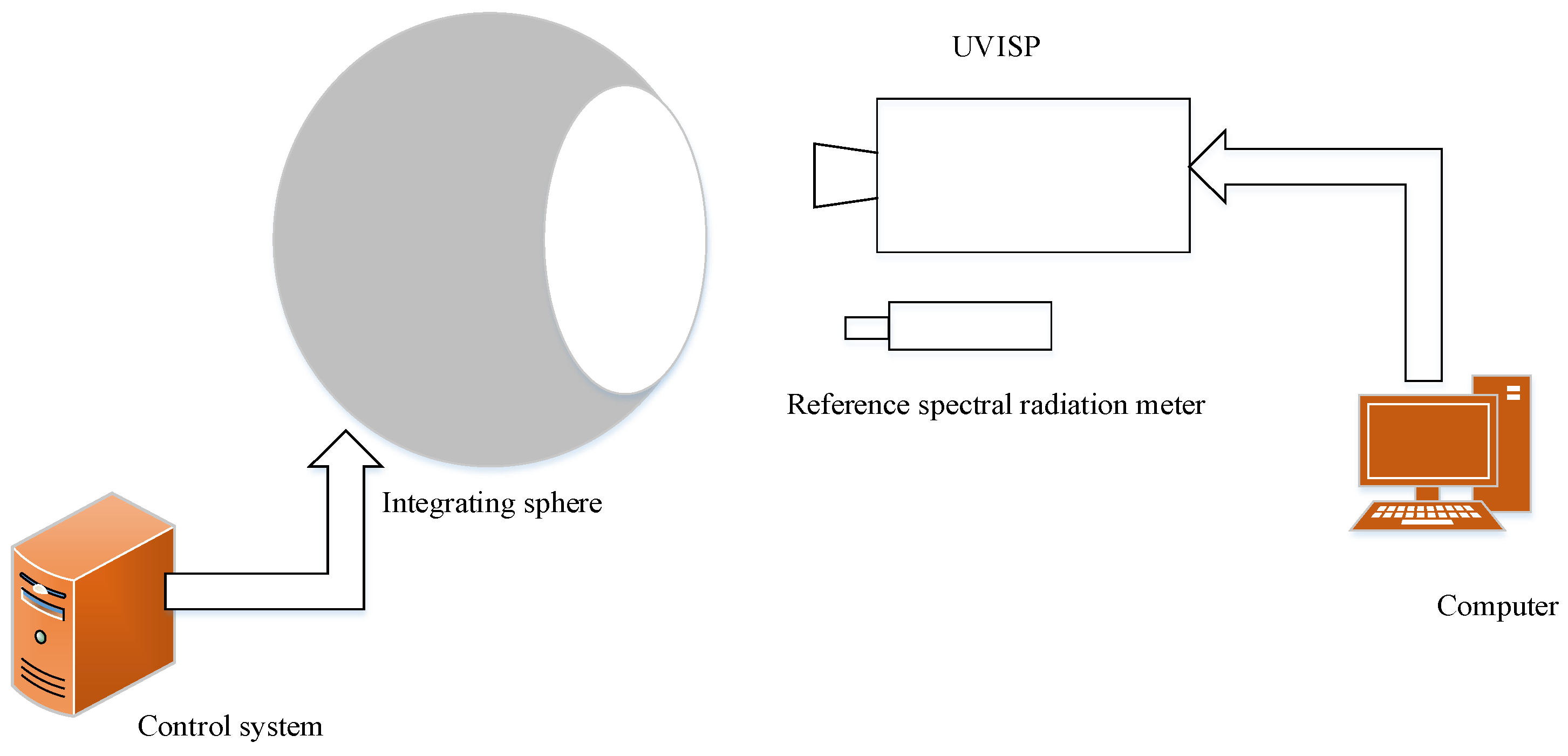
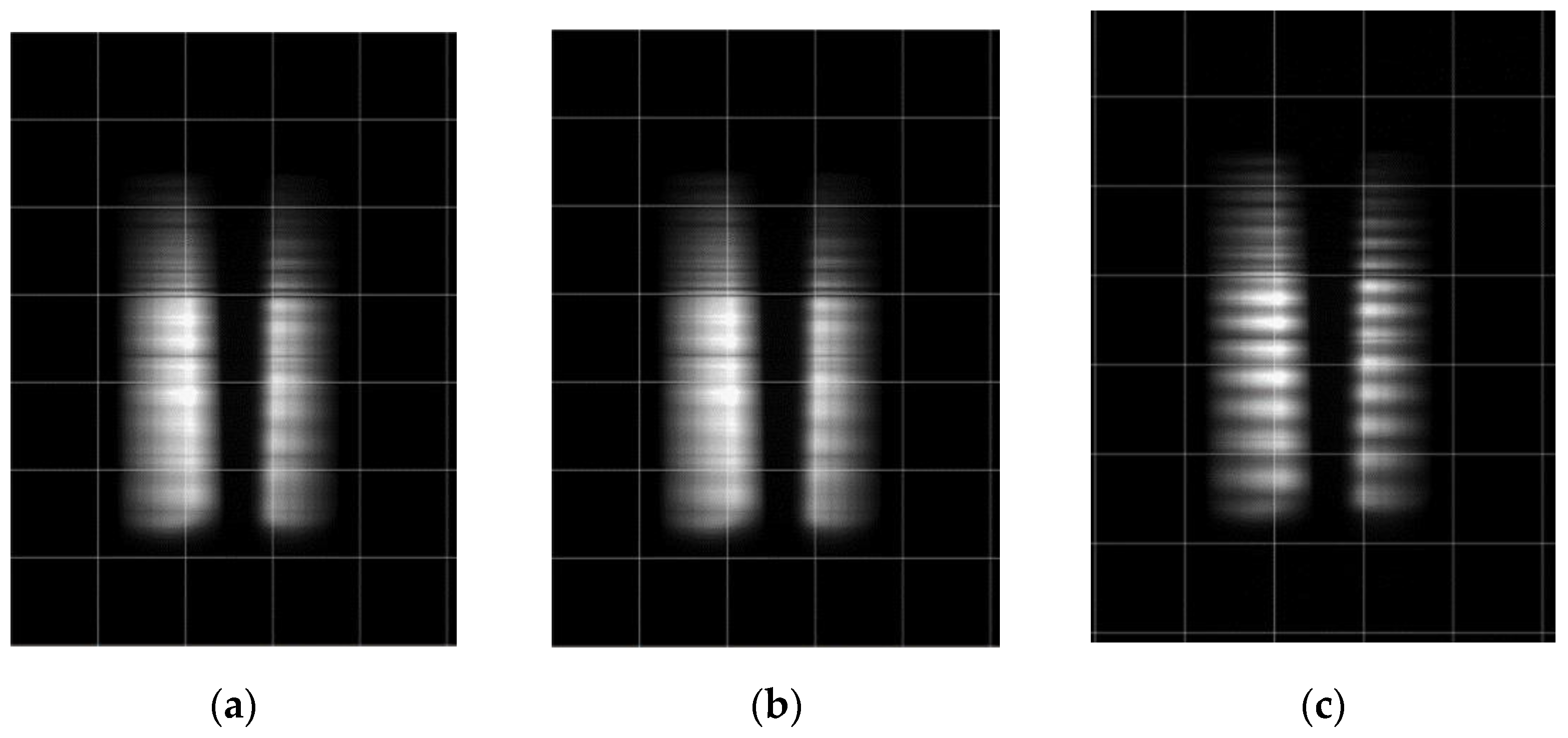
3.2. Spectral Calibration

For the spectral calibration, we chose a mercury spectral line source as the calibration light source because its characteristic spectral bandwidth is much less than the instrument spectral resolution, and the uncertainty of the wavelength for emitted light is small. The calibration source was imported into the integrating sphere to form a uniform polarization-free illumination into the instrument, which could effectively eliminate the influence of the polarization characteristics of the calibration source, and the full FOV spectrum could be calibrated at the same time.

A raw image of the integrating sphere is shown in Figure 9. First, it was necessary to extract the spectral collection with the common FOV based on geometric calibration for spectral calibration data processing. To illustrate the calibration data processing process, the spectral calibration results at a 0° FOV are given. Figure 10 shows the characteristic spectrum of the mercury spectral line source. Then, Gaussian fitting was performed for each spectrum to obtain the position of the peak in the row direction, and the pixel position was matched with the characteristic wavelength of the emission line. The results are shown in

Table 1. Wavelength–pixel matching relationship.

Wavelength (nm)	Number of Peak Pixels
	S Beam	P Beam
365.02	820.79	821.72
404.66	966.11	966.93
407.78	977.57	978.42
435.83	1080.59	1081.42
546.07	1485.68	1486.46

. Figure 11 shows the fitting results. The spectral calibration equation of the S beam is

$${\lambda }_{\mathrm{s}}=0.27225i+141.60973$$

(45)

and likewise for the P beam, it is

$${\lambda }_{\mathrm{p}}=0.2723i+141.32763$$

(46)

where ${\lambda }_{\mathrm{s}}$, ${\lambda }_{\mathrm{p}}$ denote the wavelength, and $i$ is the row index of the detector. The observation bands of the S beam and P beam covered 332.18–549.98 nm and 331.94–549.78 nm, respectively, thus meeting the needs. Then, the wavelengths were assigned to all spectral indices, and this procedure was performed for all FOVs.

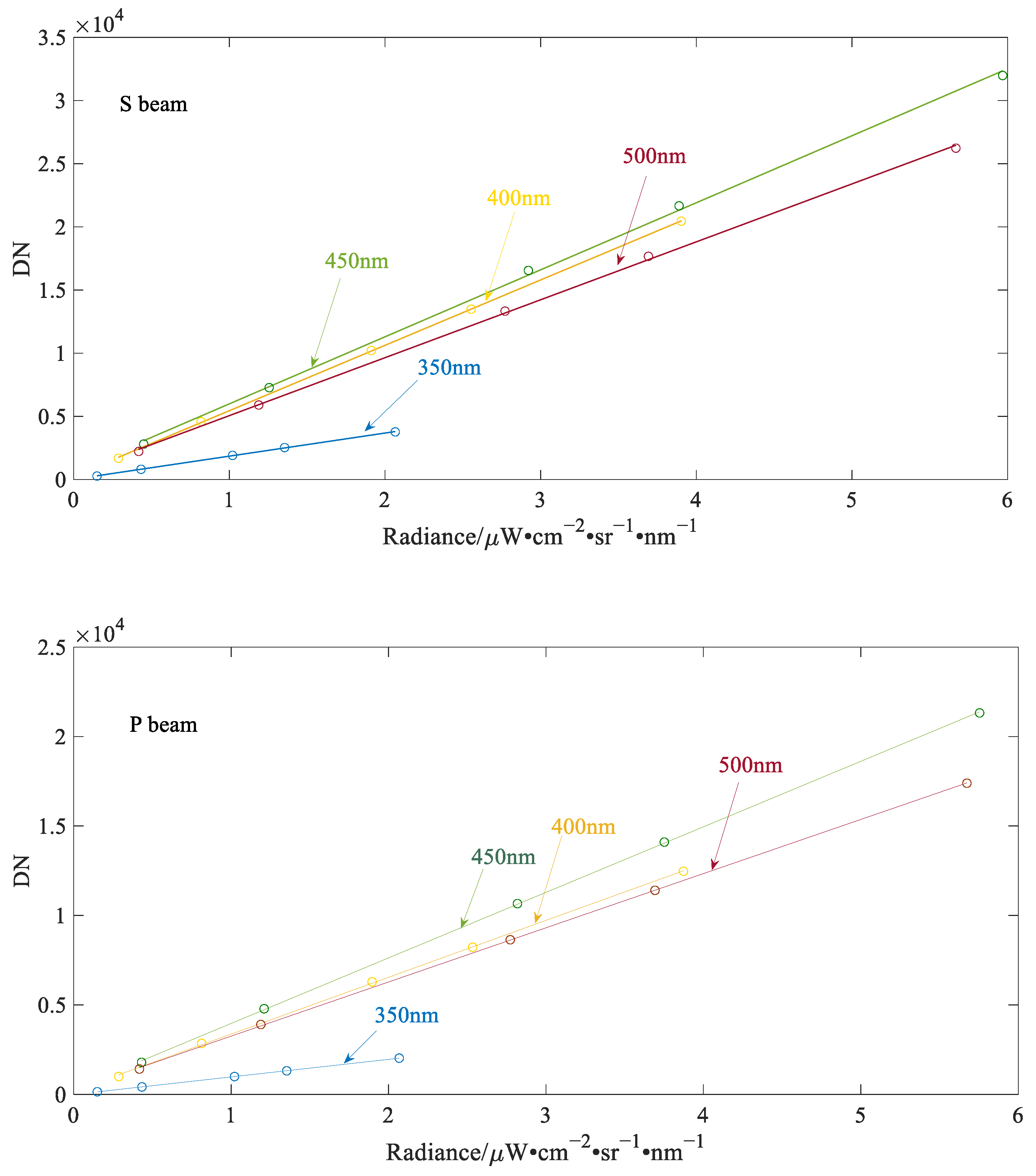
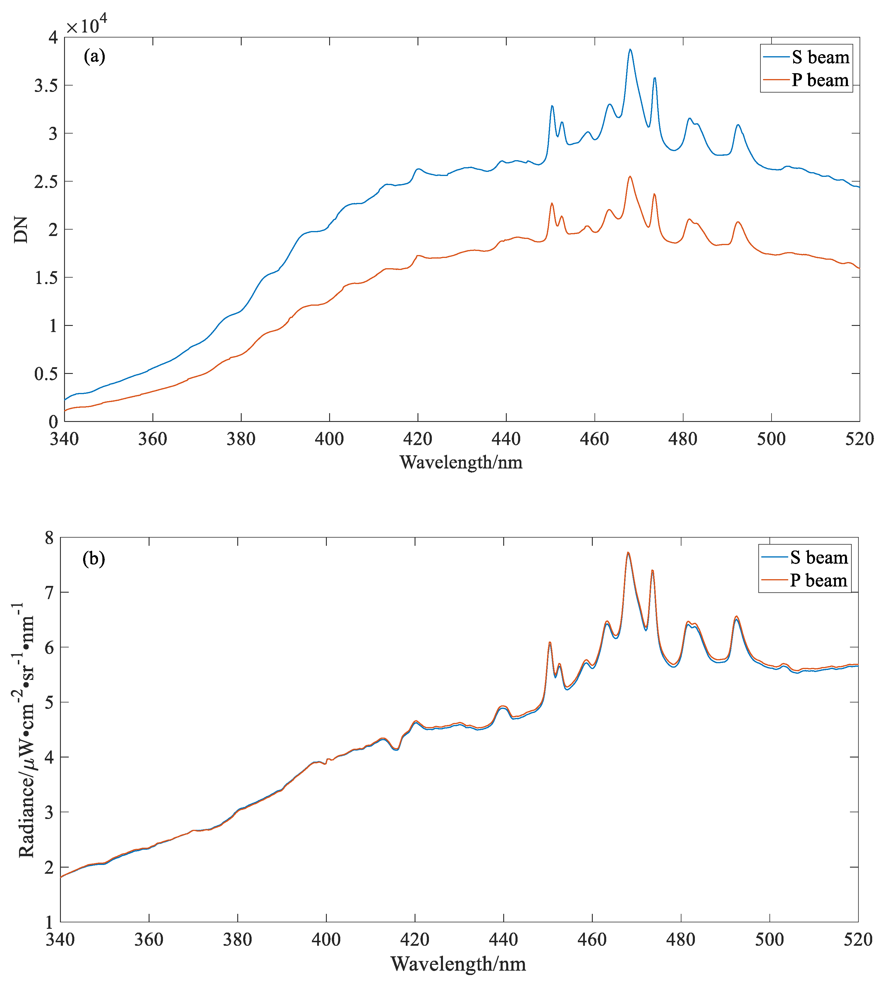
3.3. Radiometric Calibration

A schematic diagram of the radiometric calibration system is shown in Figure 12. The lamp of the integrating sphere was an LC8 ultraviolet light source. We could adjust the aperture opening size of the LC8 light source to control the output energy levels. Therefore, the output radiance of the integrating sphere had a large dynamic range, and the uniformity and stability of the output light of the integrating sphere after optimization design exceeded 98%. During the experiment, the UVISP and the reference spectral radiation meter were placed at the exit of the integrating sphere. The spectral radiance of the emitted light was measured by the reference spectral radiation meter. In this paper, the central FOV of the UVISP with an integration time of 700 ms was used as an example to give the calibration results. When the diaphragm openings in the LC8 light source were set to 4%, 12%, 29%, 39%, and 60% of the fully open state, the linear fitting results of selected bands within the spectral range are shown in Figure 13. We can see that the fitting line coincides perfectly with the measured data, indicating good linearity of the instrument’s response.

As a verification for radiometric calibration, the diaphragm opening of the LC8 light source was adjusted to 50%, and the spectrum of emitted light from the integrating sphere was recorded by the instrument and a reference spectral radiation meter. Then, the radiometric calibration coefficients were used to calculate the radiance of the S beam and P beam and compared with the measured values of the standard spectral radiance meter. Figure 14 demonstrates the comparison between the S beam and P beam. Figure 14a shows the DN values of the S beam and P beam. The spectral responsivity varies obviously for the S beam and P beam, while the yellow and blue curves in Figure 14b almost overlap each other, which indicates that the nonuniformity of the measured data was corrected effectively. In Figure 15, the line label “S + P” denotes the sum of the spectral radiance of the S beam and P beam. Comparing the measured radiance of UVISP and the reference spectral radiation meter, the differences between the two were within 2%, indicating the correctness of the radiometric calibration method.

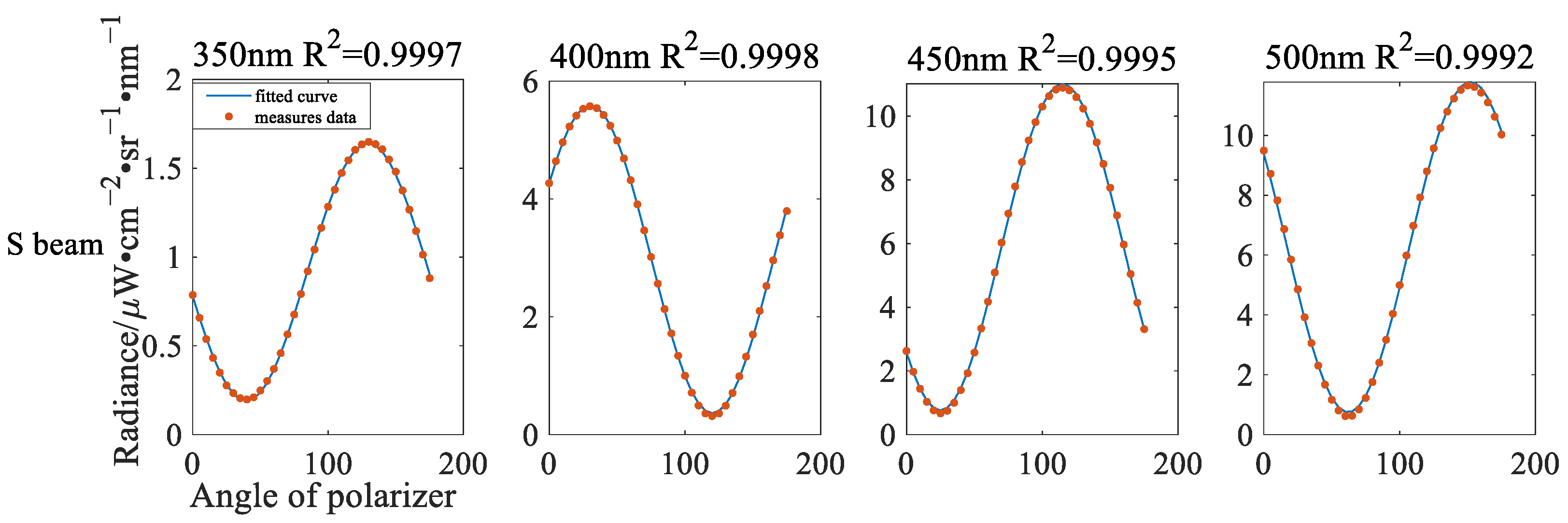
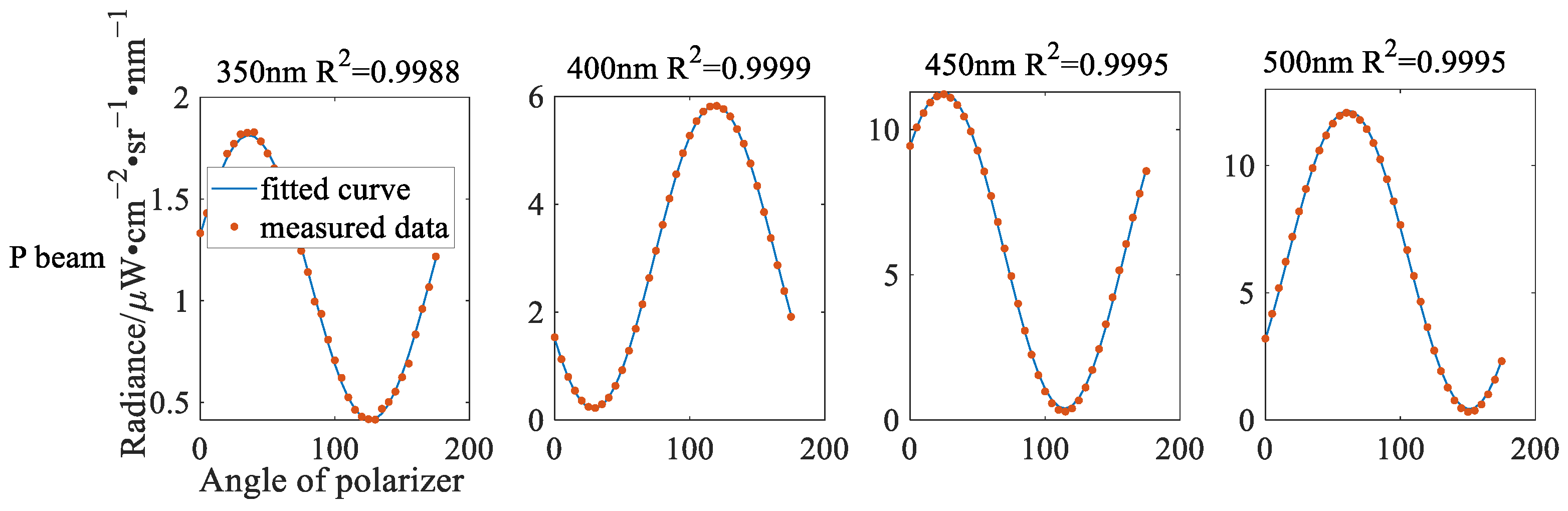
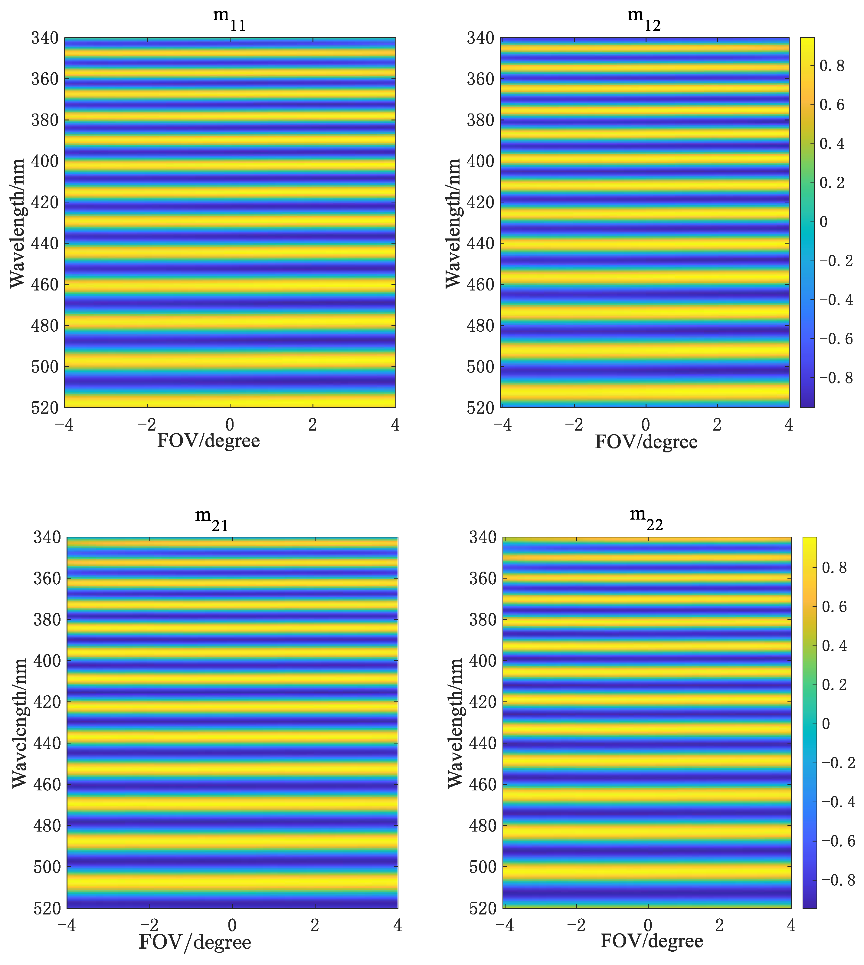
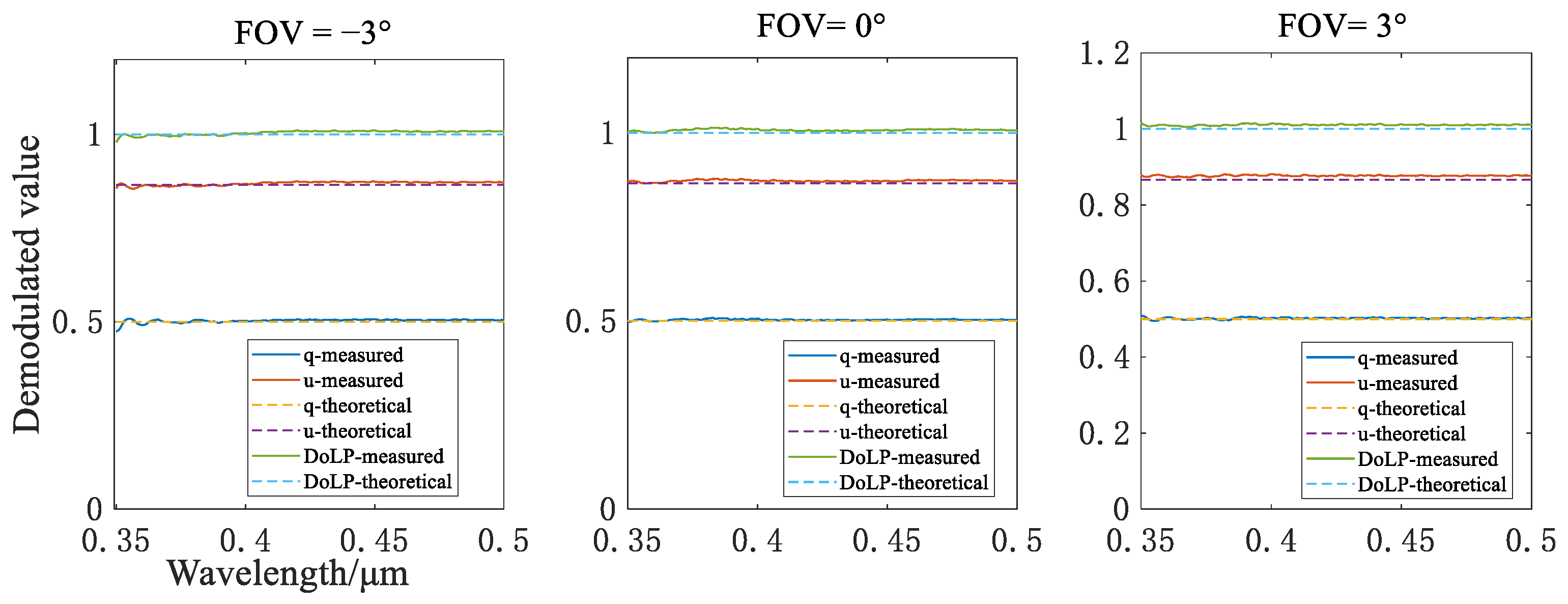
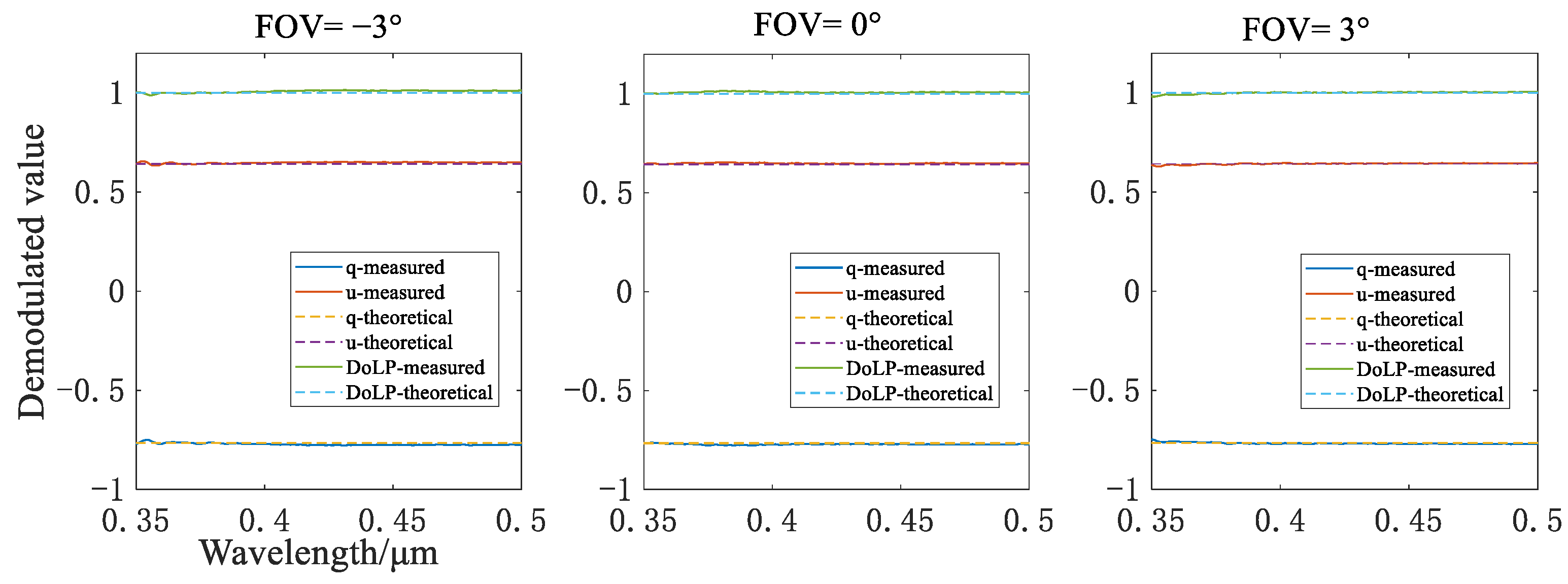
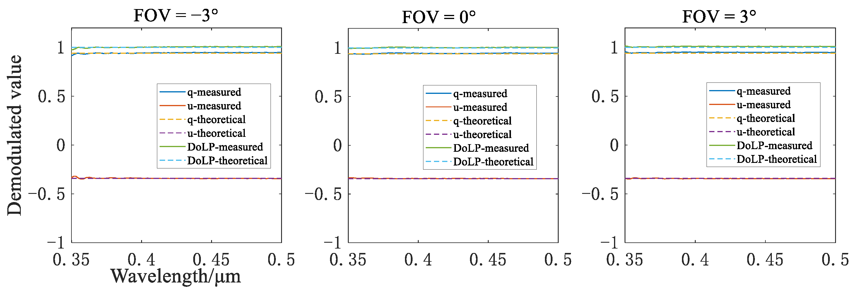
3.4. Polarimetric Calibration

The polarimetric calibration experimental system of the UVISP is shown in Figure 16, which is composed of an LC8 integrating sphere and a reference polarizer. The polarizer is a GPM-150-UNC from the Meadowlark Optics Company. Its working wavelength range is 300–2700 nm, and the extinction ratio is better than ${10}^4$ in the effective band of the instrument. The uniform incident light generated by the integrating sphere passes through the reference linear polarizer with a known orientation, and then the linearly polarized light with a fixed AoLP is received by the instrument. The polarizer rotates from 0° to 175° according to a 5° interval, and 36 kinds of completely linearly polarized light with different angles are recorded by the instrument.

Figure 17 shows an example of the fitting results and $R^2$ values at different wavelengths for one FOV of the UVISP. We can see that the $R^2$ values were all greater than 0.99, confirming that the calibration model was correct and effective. This process was performed for all wavelengths and FOVs, and the polarimetric coefficients are shown Figure 18, where the horizontal axis represents the spatial positions of different view angles, and the vertical axis represents the wavelength. Since the modulation was performed in the spectral domain, we can see that the modulation frequency was higher for shorter wavelengths. Figure 19 shows the derived polarimetric coefficients for a certain FOV. Due to the different frequencies and the imperfect spectral resolution of the spectrometer, the convolution of the spectral spread function and modulated spectrum reduced the modulation contrast, and the degree of contrast reduction was more serious for shorter wavelengths. In Figure 19, it is obvious that the modulation contrasts of the S beam and P beam are not the same. This phenomenon can be explained by the different spectral resolutions of the S beam and P beam described in Section 2.1. In addition, stray light can also influence the different modulation contrasts of the S beam and P beam because it has the same effect as a dark signal. Therefore, when imaging with a UVISP, the FOV should be filled as much as possible to remain consistent with the calibration state, in which the effect of stray light can be largely compensated by calibration coefficients.

An experiment was conducted to verify the correctness of the demodulation and polarimetric calibration method. The setup was the same as that in Figure 16, consisting of an LC8 integrating sphere and a polarizer. A rotating polarizer could produce linearly polarized light with arbitrary AoLPs. The demodulation process was performed using the following steps: (1) extracting the modulated spectrum of a certain FOV of the S beam and P beam and spectral matching, which are conducted at the same time, (2) using the radiometric calibration coefficients to correct the response differences of the S beam and P beam, and (3) applying the demodulation method presented in Section 2.3 to reconstruct the Stokes parameters.

Figure 20 demonstrates the demodulated results at input linear polarization states of 30° with normalized Stokes parameters of $\left[q=0.5,u=0.87\right]$. The spectral range of the demodulated results was within 350 to 500 nm. Figure 21 shows the reconstructed results at input linear polarization states of 70° with known normalized Stokes parameters of $\left[q=-0.77,u=0.64\right]$ over 350 to 500 nm. Additionally, Figure 22 provides the polarimetric results at input linear polarization states of 170° with normalized Stokes parameters of $\left[q=0.94,u=-0.34\right]$ at the same spectral range. It can be seen in Figure 20, Figure 21 and Figure 22 that the curves of normalized Stokes parameters for the arbitrarily selected FOVs presented good agreement with the theoretical values within the demodulated band. The RMS error over the band was calculated to evaluate the accuracy of the demodulated value.

Table 2. RMS error of the demodulated value for different angles of the polarizer.

FOV (Deg.)	Polarizer Angle (Deg.)	q RMS Error (%)	u RMS Error (%)	DoLP RMS Error (%)
−3	30	0.53	0.61	0.7
	70	0.81	0.68	1
	170	0.66	0.41	0.67
0	30	0.38	0.73	0.81
	70	0.62	0.61	0.85
	170	0.49	0.22	0.47
3	30	0.3	1.1	1.1
	70	0.42	0.51	0.51
	170	0.96	0.96	0.96

provides the RMS errors of the demodulated values for different linearly polarized inputs of 30°, 70°, and 170°. The RMS errors were all within 0.011, which proves the effectiveness and correctness of the demodulation and polarimetric calibration method.

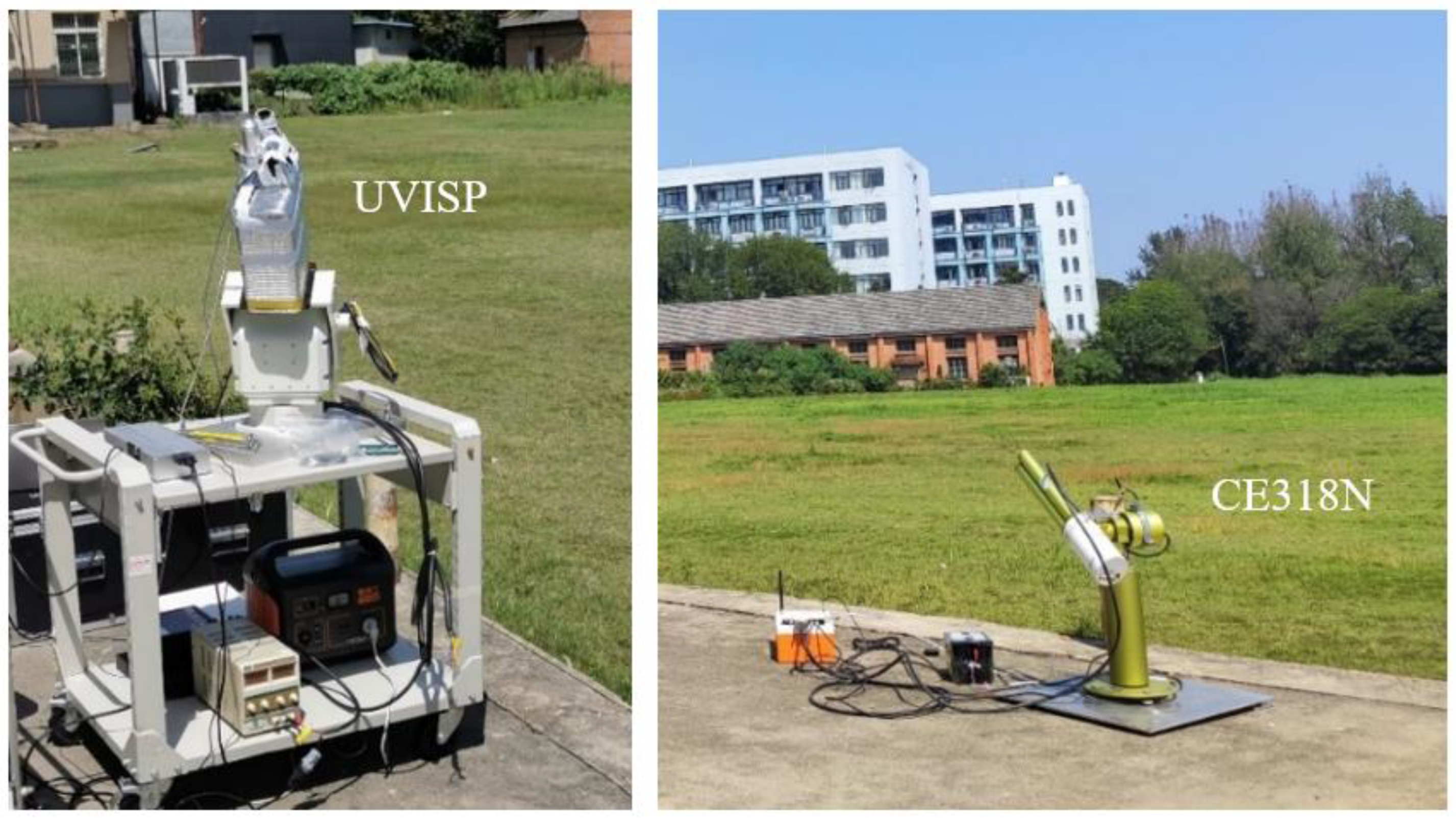
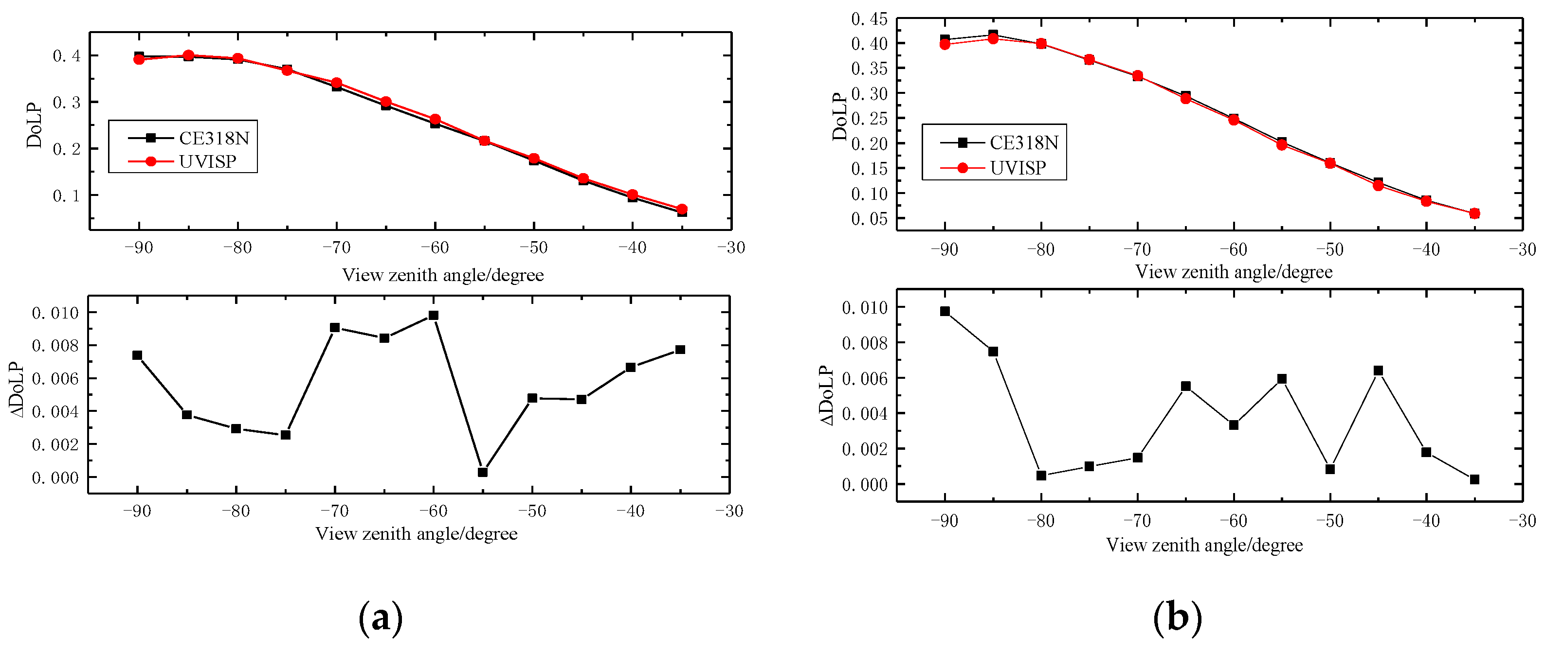
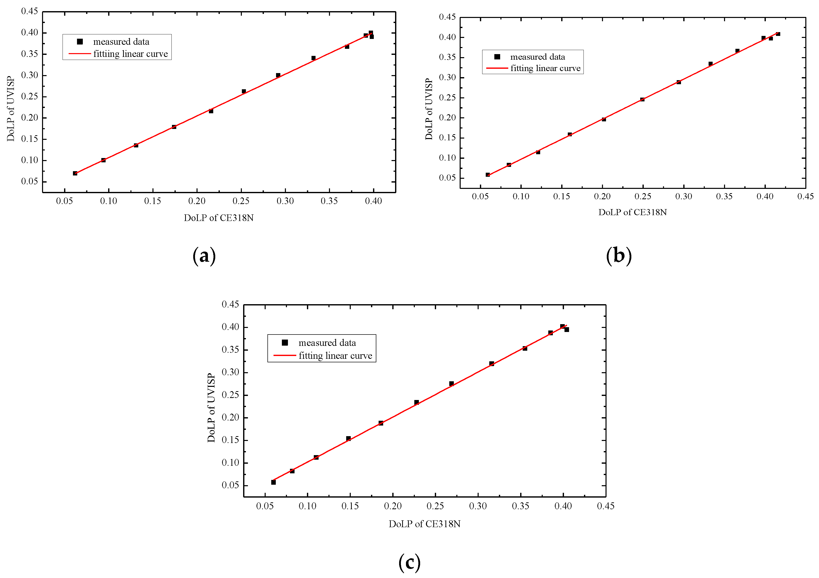
3.5. Field Measurements

We conducted an outdoor blue sky UVISP scanning experiment to further study the ability to determine the polarization properties of atmospheric aerosols. Specifically, in the outdoor environment, the UVISP obtains the polarization information of atmospheric scattering light at different positions by scanning the sky. At the same time, a CE318N photometer is used for collaborative observation. The CE318N is an instrument dedicated to ground-based polarization remote sensing detection, with nine detection bands, and its polarization measurement uncertainty is approximately 0.005 [42], which can be used as a reference standard for outdoor experimental data. The UVISP has overlapping bands with CE318N at 380, 440, and 500 nm, and we used the measured DoLPs of these bands for comparison.

To compare measurements, the UVISP and CE318N need to have similar observation geometries. The CE318N has a solar positioning function that allows scanning measurements in the principal plane of the sun. To enable the UVISP to observe the blue sky in the same solar principal plane, we designed and installed a four-quadrant solar tracker on the polarization imaging spectrometer to locate and track the sun and the tracking accuracy within 0.1°.

The experiment was performed in Hefei, China, on September 10, 2021, and the weather was clear and cloudless. The CE318N and UVISP were placed close together. Fixing the azimuth angle, both instruments set the same scanning angle step and achieved scanning in the principal plane by changing the zenith angle. The experimental site is shown in Figure 23. For this experiment, we defined the zenith angle of the sun’s position as 0°, and the scanning angle back from the sun was a negative angle. The scanning range of the zenith angle was chosen to be −35° to −90° to avoid blockage by buildings at the experimental site.

The randomly selected original images of UVISP are shown in Figure 24. Under different scanning zenith angles, the fringe contrast in the observation image is quite different. When the zenith angle is −70°, obvious modulation fringes can be seen, indicating that the solar direct light had strong polarization characteristics after scattering by atmospheric aerosol particles. Since the optical axes of the solar tracker and the UVISP were initially adjusted in the laboratory, the central FOV data of the UVISP were selected for comparison when the zenith angles of the two instruments agreed.

Figure 25 shows the demodulated DoLPs at the central FOV of the UVISP at different scanning zenith angles. The DoLP of atmospheric scattered light varied slowly with wavelength and was proportional to the zenith angle, which is consistent with the theoretical model of atmospheric scattering light, indicating the effectiveness of the instrument measurement data. Figure 26 shows the DoLP comparison results of the two instruments at the same detection band, where $\Delta DoLP=\left|DoL{P}_{\mathrm{CE}318\mathrm{N}}-DoL{P}_{\mathrm{UVISP}}\right|$ represents the absolute deviation. For the three comparison bands, the DoLPs measured by the two instruments at different zenith angles were in good agreement, and the absolute deviations were within 0.01, demonstrating the correctness of the polarization calibration method and the reliability of the measured data.

To evaluate the consistency of the measurement data of the two instruments, the CE318N data and UVISP data were linearly fitted, and the level of agreement between data was denoted by the RMS of $\Delta DoLP$. The fitting lines of the measured DoLP of the three detection bands are shown in Figure 27.

Table 3. Fitting results for overlapping bands.

Band (nm)	Slope	Intercept	RMS	${\mathit{R}}^2$
380	0.981	0.0089	0.0063	0.998
440	0.995	−0.002	0.0048	0.999
500	0.994	0.003	0.0046	0.998

presents the regression slope, intercept, linear fitting correlation, and RMS for all selected bands. From the fitting results, we can see that there were differences in the consistency levels of DoLPs between the two instruments at different bands, but the correlations were greater than 0.99, and the slopes of the fitting lines were close to 1. In addition, the RMSs of the three contrast bands were less than 0.007, indicating that the measured DoLPs of the two instruments were consistent, and that the UVISP could effectively detect the polarization characteristics of atmospheric aerosols.

4. Conclusions

The UVISP is an imaging spectropolarimeter, working in the ultraviolet to visible wavelength range, designed by AIOFM for the detection of absorbing aerosol. In this paper, an experimental scheme and data processing method for the laboratory calibration of the UVISP are presented. UVISP calibration includes geometric calibration, spectral calibration, radiometric calibration, and polarimetric calibration. In geometric calibration, we use parallel light as a calibration source and assign the FOV to each detector pixel of the UVISP. Thus, a pair of spectra for the S beam and P beam with a common FOV can be obtained. Then, spectral calibration is performed at each given spectrum of the S beam and P beam for a particular FOV, and the spectral matching method is also presented. The response uniformity of the instrument is well corrected by radiometric calibration, and the function between the output DN and spectral radiance is established using the least-squares approach. A polarimetric calibration method is proposed to improve the accuracy of polarimetric measurements. According to the radiometric model of the instrument, we derive the polarimetric calibration coefficients by measuring the incident light with different polarization states. These polarimetric coefficients include the modulation carrier and all polarization errors, such as alignment and retardance errors, modulation amplitude degradation, and other non-ideal effects of the spectral modulation module. In the polarimetric validation experiment, the RMS errors of the demodulated value for the three linear polarization states are all within 0.011, demonstrating the efficiency and accuracy of the proposed calibration method. The results of the field measurements show that the measured DoLPs of the UVISP and CE318N are in good agreement, which proves the capability to detect the polarization characteristics of atmospheric aerosols. In the future, UVISP will be used to observe atmospheric aerosols in different regions and seasons, and in the meantime, inversion algorithms based on hyperspectral polarization radiation data of UVISP will be developed to provide more accurate information on the physical properties of absorbing aerosols.

References

1. Tyo, J.S.; Goldstein, D.L.; Chenault, D.B.; Shaw, J.A. Review of passive imaging polarimetry for remote sensing applications. Appl. Opt. 2006, 45, 5453–5469. [Google Scholar] [CrossRef] [PubMed]
2. Van Harten, G.; de Boer, J.; Rietjens, J.H.H.; Di Noia, A.; Snik, F.; Volten, H.; Smit, J.M.; Hasekamp, O.P.; Henzing, J.S.; Keller, C.U. Atmospheric aerosol characterization with a ground-based SPEX spectropolarimetric instrument. Atmos. Meas. Tech. 2014, 7, 4341–4351. [Google Scholar] [CrossRef]
3. Meng, X.; Li, J.; Liu, D.; Zhu, R. Fourier transform imaging spectropolarimeter using simultaneous polarization modulation. Opt. Lett. 2013, 38, 778–780. [Google Scholar] [CrossRef]
4. Mu, T.; Pacheco, S.; Chen, Z.; Zhang, C.; Liang, R. Snapshot linear-Stokes imaging spectropolarimeter using division-of-focal-plane polarimetry and integral field spectroscopy. Sci. Rep. 2017, 7, 42115. [Google Scholar] [CrossRef]
5. Diner, D.; Chipman, R.; Beaudry, N.; Cairns, B.; Foo, L.; Macenka, S.; Cunningham, T.; Seshadri, S.; Keller, C. An Integrated Multiangle, Multispectral, and Polarimetric Imaging Concept for Aerosol Remote Sensing from Space; SPIE: Bellingham, WA, USA, 2005; Volume 5659. [Google Scholar]
6. Pust, N.J.; Shaw, J.A. Wavelength dependence of the degree of polarization in cloud-free skies: Simulations of real environments. Opt. Express 2012, 20, 15559–15568. [Google Scholar] [CrossRef] [PubMed]
7. Okabe, H.; Hayakawa, M.; Naito, H.; Taniguchi, A.; Oka, K. Spectroscopic polarimetry using channeled spectroscopic polarization state generator (CSPSG). Opt. Express 2007, 15, 3093–3109. [Google Scholar] [CrossRef]
8. Okabe, H.; Matoba, K.; Hayakawa, M.; Taniguchi, A.; Oka, K.; Naito, H.; Nakatsuka, N. New Configuration of Channeled Spectropolarimeter for Snapshot Polarimetric Measurement of Materials; SPIE: Bellingham, WA, USA, 2005; Volume 5878. [Google Scholar]
9. Zhao, Y.; Zhang, L.; Pan, Q. Spectropolarimetric imaging for pathological analysis of skin. Appl. Opt. 2009, 48, D236–D246. [Google Scholar] [CrossRef]
10. Rivet, S.; Dubreuil, M.; Bradu, A.; Le Grand, Y. Fast spectrally encoded Mueller optical scanning microscopy. Sci. Rep. 2019, 9, 3972. [Google Scholar] [CrossRef]
11. Nordsieck, K.H. A Simple Polarimetric System for the Lick Observatory Image-Tube Scanner. Publ. Astron. Soc. Pac. 1974, 86, 324. [Google Scholar] [CrossRef]
12. Oka, K.; Kato, T. Spectroscopic polarimetry with a channeled spectrum. Opt. Lett. 1999, 24, 1475–1477. [Google Scholar] [CrossRef]
13. Iannarilli, F.; Jones, S.; Scott, H.; Kebabian, P. Polarimetric-Spectral Intensity Modulation (P-SIM): Enabling Simultaneous Hyperspectral and Polarimetric Imaging; SPIE: Bellingham, WA, USA, 1999; Volume 3698. [Google Scholar]
14. Li, J.; Gao, B.; Qi, C.; Zhu, J.; Hou, X. Tests of a compact static Fourier-transform imaging spectropolarimeter. Opt. Express 2014, 22, 13014–13021. [Google Scholar] [CrossRef] [PubMed]
15. Quan, N.; Zhang, C.; Mu, T. Static Fourier transform imaging spectropolarimeter based on quarter-wave plate array. Optik 2016, 127, 9763–9774. [Google Scholar] [CrossRef]
16. LaCasse, C.F.; Craven, J.M.; Lowenstern, M.E.; Kudenov, M.W. Field deployable pushbroom hyperspectral imaging polarimeter. Opt. Eng. 2017, 56, 1. [Google Scholar] [CrossRef]
17. Jones, S.; Iannarilli, F.; Kebabian, P. Realization of quantitative-grade fieldable snapshot imaging spectropolarimeter. Opt. Express 2004, 12, 6559–6573. [Google Scholar] [CrossRef]
18. Shaw, J.A.; Hagen, N.; Tyo, J.S.; Dereniak, E.L.; Sass, D.T. Visible snapshot imaging spectro-polarimeter. In Polarization Science and Remote Sensing II; SPIE: Bellingham, WA, USA, 2005; Volume 5888. [Google Scholar]
19. LaCasse, C.F.; Chipman, R.A.; Tyo, J.S. Band limited data reconstruction in modulated polarimeters. Opt. Express 2011, 19, 14976–14989. [Google Scholar] [CrossRef]
20. Lee, D.J.; LaCasse, C.F.; Craven, J.M. Compressed channeled spectropolarimetry. Opt. Express 2017, 25, 32041–32063. [Google Scholar] [CrossRef]
21. Kudenov, C.M.W. False signature reduction in channeled spectropolarimetry. Opt. Eng. 2010, 49, 053602. [Google Scholar]
22. Kadowaki, N.; Moon, S.G.; ter Horst, R.; Keller, C.U.; Voors, R.; Wielinga, K.; Navarro, R.; Laan, E.C.; Verlaan, A.L.; van Harten, G.; et al. SPEX: The Spectropolarimeter for Planetary Exploration. In International Conference on Space Optics—ICSO 2010; SPIE: Bellingham, WA, USA, 2010; Volume 105651C. [Google Scholar] [CrossRef]
23. Meynart, R.; Voors, R.; Neeck, S.P.; Moon, S.G.; Hannemann, S.; Shimoda, H.; Rietjens, J.H.H.; van Harten, G.; Snik, F.; Smit, M.; et al. Spectropolarimeter for planetary exploration (SPEX): Performance measurements with a prototype. In Sensors, Systems, and Next-Generation Satellites XV; SPIE: Bellingham, WA, USA, 2011; Volume 8176. [Google Scholar] [CrossRef]
24. Smit, J.M.; Rietjens, J.H.H.; di Noia, A.; Hasekamp, O.P.; Laauwen, W.; Cairns, B.; van Diedenhoven, B.; Wasilewski, A.; Karafolas, N.; Sodnik, Z.; et al. In-flight validation of SPEX airborne spectro-polarimeter onboard NASA’s research aircraft ER-2. In International Conference on Space Optics—ICSO 2018; SPIE: Bellingham, WA, USA, 2019; Volume 11180. [Google Scholar] [CrossRef]
25. Rietjens, J.H.H.; Campo, J.; Chanumolu, A.; Smit, M.; Nalla, R.; Fernandez, C.V.; Dingjan, J.; van Amerongen, A.; Hasekamp, O.P.; Snik, F.; et al. Expected performance and error analysis for SPEXone, a multi-angle channeled spectropolarimeter for the NASA PACE mission. In Polarization Science and Remote Sensing IX; SPIE: Bellingham, WA, USA, 2019. [Google Scholar] [CrossRef]
26. Goldstein, D.H.; Chenault, D.B.; Wu, D.L.; Chipman, R.A.; Hart, K. Compact LWIR polarimeter for cirrus ice properties. In Polarization: Measurement, Analysis, and Remote Sensing XIII; SPIE: Bellingham, WA, USA, 2018. [Google Scholar] [CrossRef]
27. Hart, K. Linear Stokes measurement of thermal targets using compact LWIR spectropolarimeter. In Polarization: Measurement, Analysis, and Remote Sensing XIV; SPIE: Bellingham, WA, USA, 2020. [Google Scholar] [CrossRef]
28. DeLeon, C.M.; Heath, J.; Espinosa, W.R.; Wu, D.; Kupinski, M.; Snik, F.; Kupinski, M.K.; Shaw, J.A. UV linear stokes imaging of optically thin clouds. In Polarization Science and Remote Sensing X; SPIE: Bellingham, WA, USA, 2021. [Google Scholar] [CrossRef]
29. Olson, M.R.; Yuqin, W.; de Foy, B.; Li, Z.; Bergin, M.H.; Zhang, Y.; Schauer, J.J. Source attribution of black and Brown carbon near-UV light absorption in Beijing, China and the impact of regional air-mass transport. Sci. Total Environ. 2022, 807, 150871. [Google Scholar] [CrossRef]
30. Sabatke, D.S.; Locke, A.M.; Dereniak, E.L.; McMillan, R.W. Linear operator theory of channeled spectropolarimetry. J. Opt. Soc. Am. A 2005, 22, 1567–1576. [Google Scholar] [CrossRef]
31. Sabatke, D.S.; Locke, A.M.; Dereniak, E.L.; McMillan, R.W. Linear calibration and reconstruction techniques for channeled spectropolarimetry. Opt. Express 2003, 11, 2940–2952. [Google Scholar] [CrossRef]
32. Ju, X.; Yang, B.; Yan, C.; Zhang, J.; Xing, W. Easily implemented approach for the calibration of alignment and retardation errors in a channeled spectropolarimeter. Appl. Opt. 2018, 57, 8600–8613. [Google Scholar] [CrossRef] [PubMed]
33. Mu, T.; Zhang, C.; Jia, C.; Ren, W.; Zhang, L.; Li, Q. Alignment and retardance errors, and compensation of a channeled spectropolarimeter. Opt. Commun. 2013, 294, 88–95. [Google Scholar] [CrossRef]
34. Yang, B.; Zhang, J.; Yan, C.; Ju, X. Methods of polarimetric calibration and reconstruction for a fieldable channeled dispersive imaging spectropolarimeter. Appl. Opt. 2017, 56, 8477. [Google Scholar] [CrossRef] [PubMed]
35. Xing, W.; Ju, X.; Yan, C.; Yang, B.; Zhang, J. Self-correction of alignment errors and retardations for a channeled spectropolarimeter. Appl. Opt. 2018, 57, 7857–7864. [Google Scholar] [CrossRef]
36. Li, Q.; Zhang, C.; Yan, T.; Wei, Y. Polarization state demodulation of channeled imaging spectropolarimeter by phase rearrangement calibration method. Opt. Commun. 2016, 379, 54–63. [Google Scholar] [CrossRef]
37. Van Harten, G.; Snik, F.; Rietjens, J.H.H.; Smit, J.M.; de Boer, J.; Diamantopoulou, R.; Hasekamp, O.P.; Stam, D.M.; Keller, C.U.; Laan, E.C.; et al. Prototyping for the Spectropolarimeter for Planetary EXploration (SPEX): Calibration and sky measurements. In Polarization Science and Remote Sensing V; SPIE: Bellingham, WA, USA, 2011; Volume 8160. [Google Scholar] [CrossRef]
38. Smit, J.M.; Rietjens, J.H.H.; van Harten, G.; Di Noia, A.; Laauwen, W.; Rheingans, B.E.; Diner, D.J.; Cairns, B.; Wasilewski, A.; Knobelspiesse, K.D.; et al. SPEX airborne spectropolarimeter calibration and performance. Appl. Opt. 2019, 58, 5695–5719. [Google Scholar] [CrossRef]
39. Hart, K.; Kupinski, M.; Wu, D.; Chipman, R. First results from an uncooled LWIR polarimeter for cubesat deployment. Opt. Eng. 2020, 59, 075103. [Google Scholar] [CrossRef]
40. Xing, W.; Ju, X.; Bo, J.; Yan, C.; Yang, B.; Xu, S.; Zhang, J. Polarization Radiometric Calibration in Laboratory for a Channeled Spectropolarimeter. Appl. Sci. 2020, 10, 8295. [Google Scholar] [CrossRef]
41. Snik, F.; Karalidi, T.; Keller, C.U. Spectral modulation for full linear polarimetry. Appl. Opt. 2009, 48, 1337–1346. [Google Scholar] [CrossRef]
42. Dubovik, O.; Smirnov, A.; Holben, B.N.; King, M.D.; Kaufman, Y.J.; Eck, T.F.; Slutsker, I. Accuracy assessments of aerosol optical properties retrieved from Aerosol Robotic Network (AERONET) Sun and sky radiance measurements. J. Geophys. Res. Atmos. 2000, 105, 9791–9806. [Google Scholar] [CrossRef]
Figure 1. (a) Optical layout of UVISP. (b) Schematic representation of light rays through the UVISP optic system. The components are: 1. SMM, 1.1. QWR, 1.2. MOR, 1.3. WP, 2. focusing lens, 3. Spectrometer system, 3.11. slit, 3.12. diffraction grating, 3.2. detector component, 3.13, 3.14, 3.15. reflector set. The light is incident from the left; passes through the QWR, MOR, and WP in turn; is focused on the slit by the lens; and finally enters the dispersion system. In fact, both the WP beam splitting direction and the slit direction are perpendicular to the paper surface. (c) Distribution of modulated spectra on the detector when the incident light is fully linearly polarized.
Remotesensing 14 03898 g001aRemotesensing 14 03898 g001b
Figure 2. Diagram of the simplified optical system.
Remotesensing 14 03898 g002
Figure 3. Geometric calibration site.
Remotesensing 14 03898 g003
Figure 4. Original image at 4° FOV of UVISP.
Remotesensing 14 03898 g004
Figure 5. Results of Gaussian fitting of the normalized data.
Remotesensing 14 03898 g005
Figure 6. Collection of pixels from incident parallel light at various angles.
Remotesensing 14 03898 g006
Figure 7. (ah) Linear regression results for the S beam and P beam.
Remotesensing 14 03898 g007aRemotesensing 14 03898 g007b
Figure 8. Difference between the model theoretical view angles and the actual view angles in different row pixels.
Remotesensing 14 03898 g008
Figure 9. Raw image of integrating sphere.
Remotesensing 14 03898 g009
Figure 10. The characteristic spectrum of the mercury spectral line source at 0° FOV of UVISP.
Remotesensing 14 03898 g010
Figure 11. Fitting results of the relationship between pixel and wavelength.
Remotesensing 14 03898 g011
Figure 12. Schematic diagram of the radiometric calibration system.
Remotesensing 14 03898 g012
Figure 13. Fitting results of UVISP for selected bands.
Remotesensing 14 03898 g013
Figure 14. Comparison of the S beam and P beam before and after radiometric calibration: (a) the DN value of the S beam and P beam; (b) the spectral radiance of the S beam and P beam.
Remotesensing 14 03898 g014
Figure 15. Comparison of measured radiance for “S + P” and the spectral radiation meter.
Remotesensing 14 03898 g015
Figure 16. The polarimetric calibration experimental system of the UVISP.
Remotesensing 14 03898 g016
Figure 17. Single selected wavelength fit for the S beam and P beam.
Remotesensing 14 03898 g017aRemotesensing 14 03898 g017b
Figure 18. Derived polarimetric coefficients.
Remotesensing 14 03898 g018
Figure 19. The polarimetric coefficients of a selected field of view of UVISP.
Remotesensing 14 03898 g019
Figure 20. Demodulated value for input polarization states at 30°.
Remotesensing 14 03898 g020
Figure 21. Demodulated value for input polarization states at 70°.
Remotesensing 14 03898 g021
Figure 22. Demodulated value for input polarization states at 170°.
Remotesensing 14 03898 g022
Figure 23. The outdoor experimental site.
Remotesensing 14 03898 g023
Figure 24. Raw images at selected zenith angles: (a) zenith angle −40°; (b) zenith angle −50°; (c) zenith angle −70°.
Remotesensing 14 03898 g024
Figure 25. The measured DoLPs of UVISP for different zenith angles.
Remotesensing 14 03898 g025
Figure 26. Comparison of CE318N and UVISP at overlapping bands: (a) 380 nm; (b) 440 nm; (c) 500 nm.
Remotesensing 14 03898 g026aRemotesensing 14 03898 g026b
Figure 27. DoLP measured by CE318N and UVISP at spectral bands at 380 nm, 440 nm, and 500 nm, and the fitting result of the three detected bands: (a) 380 nm; (b) 440 nm; (c) 500 nm.
Remotesensing 14 03898 g027