Increasing Atmospheric Aridity Moderates the Accelerated Rate of Vegetation Green-Up Induced by Rising CO₂ and Warming

Abstract

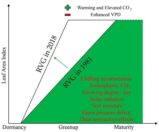
The rate of vegetation green-up (RVG) indicates the ability of vegetation to respond to changes in climatic conditions. Understanding long-term RVG trends can clarify the changes in how quickly the vegetation grows from dormancy to maturity with time. However, how RVG trends respond to environmental variables and variable interactions remains unknown. We examined the long-term RVG trends (1981–2018) over the northern extratropics and determined the influence of environment variables and interactions between variables on the RVG trends based on the Global Land Surface Satellite leaf area index and a multivariable regression considering interactions between variables (MRCI). Our results showed a persistent increase in RVG at 0.020% (8-day)⁻¹ year⁻¹ over the entire region. Except for shrublands (−0.032% (8-day)⁻¹ year⁻¹), RVG trends increased significantly, particularly in woody savannas (0.095% (8-day)⁻¹ year⁻¹) and mixed forests (0.076% (8-day)⁻¹ year⁻¹). The relative importance of interactive effects (RI_IAE) to the RVG trends is roughly 30%. Rising CO₂, enhanced vapor pressure deficit (VPD), and warming are the primary factors affecting the RVG trends, both at the pixel and the biome scales. The accelerated RVG is triggered by both rising CO₂ and warming but is partially offset by increased VPD. Our findings shed light on the relative contribution of variable interactions and assessed the relationship between environmental factors and RVG trends across different biomes, hence strengthening our knowledge of vegetation spring green-up in response to global change.

1. Introduction

Vegetation of the northern extratropics is shifting its seasonal growth cycles to adapt to global change [1,2,3]. Changes in vegetation phenology are considered clear signals that global changes affect terrestrial ecosystems [4,5]. Previous studies, however, had already centered on discrete phenological events such as the start of the growing season [6], the length of the growing season [7], and the peak of the growing season [8], with little attention paid to continuous phenological events such as spring green-up or autumn senescence, which reflect how quickly the vegetation can respond to changes in climatic conditions [9]. Thus, continuous phenological events should be studied to have a better understanding of how vegetation grows in the context of global change.

The rate of vegetation green-up (RVG) represents the growing velocity of plant growth over time from dormancy to maturity [2,10]. Variations in RVG influence annual carbon assimilation due to altering the growing season length [9], and consequently affect the biosphere–atmosphere exchange of energy, carbon, and water [11,12]. Previous studies suggest that several variables such as atmospheric carbon dioxide concentrations (CO₂), temperature, and water availability might affect the vegetation greening rate individually or interactively [2,13,14]. Rising CO₂ could enhance carboxylation and enhance water use efficiency [15], thus promoting foliage development and vegetation productivity [16,17]. A growing body of evidence suggests that spring phenology is extremely sensitive to temperature change [10,14,18,19,20] and that RVG acceleration is strongly linked to warming at high latitudes [2]. Although precipitation has a minimal influence on the RVG trends [2], plant water stress is largely reliant on the conditions of atmospheric aridity and soil moisture. Current research suggests that the intensification of atmospheric aridity over the past few decades has had a profound effect on ecosystems [21]. Given the influence of water on the greening rate, particularly in arid/semiarid terrestrial ecosystems [22], the function of water scarcity on leaf development must be investigated further.

During the greening of plants, it is impossible to disregard the complex interactions involving temperature, radiation, water availability, and atmospheric CO₂ concentrations [10,23,24]. For example, warming may enhance the drought risk of the ecosystem because the increasing evaporation would enhance soil water consumption and exacerbate drought conditions for plants [21]. Cook et al. [24] found that warming could reduce chilling accumulation and then accelerate spring leaf expansion because the reduced chilling accumulation could delay the date of leaf unfolding. Generally, the effects of elevated atmospheric CO₂ concentrations on plant development are regulated by temperature [25], nutrient limitation, and water availability [26,27]. The CO₂ fertilization effect requires an ample level of water and nutrients, i.e., an absence of drought and nutrient stress effects. In other words, the benefits of the CO₂ fertilization effect could be reduced in the case of water scarcity and a lack of soil nutrients. While the mechanics of these interactions are closely connected to plant phenology and growth, the influences of interactions on vegetation greening rate remain scarce. Moreover, there are biome-specific shifts in vegetation phenology [28], meaning that variations in leaf development can be affected by the makeup of the various forest types [14]. In contrast, at the biome level, the effects of multiple environmental factors and their interactions on the trends of leaf development are still not well understood, and a thorough understanding of the RVG trends and environmental factors is essential.

In this study we firstly analyzed the long-term RVG trends (1981–2018) across the northern extratropics and across different biomes. Secondly, we assessed the relative importance of interactive effects at the pixel and biome scales employing the multivariable linear regression considering interactions between variables. Finally, we examined the dominant factors driving the RVG trends at the pixel scale over the northern extratropics, as well as factor attribution across the different biomes. The purpose of this research was to determine the influence of each variable and their interactions on the RVG trends, and to gain a better understanding of spring vegetation green-up in response to climate change.

2. Materials and Methods

2.1. The Global Land Surface Satellite Leaf Area Index (GLASS LAI) and Land-Cover Classification

The Global Land Surface Satellite leaf area index (GLASS LAI version 5), which is produced by general regression neural networks based on AVHRR (http://glass.umd.edu/, accessed on 6 July 2021), covers the world at a 0.05° spatial resolution and an 8-day time interval from 1981–2018 [29]. We chose GLASS LAI in this work because it exhibits superior quality and accuracy over other long-term LAI products [30,31]. In our research, we used the International Geosphere-Biosphere Programme (IGBP) global land-cover classification MCD12C1 product (https://search.earthdata.nasa.gov/, accessed on 8 July 2021), which has a spatial resolution of 0.05° for the entire globe from 2001 to 2018 [32]. Given the mismatch between time periods of the MCD12C1 dataset (2001 to 2018) and the study period (1981–2018), the authors primarily focused on pixels that did not suffer changes in deciduous vegetation types. Finally, the land cover data were divided into seven classes, including deciduous needleleaf forests (DNF), deciduous broadleaf forests (DBF), mixed forests (MIF), shrublands (SHL), woody savannas (WSN), savannas (SVN), and grasslands (GRL).

2.2. Environmental Variables Data

Fundamental climatic variables (air temperature at 2 m, relative humidity, volumetric soil moisture, and solar radiation at the surface) were obtained from the Copernicus Climate Data Store [33], and the CO₂ concentrations dataset was retrieved from the atmospheric CO₂ field simulations (sEXTocNEET_v4.3: http://www.bgc-jena.mpg.de/CarboScope, accessed on 10 July 2021) [34]. Next, the nearest-neighbor method was used to interpolate the datasets to the 0.05° spatial resolution. We calculated the following six environmental variables for each pixel and each year from 1981–2018: chilling accumulation (CA), CO₂, growing degree-day (GDD), solar radiation (RD), soil moisture (SM), and VPD. Calculations were completed using Equations (1)–(6) as follows:

$${\mathrm{CA}}_{\mathrm{RVG}}={\displaystyle \sum }_{\mathrm{Jan}1\mathrm{st}}^{{\mathrm{SOS}}_{\mathrm{clim}}}\left\{\begin{array}{c}0 \mathrm{for} \mathrm{T}\left(\mathrm{t}\right)<0 ℃\\ 1 \mathrm{for} 0 ℃\le \mathrm{T}\left(\mathrm{t}\right)\le 5 ℃ \\ 0 \mathrm{for} \mathrm{T}\left(\mathrm{t}\right)>5 ℃\end{array}\right.$$

(1)

$${\mathrm{CO}}_{2_{\mathrm{RVG}}}=\frac{{{\displaystyle \sum }}_{\mathrm{Jan}1\mathrm{st}}^{{\mathrm{SOS}}_{\mathrm{clim}}}\mathrm{C}\left(\mathrm{t}\right)}{{\mathrm{SOS}}_{\mathrm{clim}}-\mathrm{Jan}1\mathrm{st}}$$

(2)

$${\mathrm{GDD}}_{\mathrm{RVG}}={\displaystyle \sum }_{\mathrm{Jan}1\mathrm{st}}^{{\mathrm{SOS}}_{\mathrm{clim}}}\left\{\begin{array}{c}0 \mathrm{for} \mathrm{T}\left(\mathrm{t}\right)<0 ℃\\ \mathrm{T}\left(\mathrm{t}\right)-0 ℃ \mathrm{for} \mathrm{T}\left(\mathrm{t}\right)\ge 0 ℃\end{array}\right.$$

(3)

$${\mathrm{RD}}_{\mathrm{RVG}}={\displaystyle \sum }_{{\mathrm{SOS}}_{\mathrm{clim}}-15}^{{\mathrm{SOS}}_{\mathrm{clim}}+15}\mathrm{R}\left(\mathrm{t}\right)$$

(4)

$${\mathrm{SM}}_{\mathrm{RVG}}=\frac{{{\displaystyle \sum }}_{\mathrm{Jan}1\mathrm{st}}^{{\mathrm{SOS}}_{\mathrm{clim}}}\mathrm{M}\left(\mathrm{t}\right)}{{\mathrm{SOS}}_{\mathrm{clim}}-\mathrm{Jan}1\mathrm{st}}$$

(5)

$${\mathrm{VPD}}_{\mathrm{RVG}}=\frac{{{\displaystyle \sum }}_{\mathrm{Jan}1\mathrm{st}}^{{\mathrm{SOS}}_{\mathrm{clim}}}\mathrm{V}\left(\mathrm{t}\right)}{{\mathrm{SOS}}_{\mathrm{clim}}-\mathrm{Jan}1\mathrm{st}}$$

(6)

where T(t), C(t), R(t), M(t), and V(t) represent daily temperature at 2 m (°C), atmosphere CO₂ concentrations (ppm), surface solar radiation (J m⁻²), soil moisture (m³ m⁻³), and vapor pressure deficit (hpa), respectively. SOS_clim indicates the climatological start of the growing season (SOS) averaged during 1981–2018 for each pixel. CA is the number of days when the daily temperature is >0 and <5 °C from the first day of a year to SOS_clim. The GDD is defined as the accumulated temperature (>0 °C) from the first day of a year to SOS_clim. RD measures the intensity of surface solar radiation absorbed for 31 days around SOS_clim, when high light intensity can accelerate green-up processes [35]. SM and VPD, which have significant influences on vegetation growth by altering water availability [13], indicate the mean of soil moisture and atmospheric aridity before SOS_clim, respectively. CO₂ is defined as the average atmospheric carbon dioxide concentration before SOS_clim; an increase in CO₂ could alter plant structures and the development of leaves [36]. Remarkably, Park et al. [2] suggested that the differences of temporal windows and temperature thresholds for the environmental variables did not induce noticeable changes, thus we employed similar temporal windows and thresholds.

2.3. Calculation of RVG from LAI Records

In this study we used the ensemble empirical mode decomposition (EEMD) approach to remove the high-frequency noise component from the LAI time series, to limit the likely effect of snow or cloud [37]. The seven-parameter logistic function was fitted to extract land surface phenology metrics (Equation (7)). The biological significance of the parameters was described in detail by Gonsamo et al. [38] as follows:

$$\mathrm{LAI}\left(\mathrm{t}\right)={\mathsf{\alpha }}_1+\frac{{\mathsf{\alpha }}_2}{1+{\mathrm{e}}^{-{\partial }_1\left(\mathrm{t}-{\mathsf{\beta }}_1\right)}}-\frac{{\mathsf{\alpha }}_3}{1+{\mathrm{e}}^{-{\partial }_2\left(\mathrm{t}-{\mathsf{\beta }}_2\right)}}$$

(7)

From the fitted seven parameters, the start of the growing season (SOS) is defined as the date of inflection (β₁) in the double logistic curve:

$$\mathrm{SOS}={\mathsf{\beta }}_1$$

(8)

RVG is defined as the maximum rate of increase when LAI reaches SOS, normalized by the difference between the background and the amplitude of the spring and early summer plateau (α₂ − α₁), since this removes the effects of LAI increments during canopy development [13]. The unit of RVG was converted to a percentage (8-day)⁻¹ by multiplying by 100% and 8 days (Equation (11)):

$${\mathrm{LAI}}^{\prime }\left(\mathrm{t}\right)=\frac{{\mathsf{\alpha }}_2{\partial }_1{\mathrm{e}}^{{\partial }_1(\mathrm{t}+{\mathsf{\beta }}_1)}}{{({\mathrm{e}}^{{\partial }_1{\mathsf{\beta }}_1}+{\mathrm{e}}^{{\partial }_1\mathrm{t}})}^2}-\frac{{\mathsf{\alpha }}_3{\partial }_2{\mathrm{e}}^{{\partial }_2(\mathrm{t}+{\mathsf{\beta }}_2)}}{{({\mathrm{e}}^{{\partial }_2{\mathsf{\beta }}_2}+{\mathrm{e}}^{{\partial }_2\mathrm{t}})}^2}$$

(9)

$$\mathrm{Rate}={\mathrm{LAI}}^{\prime }\left(\mathrm{t}={\mathsf{\beta }}_1\right)=\left(\frac{{\mathsf{\alpha }}_2{\partial }_1}{4}-\frac{{\mathsf{\alpha }}_3{\partial }_2}{{\mathrm{e}}^{{\mathrm{k}}_1}+{\mathrm{e}}^{-{\mathrm{k}}_1}+2}\right),{\mathrm{k}}_1={\partial }_2\left({\mathsf{\beta }}_1-{\mathsf{\beta }}_2\right)$$

(10)

$$\mathrm{RVG}=\frac{\mathrm{Rate}}{{\mathsf{\alpha }}_2-{\mathsf{\alpha }}_1}\times 8\times 100\%$$

(11)

2.4. Multivariable Regression Considering Interactions between Variables (MRCI)

We incorporated interaction terms into the multilinear regression model analyses to better assess the effect of interactions between variables on the vegetation greening rate. RVG was expressed by a linear combination of the six variables and their interaction terms. The regressed RVG (RVG_reg) based on the environmental variables and their interactions could be formulized as follows:

$$\begin{array}{c}{\mathrm{RVG}}_{\mathrm{reg}}\left(\mathrm{t}\right)={\mathrm{a}}_{\mathrm{GDD}}\mathrm{GDD}\left(\mathrm{t}\right)+{\mathrm{a}}_{\mathrm{CA}}\mathrm{CA}\left(\mathrm{t}\right)+{\mathrm{a}}_{\mathrm{RD}}\mathrm{RD}\left(\mathrm{t}\right)+{\mathrm{a}}_{\mathrm{SM}}\mathrm{SM}\left(\mathrm{t}\right)+{\mathrm{a}}_{\mathrm{VPD}}\mathrm{VPD}\left(\mathrm{t}\right)+{\mathrm{a}}_{{\mathrm{CO}}_2}{\mathrm{CO}}_2\left(\mathrm{t}\right)\\ +{\mathrm{a}}_{\mathrm{GDD}\times \mathrm{CA}}\mathrm{GDD}\left(\mathrm{t}\right)\mathrm{CA}\left(\mathrm{t}\right)+{\mathrm{a}}_{\mathrm{GDD}\times \mathrm{RD}}\mathrm{GDD}\left(\mathrm{t}\right)\mathrm{RD}\left(\mathrm{t}\right)+{\mathrm{a}}_{\mathrm{GDD}\times \mathrm{SM}}\mathrm{GDD}\left(\mathrm{t}\right)SM\left(\mathrm{t}\right)\\ +{\mathrm{a}}_{\mathrm{GDD}\times VPD}\mathrm{GDD}\left(\mathrm{t}\right)\mathrm{VPD}\left(\mathrm{t}\right)+{\mathrm{a}}_{\mathrm{GDD}\times {\mathrm{CO}}_2}\mathrm{GDD}\left(\mathrm{t}\right){\mathrm{CO}}_2\left(\mathrm{t}\right)\\ +{\mathrm{a}}_{\mathrm{CA}\ast \mathrm{RD}}\mathrm{CA}\left(\mathrm{t}\right)\mathrm{RD}\left(\mathrm{t}\right)+{\mathrm{a}}_{\mathrm{CA}\times \mathrm{SM}}\mathrm{CA}\left(\mathrm{t}\right)\mathrm{SM}\left(\mathrm{t}\right)+{\mathrm{a}}_{\mathrm{CA}\times \mathrm{VPD}}\mathrm{CA}\left(\mathrm{t}\right)\mathrm{VPD}\left(\mathrm{t}\right)+{\mathrm{a}}_{\mathrm{CA}\times {\mathrm{CO}}_2}\mathrm{CA}\left(\mathrm{t}\right){\mathrm{CO}}_2\left(\mathrm{t}\right)\\ +{\mathrm{a}}_{\mathrm{RD}\times SM}\mathrm{RD}\left(\mathrm{t}\right)\mathrm{SM}\left(\mathrm{t}\right)+{\mathrm{a}}_{\mathrm{RD}\times \mathrm{VPD}}\mathrm{RD}\left(\mathrm{t}\right)\mathrm{VPD}\left(\mathrm{t}\right)+{\mathrm{a}}_{\mathrm{RD}\times {\mathrm{CO}}_2}\mathrm{RD}\left(\mathrm{t}\right){\mathrm{CO}}_2\left(\mathrm{t}\right)\\ +{\mathrm{a}}_{\mathrm{SM}\times \mathrm{VPD}}\mathrm{SM}\left(\mathrm{t}\right)\mathrm{VPD}\left(\mathrm{t}\right)+{\mathrm{a}}_{\mathrm{SM}\times {\mathrm{CO}}_2}\mathrm{SM}\left(\mathrm{t}\right){\mathrm{CO}}_2\left(\mathrm{t}\right)\\ +{\mathrm{a}}_{\mathrm{VPD}\times {\mathrm{CO}}_2}\mathrm{VPD}\left(\mathrm{t}\right){\mathrm{CO}}_2\left(\mathrm{t}\right)+\mathrm{b}\end{array}$$

(12)

By obtaining a time derivative of Equation (12), RVG_reg could be decomposed into the trends of the contributions of each environment variable and their interactive items as follows:

$$\begin{array}{c}\frac{{\mathrm{dRVG}}_{\mathrm{reg}}}{\mathrm{dt}}=\frac{\mathrm{dCA}}{\mathrm{dt}}\times {\mathrm{a}}_{\mathrm{CA}}+\frac{\mathrm{dGDD}}{\mathrm{dt}}\times {\mathrm{a}}_{\mathrm{GDD}}+\frac{\mathrm{dVPD}}{\mathrm{dt}}\times {\mathrm{a}}_{\mathrm{VPD}}+\frac{\mathrm{dRD}}{\mathrm{dt}}\times {\mathrm{a}}_{\mathrm{RD}}+\frac{\mathrm{dSM}}{\mathrm{dt}}\times {\mathrm{a}}_{\mathrm{SM}}+\frac{{\mathrm{dCO}}_2}{\mathrm{dt}}\times {\mathrm{a}}_{{\mathrm{CO}}_2}\\ +\frac{\mathrm{dGDDCA}}{\mathrm{dt}}\times {\mathrm{a}}_{\mathrm{GDD}\times \mathrm{CA}}+\frac{\mathrm{dGDDRD}}{\mathrm{dt}}\times {\mathrm{a}}_{\mathrm{GDD}\times \mathrm{RD}}+\frac{\mathrm{dGDDSM}}{\mathrm{dt}}\times {\mathrm{a}}_{\mathrm{GDD}\times \mathrm{SM}}\\ +\frac{\mathrm{dGDDVPD}}{\mathrm{dt}}\times {\mathrm{a}}_{\mathrm{GDD}\times \mathrm{VPD}}+\frac{{\mathrm{dGDDCO}}_2}{\mathrm{dt}}\times {\mathrm{a}}_{\mathrm{GDD}\times {\mathrm{CO}}_2}+\frac{\mathrm{dCARD}}{\mathrm{dt}}\times {\mathrm{a}}_{\mathrm{CA}\times \mathrm{RD}}\\ +\frac{\mathrm{dCASM}}{\mathrm{dt}}\times {\mathrm{a}}_{\mathrm{CA}\times \mathrm{SM}}+\frac{\mathrm{dCAVPD}}{\mathrm{dt}}\times {\mathrm{a}}_{{\mathrm{CA}}_{\mathrm{CVPD}}}+\frac{{\mathrm{dCACO}}_2}{\mathrm{dt}}\times {\mathrm{a}}_{\mathrm{CA}\times {\mathrm{CO}}_2}\\ +\frac{\mathrm{dRDSM}}{\mathrm{dt}}\times {\mathrm{a}}_{\mathrm{RD}\times \mathrm{SM}}+\frac{\mathrm{dRDVPD}}{\mathrm{dt}}\times {\mathrm{a}}_{\mathrm{RD}\times \mathrm{VPD}}+\frac{{\mathrm{dRDCO}}_2}{\mathrm{dt}}\times {\mathrm{a}}_{\mathrm{RD}\times {\mathrm{CO}}_2}\\ +\frac{\mathrm{dSMVPD}}{\mathrm{dt}}\times {\mathrm{a}}_{\mathrm{SM}\times \mathrm{VPD}}+\frac{{\mathrm{dSMCO}}_2}{\mathrm{dt}}\times {\mathrm{a}}_{\mathrm{SM}\times {\mathrm{CO}}_2}+\frac{{\mathrm{dVPDCO}}_2}{\mathrm{dt}}\times {\mathrm{a}}_{\mathrm{VPD}\times {\mathrm{CO}}_2}\end{array}$$

(13)

The relative contribution of the interactive effects (RI_IAE) was determined by dividing the absolute values of all interaction terms’ contributions by the sum of the absolute values of all factors’ contributions (Equations (14)–(16)).

$${\mathrm{Con}}_{\mathrm{A}}=\left|\frac{\mathrm{dCA}}{\mathrm{dt}}\times {\mathrm{a}}_{\mathrm{CA}}\right|+\left|\frac{\mathrm{dGDD}}{\mathrm{dt}}\times {\mathrm{a}}_{\mathrm{GDD}}\right|+\left|\frac{\mathrm{dVPD}}{\mathrm{dt}}\times {\mathrm{a}}_{\mathrm{VPD}}\right|+\left|\frac{\mathrm{dRD}}{\mathrm{dt}}\times {\mathrm{a}}_{\mathrm{RD}}\right|+\left|\frac{\mathrm{dSM}}{\mathrm{dt}}\times {\mathrm{a}}_{\mathrm{SM}}\right|+\left|\frac{{\mathrm{dCO}}_2}{\mathrm{dt}}\times {\mathrm{a}}_{{\mathrm{CO}}_2}\right|$$

(14)

$$\begin{array}{c}{\mathrm{Con}}_{\mathrm{B}}=\left|\frac{\mathrm{dGDDCA}}{\mathrm{dt}}\times {\mathrm{a}}_{\mathrm{GDD}\times \mathrm{CA}}\right|+\left|\frac{\mathrm{dGDDRD}}{\mathrm{dt}}\times {\mathrm{a}}_{\mathrm{GDD}\times \mathrm{RD}}\right|+\left|\frac{\mathrm{dGDDSM}}{\mathrm{dt}}\times {\mathrm{a}}_{\mathrm{GDD}\times \mathrm{SM}}\right|+\left|\frac{\mathrm{dGDDVPD}}{\mathrm{dt}}\times {\mathrm{a}}_{\mathrm{GDD}\times \mathrm{VPD}}\right|\\ +\left|\frac{\mathrm{dGDDCO}}{\mathrm{dt}}\times {\mathrm{a}}_{{\mathrm{GDD}}_2\times {\mathrm{CO}}_2}\right|+\left|\frac{\mathrm{dCARD}}{\mathrm{dt}}\times {\mathrm{a}}_{\mathrm{CA}\times \mathrm{RD}}\right|+\left|\frac{\mathrm{dCASM}}{\mathrm{dt}}\times {\mathrm{a}}_{\mathrm{CA}\times \mathrm{SM}}\right|+\left|\frac{\mathrm{dCAVPD}}{\mathrm{dt}}\times {\mathrm{a}}_{\mathrm{CA}\times \mathrm{VPD}}\right|\\ +\left|\frac{{\mathrm{dCACO}}_2}{\mathrm{dt}}\times {\mathrm{a}}_{\mathrm{CA}\times {\mathrm{CO}}_2}\right|+\left|\frac{\mathrm{dRDSM}}{\mathrm{dt}}\times {\mathrm{a}}_{\mathrm{RD}\times \mathrm{SM}}\right|+\left|\frac{\mathrm{dRDVPD}}{\mathrm{dt}}\times {\mathrm{a}}_{\mathrm{RD}\times \mathrm{VPD}}\right|+\left|\frac{{\mathrm{dRDCO}}_2}{\mathrm{dt}}\times {\mathrm{a}}_{\mathrm{RD}\times {\mathrm{CO}}_2}\right|\\ +\left|\frac{\mathrm{dSMVPD}}{\mathrm{dt}}\times {\mathrm{a}}_{\mathrm{SM}\times \mathrm{VPD}}\right|+\left|\frac{{\mathrm{dSMCO}}_2}{\mathrm{dt}}\times {\mathrm{a}}_{\mathrm{SM}\times {\mathrm{CO}}_2}\right|+\left|\frac{{\mathrm{dVPDCO}}_2}{\mathrm{dt}}\times {\mathrm{a}}_{\mathrm{VPD}\times {\mathrm{CO}}_2}\right|\end{array}$$

(15)

$${\mathrm{RI}}_{\mathrm{IAE}}=\frac{{\mathrm{Con}}_{\mathrm{B}}}{{\mathrm{Con}}_{\mathrm{A}}+{\mathrm{Con}}_{\mathrm{B}}}\times 100\%$$

(16)

We implemented data centering for interaction items and removed interaction items with a variance inflation factor (VIF) greater than 10 to reduce multicollinearity. All variables plus the remaining interaction items were combined to form the final MRCI model. For the different biomes, the corresponding MRCI models and VIFs are shown in the Supplementary Materials (Table S1). Although the final model may still exhibit multicollinearity, the collinearity is not a major issue in general interaction models [39].

3. Results

3.1. RVG Trends over the Northern Extratropics and Different Biomes

Figure 1a shows the spatial distribution of the seven vegetation types used in this study. The area-weighted RVG trend (0.020% (8-day)⁻¹ year⁻¹) was noticeable over the entire region (Figure 1b). The RVG trends were positive in 52.80% (15.07% of all regions were significant) of the entire study region and negative in 47.20% of the entire study region (10.38% of all regions were significant). As shown in Figure 1c, RVG trends in most biomes were positive (>0.04% (8-day)⁻¹ year⁻¹), except in SHL (−0.032% (8-day)⁻¹ year⁻¹). The temporal trend in WSN was much higher than in other biomes (0.095% (8-day)⁻¹ year⁻¹). Positive RVG trends were followed in MIF (0.076% (8-day)⁻¹ year⁻¹) and DBF (0.058% (8-day)⁻¹ year⁻¹), and RVG trends in SVN and GRL also increased significantly (0.047% (8-day)⁻¹ year⁻¹ and 0.042% (8-day)⁻¹ year⁻¹, respectively), which implied a rapid increase in RVG in those biomes.

3.2. The Relative Importance of Interactive Effects (RI_IAE)

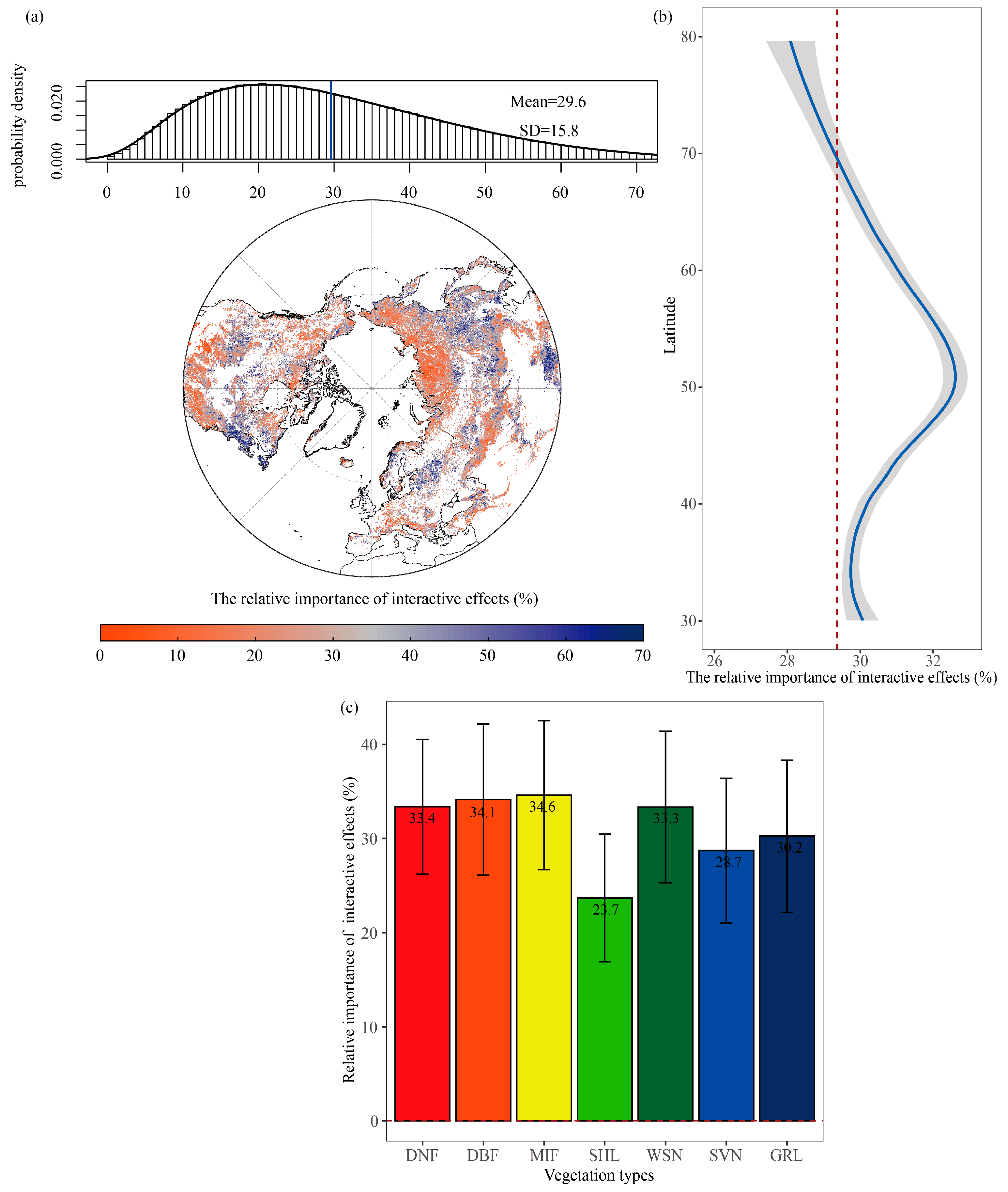
Our results showed that the relative importance of interactive effects (RI_IAE) was 29.6 ± 15.8% over the entire region (Figure 2a). RI_IAE was relatively low in the low latitude of North America and Siberia, while relatively high in Europe, China, and southern Canada. As shown in Figure 2b, RI_IAE increased with the increasing latitude from 30°N–50°N, reaching a maximum at 50°N (approximately 32%), then it gradually decreased when the latitude exceeded 50°N, and was only 28% at 80°N. We also investigated RI_IAE across different biomes (Figure 2c). RI_IAE in the MIF biome was the highest (34.6%), followed by DBF and DNF (34.1% and 33.4%, respectively). RI_IAE in the SHL biome was the lowest (only 23.7%), which was far below the regional average RI_IAE.

3.3. The Key Driving Factors of RVG Trends and Factors Attribution

Figure 3 shows the spatial pattern of the top three drivers of RVG trends and IAE-dominated regions. IAE had dominant contributions to the RVG trends in 11.71% of pixels over the northern extratropics. Our results found that for each pixel over the northern extratropics, CO₂ was the first contributor to RVG trends in 50.98% of pixels, followed by VPD in 18.41% of pixels and GDD in 11.70% of pixels (Figure 3a). That is, the majority of regions, such as North America, Eastern Europe, Central Asia, and China’s Qinghai-Tibet Plateau, can capture a strong influence of rising CO₂ on the RVG trends. As shown in Figure 3b, for the second most significant contribution to the RVG trends in each pixel, the influences of VPD and GDD were comparable (27.24% and 25.19%, respectively), but CO₂ ranked second in only 12.81% of pixels. As shown in Figure 3c, GDD was the third most influential contributor to the RVG trends in 23.86% of pixels, followed by VPD (18.83%) and RD (15.85%). Furthermore, we averaged the first, second, and third contributors to RVG trends over the northern extratropics (Figure 3d), and our findings revealed that CO₂, VPD, and GDD were the primary influences on RVG trends.

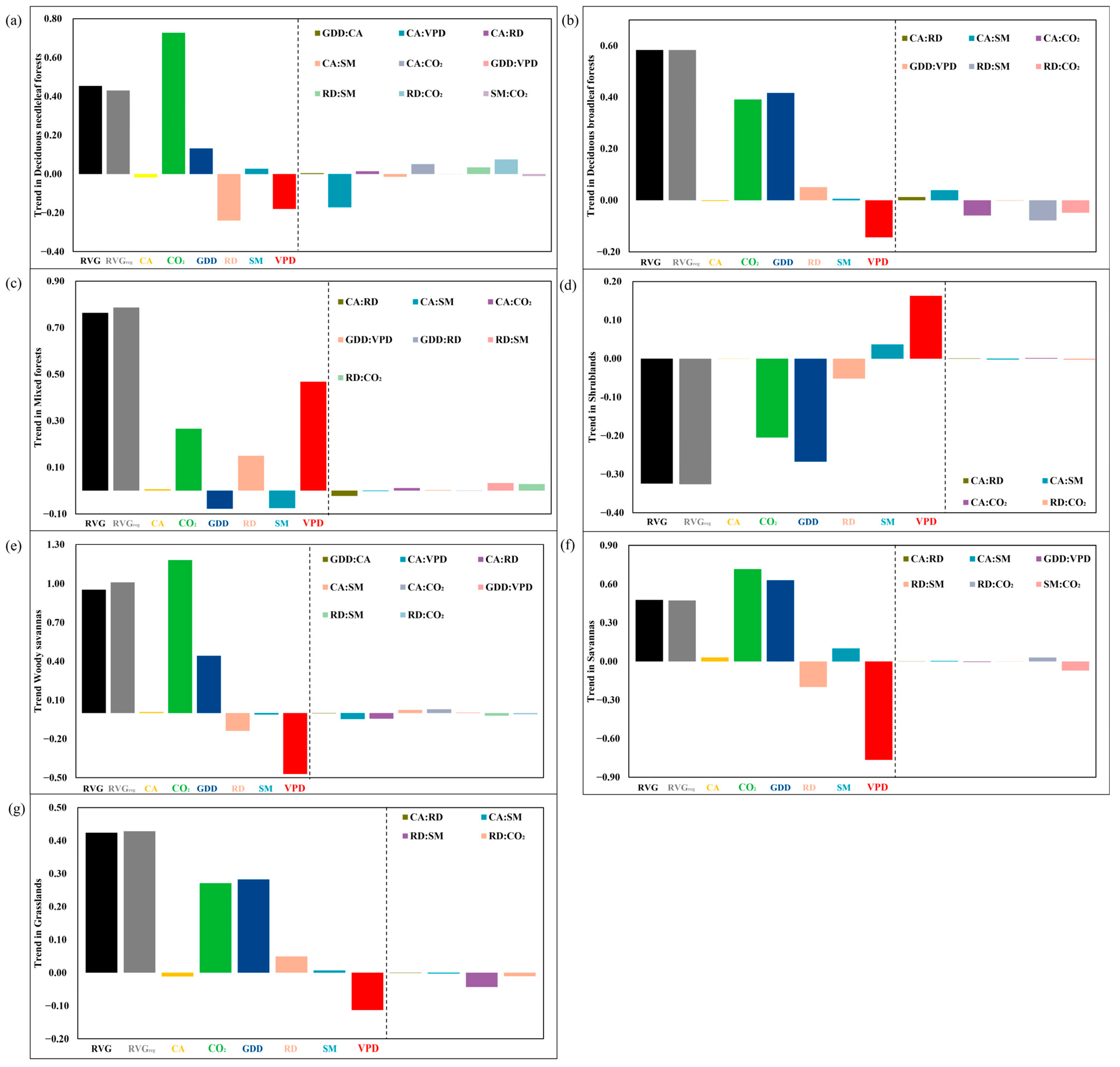
All factors, including environmental variables and interactions between variables, were quantified to help us better understand the driving mechanisms of RVG trends across the different biomes. As shown in Figure 4, the RVG_reg trends could be decomposed into the trends of CA, CO₂, GDD, RD, SM, VPD, and interactive items. The RVG_reg trend in DNF was 0.431% (8-day)⁻¹ decade⁻¹, which was 94.89% of the RVG trend (Figure 4a). The CO₂ trend was the most important driver (0.728% (8-day)⁻¹ decade⁻¹) of the positive RVG_reg trend, slightly strengthened by the GDD trend (0.132% (8-day)⁻¹ decade⁻¹), but partly offset by the RD trend (−0.240% (8-day)⁻¹ decade⁻¹), VPD trend (−0.180% (8-day)⁻¹ decade⁻¹) and the trend of interactions between CA and VPD (−0.172% (8-day)⁻¹ decade⁻¹). The RVG and RVG_reg trends in the DBF biome (Figure 4b) were almost equal (0.583% (8-day)⁻¹ decade⁻¹). The trends of GDD (0.417% (8-day)⁻¹ decade⁻¹) and CO₂ (0.391% (8-day)⁻¹ decade⁻¹) were the primary drivers of the increasing RVG_reg trend, but the VPD trend (−0.144% (8-day)⁻¹ decade⁻¹) and the trends of interactive effects (CA:CO₂, RD:SM, RD:CO₂) partly counteracted the positive RVG_reg trend. The RVG trend and RVG_reg trend in the MIF biome (Figure 4c) were 0.764% and 0.758% (8-day)⁻¹ decade⁻¹, respectively. The VPD trend (0.468% (8-day)⁻¹ decade⁻¹) was the predominant factor of the RVG_reg trend, with the supportive influences of the CO₂ trend and RD trend, at 0.266% and 0.150% (8-day)⁻¹ decade⁻¹, respectively. The RVG and RVG_reg trends (Figure 4d) are negative only in the SHL biome and almost equal at −0.324% (8-day)⁻¹ decade⁻¹. The decelerated RVG_reg was mainly influenced by the GDD trend (−0.267% (8-day)⁻¹ decade⁻¹) and the CO₂ trend (−0.205% (8-day)⁻¹ decade⁻¹), but was partly counteracted by the VPD trend (0.163% (8-day)⁻¹ decade⁻¹). The RVG_reg trend in the WSN biome (Figure 4e) was 0.947% (8-day)⁻¹ decade⁻¹. The CO₂ trend (1.183% (8-day)⁻¹ decade⁻¹) was the most important driver of RVG_reg acceleration, with a supportive influence of the GDD trend (0.443% (8-day)⁻¹ decade⁻¹), but the trends of VPD (−0.472% (8-day)⁻¹ decade⁻¹) and RD (−0.137%% (8-day)⁻¹ decade⁻¹) partly alleviated the positive RVG_reg trend. The RVG and RVG_reg trends in the SVN biome (Figure 4f) were 0.478% and 0.474% (8-day)⁻¹ decade⁻¹, respectively. The trends of CO₂ (0.718% (8-day)⁻¹ decade⁻¹) and GDD (0.631% (8-day)⁻¹ decade⁻¹) were the primary drivers of the increasing RVG_reg trend. However, the VPD trend (−0.765% (8-day)⁻¹ decade⁻¹) strongly counteracted the positive RVG_reg trend. The RVG_reg trend in the GRL biome (Figure 4g) was 0.428% (8-day)⁻¹ decade⁻¹, slightly overestimating the RVG trend (0.424% (8-day)⁻¹ decade⁻¹) by 1%. The GDD trend (0.282% (8-day)⁻¹ decade⁻¹) and CO₂ trend (0.271% (8-day)⁻¹ decade⁻¹) were the key drivers of the positive RVG_reg trend, but the trends of VPD (−0.113% (8-day)⁻¹ decade⁻¹) and the trends of interactions between RD and SM (−0.043% (8-day)⁻¹ decade⁻¹) partly counteracted the positive RVG_reg trend.

4. Discussion

4.1. The Non-Negligible Effects of Interactions between Variables

Previous researchers primarily highlighted the individual effects of variables on the greening rate [2,13,14]. However, vegetation leaf area changes result from the individual effects of variables or the interactions between variables [17]. The influence of environmental variables, such as temperature and CO₂ may be exaggerated, potentially because interactions between variables also significantly affect vegetation growth [40]. Thus, a multivariable regression considering interactions between variables (MRCI), which is suited to analyze the long-term RVG trends, was employed in this study (Figure S1). Our findings showed that the relative importance of interactive effects (RI_IAE) was approximately 30% at both the pixel scale and the biome scale (Figure 3), that is, the relative influence of variable interactions held constant and scarcely varied with scales.

There was a clear latitudinal difference in the relative contribution of interactive effects to the RVG trends. The RI_IAE progressively increased from 30°N to 50°N and peaked at around 50°N, after which it began to fall (Figure 3b). At low or high latitudes, a single climatic variable may be responsible for limiting plant growth or leaf development, rather than interactions between factors. For example, heat or nutrition requirements can directly determine plant growth and dispersal in high-latitude tundra ecosystems [41].

Despite the relatively strong interaction effects, our analysis indicated that IAE (Figure 3) only had dominant contributions (RI_IAE > 50%) to the vegetation greening rate trends in 11.71% of pixels over the northern extratropics. The contribution values of different variable interactions to RVG trends at the biome scale can be positive or negative (Figure 4), so the cumulative results may offset the part of the influence of interactions. For example, the interactions between temperature and water availability have different effects for plants. If warming enhances the drought risk of the ecosystem, the increasing evaporation will enhance soil water consumption and exacerbate drought conditions for plants [21]. When light conditions are sufficient and not a limiting factor, temperature and VPD will jointly affect the rate of photosynthesis, that is, suitable warming and slightly increased VPD are beneficial for plant growth [42]. Nonetheless, the negative effect of interactions between CA and VPD in the deciduous broadleaf forest was comparable with that of VPD, and the interaction between RD and SM in grasslands was approximately half of the role of VPD. The contributions of interactive items were negative in most biomes, indicating that variable interactions can regulate vegetation greening rate acceleration in those biomes.

4.2. Elevated CO₂, Enhanced VPD, and Warming Strongly Affect the RVG Trends

Whether at the pixel scale or across distinct biomes, rising CO₂, enhanced VPD, and warming were the common and primary drivers affecting the RVG trends. Our analyses showed that rising CO₂ was the first contributor to RVG trends in 50.98% pixels over the northern extratropics. The rising CO₂ strongly influenced RVG trends in all vegetation types, especially deciduous needleleaf forests and woody savannas. Generally, rising CO₂ concentrations can increase branching and promote leaf development [36].

Previous studies reported that the rising CO₂ explained 70% of the LAI greening trend at the global scale [17], and was the highest contributer (59.5% ± 26.6%) to the increasing trends of vegetation productivity [22]. Because RVG was derived from LAI, the strong CO₂ effect from the findings of this study appears to be consistent with these reports. However, the effects of CO₂ fertilization on vegetation greening rate differ from that of LAI and vegetation productivity, and the current literature on free-air CO₂ enrichment (FACE) has not identified plausible links between CO₂ and the spring greening rate. As a result, the effects of CO₂ on RVG should be explored further using FACE experiments or multi-source remote sensing and site observation data.

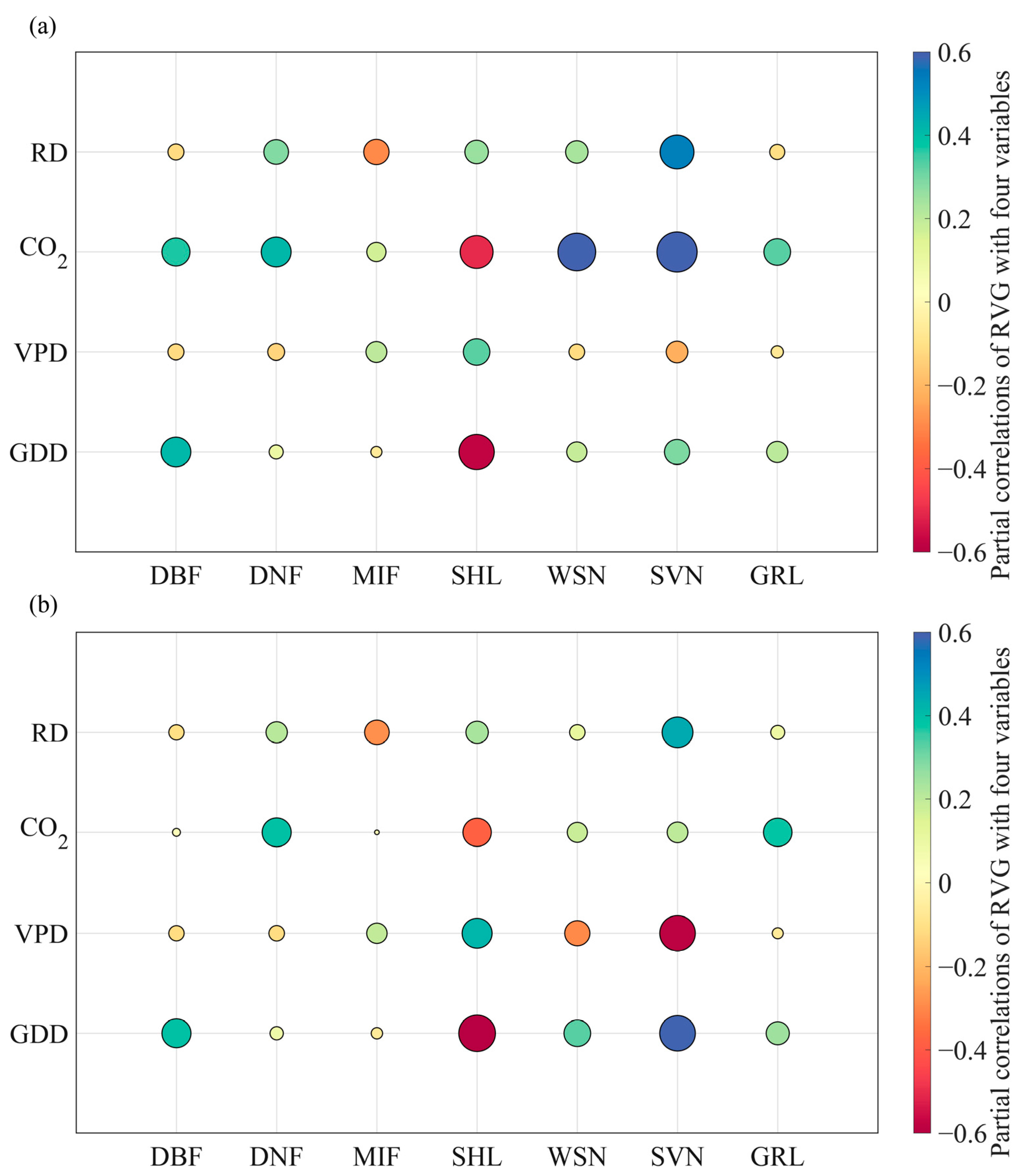
Remarkably, although CO₂ was found to play a key role in the long-term RVG trends, we must be cautious in identifying this influence because CO₂ concentration has been continuously increasing for several decades. It can be a result of misinterpretation due to the common linear trends in the RVG and CO₂ concentration. Here, we added partial correlations between the RVG and four independent variables (Figure 5) to show the interannual relationships of those variables. After removing the linear trend, the partial correlation coefficient between CO₂ and RVG reduced significantly, especially in DBF, WSN and SVN biomes. That is, the influence of CO₂ on RVG trends was overestimated in this study; however, CO₂ remains particularly important in GRL and DNF biomes.

According to our findings, the relative importance of atmospheric drought (VPD) ranked in the top three driving factors in each pixel, affecting 18.41%, 27.24%, and 18.83% of pixels, respectively (Figure 3). The RVG trends were strongly influenced by increased VPD in arid and semi-arid climatic zones, especially in the water-limited ecosystems, such as woody savannas, savannas, and grasslands (Figure 4). That is, the enhanced VPD could play a crucial role in alleviating RVG acceleration that is caused by warming and rising atmospheric CO₂ concentrations. Thus, the RVG trends would not constantly rise with warming and rising CO₂ concentrations because enhanced VPD could cause higher evaporative demand of plants, and extremely high VPD would trigger stomatal closure, resulting in an inefficient photosynthesis rate and restrained leaf development [21,43], especially in a water-limited ecosystem.

As one of the top three variables in each pixel, the GDD trend (warming) affected 11.79%, 25.19%, and 23.80% of pixels over the northern extratropics, respectively. Warming was also the main driver in most biomes, especially in deciduous broadleaf forests, shrublands, and grasslands (Figure 4), which is consistent with the high correlation between accelerating RVG and warming reported in previous studies [2,44]. Temperature-dependent enzymatic catalytic reactions can accelerate plant growth and foliage development under warming [20,45], thus foliar development is highly affected by rising temperature in the form of rapid leaf expansion [46].

In the deciduous needleleaf forests, the decreased solar radiation and enhanced VPD partly offset the influences of the sharp rise of CO₂ concentrations, suggesting that the accelerating greening rate in high-latitude ecosystems is restrained by the trends of radiation and moisture. Zhang et al. [47] indicated that radiation restriction will become increasingly important both in spring and autumn for vegetation growth, particularly in high latitude regions. The enhanced VPD partly offset the influence of rising CO₂ concentrations and warming on the RVG deceleration in shrublands, which contradicts prior findings that RVG acceleration was linked to warming and elevated CO₂. We found that the RVG in shrublands was negatively correlated with temperature and CO₂, and positively correlated with VPD (Figure 5). This may be related to the fact that we merged open shrublands and closed shrublands into shrublands, and thus the partial correlation analysis wrongly described the relationship between RVG and climate variables. The driving mechanism in the mixed forests was a mystery, since this result indicated that enhanced VPD contributed to the RVG acceleration. However, plants are usually constrained by water availability, and VPD has a detrimental influence on leaf development [48]. The positive effect of VPD in this study may be attributed to the incorrect relationship between the greening rate and VPD caused by the mixed vegetation types.

4.3. Limitations and Future Work

We investigated the effects of environmental variables and variable interactions on RVG trends, however only the product of two variables was included in the interactions. Given the intricacy of the interactions, our model may not fully reveal the complex interactions among multiple environmental factors, and may have underestimated the influence of interactions to the vegetation greening rate trends. In addition, previous studies suggested that the limitation of nitrogen and phosphorus availability shifted northern vegetation changes [26,49]. Human land management also plays a considerable role in the vegetation greening rate [22]. Therefore, future works should comprehensively consider anthropogenic influence and nutrient availability, and effectively distinguish the individual and interactive effects of various factors on vegetation phenology.

5. Conclusions

We investigated the rate of vegetation green-up trends over the northern extratropics in this study. We discovered a non-negligible influence of interactions between variables on the RVG trends (approximately 30%) at both the pixel scale and the biome scale using a multivariable regression considering interactions between variables. Our findings suggest that in addition to warming, elevated CO₂ and enhanced VPD also significantly affect RVG trends. Additionally, the increasing atmospheric aridity in the majority of biomes could alleviate the RVG acceleration. Quantifying the effects of variable interactions and clarifying the underlying mechanisms causing the changes in RVG trends across different biomes will help us to better understand vegetation spring green-up under global changes.

References

1. Bonan, G.B. Forests and climate change: Forcings, feedbacks, and the climate benefits of forests. Science 2008, 320, 1444–1449. [Google Scholar] [CrossRef]
2. Park, H.; Jeong, S.; Penuelas, J. Accelerated rate of vegetation green-up related to warming at northern high latitudes. Glob. Change Biol. 2020, 26, 6190–6202. [Google Scholar] [CrossRef]
3. Piao, S.L.; Wang, X.H.; Park, T.; Chen, C.; Lian, X.; He, Y.; Bjerke, J.W.; Chen, A.P.; Ciais, P.; Tommervik, H.; et al. Characteristics, drivers and feedbacks of global greening. Nat. Rev. Earth Environ. 2020, 1, 14–27. [Google Scholar] [CrossRef]
4. Badeck, F.W.; Bondeau, A.; Bottcher, K.; Doktor, D.; Lucht, W.; Schaber, J.; Sitch, S. Responses of spring phenology to climate change. New Phytol. 2004, 162, 295–309. [Google Scholar] [CrossRef]
5. Buitenwerf, R.; Rose, L.; Higgins, S.I. Three decades of multi-dimensional change in global leaf phenology. Nat. Clim. Change 2015, 5, 364–368. [Google Scholar] [CrossRef]
6. Schwartz, M.D.; Ahas, R.; Aasa, A. Onset of spring starting earlier across the Northern Hemisphere. Glob. Change Biol. 2006, 12, 343–351. [Google Scholar] [CrossRef]
7. Garonna, I.; De Jong, R.; De Wit, A.J.W.; Mucher, C.A.; Schmid, B.; Schaepman, M.E. Strong contribution of autumn phenology to changes in satellite-derived growing season length estimates across Europe (1982–2011). Glob. Change Biol. 2014, 20, 3457–3470. [Google Scholar] [CrossRef]
8. Gonsamo, A.; Chen, J.M.; Ooi, Y.W. Peak season plant activity shift towards spring is reflected by increasing carbon uptake by extratropical ecosystems. Glob. Change Biol. 2018, 24, 2117–2128. [Google Scholar] [CrossRef]
9. Gu, L.; Post, W.M.; Baldocchi, D.; Black, T.A.; Verma, S.B.; Vesala, T.; Wofsy, S.C. Phenology of vegetation photosynthesis. Phenol. Integr. Environ. Sci. 2003, 39, 467–485. [Google Scholar]
10. Seyednasrollah, B.; Swenson, J.J.; Domec, J.-C.; Clark, J.S. Leaf phenology paradox: Why warming matters most where it is already warm. Remote Sens. Environ. 2018, 209, 446–455. [Google Scholar] [CrossRef]
11. Jeong, S.J.; Medvigy, D.; Shevliakova, E.; Malyshev, S. Uncertainties in terrestrial carbon budgets related to spring phenology. J. Geophys. Res. Biogeosci. 2012, 117, G01030. [Google Scholar] [CrossRef]
12. Keenan, T.F.; Gray, J.; Friedl, M.A.; Toomey, M.; Bohrer, G.; Hollinger, D.Y.; Munger, J.W.; O’Keefe, J.; Schmid, H.P.; SueWing, I.; et al. Net carbon uptake has increased through warming-induced changes in temperate forest phenology. Nat. Clim. Change 2014, 4, 598–604. [Google Scholar] [CrossRef]
13. Kern, A.; Marjanovic, H.; Barcza, Z. Spring vegetation green-up dynamics in Central Europe based on 20-year long MODIS NDVI data. Agric. For. Meteorol. 2020, 287, 107969. [Google Scholar] [CrossRef]
14. Park, H.; Jeong, S.J.; Ho, C.H.; Kim, J.; Brown, M.E.; Schaepman, M.E. Nonlinear response of vegetation green-up to local temperature variations in temperate and boreal forests in the Northern Hemisphere. Remote Sens. Environ. 2015, 165, 100–108. [Google Scholar] [CrossRef]
15. Wang, S.H.; Zhang, Y.G.; Ju, W.M.; Chen, J.M.; Ciais, P.; Cescatti, A.; Sardans, J.; Janssens, I.A.; Wu, M.S.; Berry, J.A.; et al. Recent global decline of CO2 fertilization effects on vegetation photosynthesis. Science 2020, 370, 1295–1300. [Google Scholar] [CrossRef]
16. Kohlmaier, G.H.; Siré, E.-O.; Janecek, A.; Keeling, C.D.; Piper, S.C.; Revelle, R. Modelling the seasonal contribution of a CO2 fertilization effect of the terrestrial vegetation to the amplitude increase in atmospheric CO2 at Mauna Loa Observatory. Tellus B Chem. Phys. Meteorol. 2017, 41, 487–510. [Google Scholar] [CrossRef]
17. Zhu, Z.; Piao, S.; Myneni, R.B.; Huang, M.; Zeng, Z.; Canadell, J.G.; Ciais, P.; Sitch, S.; Friedlingstein, P.; Arneth, A.; et al. Greening of the Earth and its drivers. Nat. Clim. Change 2016, 6, 791–795. [Google Scholar] [CrossRef]
18. Fu, Y.S.H.; Zhao, H.F.; Piao, S.L.; Peaucelle, M.; Peng, S.S.; Zhou, G.Y.; Ciais, P.; Huang, M.T.; Menzel, A.; Uelas, J.P.; et al. Declining global warming effects on the phenology of spring leaf unfolding. Nature 2015, 526, 104. [Google Scholar] [CrossRef]
19. Rollinson, C.R.; Kaye, M.W. Experimental warming alters spring phenology of certain plant functional groups in an early successional forest community. Glob. Change Biol. 2012, 18, 1108–1116. [Google Scholar] [CrossRef]
20. Wolkovich, E.M.; Cook, B.I.; Allen, J.M.; Crimmins, T.M.; Betancourt, J.L.; Travers, S.E.; Pau, S.; Regetz, J.; Davies, T.J.; Kraft, N.J.B.; et al. Warming experiments underpredict plant phenological responses to climate change. Nature 2012, 485, 494–497. [Google Scholar] [CrossRef]
21. Yuan, W.P.; Zheng, Y.; Piao, S.L.; Ciais, P.; Lombardozzi, D.; Wang, Y.P.; Ryu, Y.; Chen, G.X.; Dong, W.J.; Hu, Z.M.; et al. Increased atmospheric vapor pressure deficit reduces global vegetation growth. Sci. Adv. 2019, 5, eaax1396. [Google Scholar] [CrossRef] [PubMed]
22. Wang, L.H.; Tian, F.; Wang, Y.H.; Wu, Z.D.; Schurgers, G.; Fensholt, R. Acceleration of global vegetation greenup from combined effects of climate change and human land management. Glob. Change Biol. 2018, 24, 5484–5499. [Google Scholar] [CrossRef] [PubMed]
23. Clark, J.S.; Salk, C.; Melillo, J.; Mohan, J. Tree phenology responses to winter chilling, spring warming, at north and south range limits. Funct. Ecol. 2014, 28, 1344–1355. [Google Scholar] [CrossRef]
24. Cook, B.I.; Wolkovich, E.M.; Parmesan, C. Divergent responses to spring and winter warming drive community level flowering trends. Proc. Natl. Acad. Sci. USA 2012, 109, 9000–9005. [Google Scholar] [CrossRef] [PubMed]
25. Peñuelas, J.; Ciais, P.; Canadell, J.G.; Janssens, I.; Fernández-Martínez, M.; Carnicer, J.; Obersteiner, M.; Piao, S.; Vautard, R.; Sardans, J. Shifting from a fertilization-dominated to a warming-dominated period. Nat. Ecol. Evol. 2017, 1, 1438–1445. [Google Scholar] [CrossRef] [PubMed]
26. Terrer, C.; Jackson, R.B.; Prentice, I.C.; Keenan, T.F.; Kaiser, C.; Vicca, S.; Fisher, J.B.; Reich, P.B.; Stocker, B.D.; Hungate, B.A.; et al. Nitrogen and phosphorus constrain the CO2 fertilization of global plant biomass. Nat. Clim. Change 2019, 9, 684–689. [Google Scholar] [CrossRef]
27. Reich, P.; Hobbie, S.; Lee, T. Plant growth enhancement by elevated CO2 eliminated by joint water and nitrogen limitation. Nat. Geosci. 2014, 7, 920–924. [Google Scholar] [CrossRef]
28. Wang, L.; Fensholt, R. Temporal Changes in Coupled Vegetation Phenology and Productivity are Biome-Specific in the Northern Hemisphere. Remote Sens. 2017, 9, 1277. [Google Scholar] [CrossRef]
29. Xiao, Z.; Liang, S.; Wang, J.; Chen, P.; Yin, X.; Zhang, L.; Song, J. Use of General Regression Neural Networks for Generating the GLASS Leaf Area Index Product from Time-Series MODIS Surface Reflectance. IEEE Trans. Geosci. Remote Sens. 2014, 52, 209–223. [Google Scholar] [CrossRef]
30. Xiao, Z.; Liang, S.; Jiang, B. Evaluation of four long time-series global leaf area index products. Agric. For. Meteorol. 2017, 246, 218–230. [Google Scholar] [CrossRef]
31. Xu, B.; Li, J.; Park, T.; Liu, Q.; Zeng, Y.; Yin, G.; Zhao, J.; Fan, W.; Yang, L.; Knyazikhin, Y.; et al. An integrated method for validating long-term leaf area index products using global networks of site-based measurements. Remote Sens. Environ. 2018, 209, 134–151. [Google Scholar] [CrossRef]
32. Hansen, M.C.; Defries, R.S.; Townshend, J.R.G.; Sohlberg, R. Global land cover classification at 1km spatial resolution using a classification tree approach. Int. J. Remote Sens. 2000, 21, 1331–1364. [Google Scholar] [CrossRef]
33. Hersbach, H.; Bell, B.; Berrisford, P.; Hirahara, S.; Horanyi, A.; Munoz-Sabater, J.; Nicolas, J.; Peubey, C.; Radu, R.; Schepers, D.; et al. The ERA5 global reanalysis. Q. J. R. Meteorol. Soc. 2020, 146, 1999–2049. [Google Scholar] [CrossRef]
34. Rödenbeck, C. Estimating CO2 Sources and Sinks from Atmospheric Mixing Ratio Measurements Using a Global Inversion of Atmospheric Transport; Technical Report 6; Max Planck Institute for Biogeochemistry: Jena, Germany, 2005. [Google Scholar]
35. Caffarra, A.; Donnelly, A. The ecological significance of phenology in four different tree species: Effects of light and temperature on bud burst. Int. J. Biometeorol. 2011, 55, 711–721. [Google Scholar] [CrossRef] [PubMed]
36. Prtchard, S.G.; Rogers, H.H.; Prior, S.A.; Peterson, C.M. Elevated CO2 and plant structure: A review. Glob. Change Biol. 1999, 5, 837–907. [Google Scholar] [CrossRef]
37. Zeng, L.; Wardlow, B.D.; Xiang, D.; Hu, S.; Li, D. A review of vegetation phenological metrics extraction using time-series, multispectral satellite data. Remote Sens. Environ. 2020, 237, 111511. [Google Scholar] [CrossRef]
38. Gonsamo, A.; Chen, J.M.; D’Odorico, P. Deriving land surface phenology indicators from CO2 eddy covariance measurements. Ecol. Indic. 2013, 29, 203–207. [Google Scholar] [CrossRef]
39. Balli, H.O.; Sorensen, B.E. Interaction effects in econometrics. Empir. Econ. 2013, 45, 583–603. [Google Scholar] [CrossRef]
40. Liu, H.Y.; Jiao, F.S.; Yin, J.Q.; Li, T.Y.; Gong, H.B.; Wang, Z.Y.; Lin, Z.S. Nonlinear relationship of vegetation greening with nature and human factors and its forecast—A case study of Southwest China. Ecol. Indic. 2019, 111, 106009. [Google Scholar] [CrossRef]
41. Williams, J.R.; Zelalem, A.M.; Tang, J.Y.; Zhu, Q.; Nicholas, J.B.; Robert, F.G. Non-growing season plant nutrient uptake controls Arctic tundra vegetation composition under future climate. Environ. Res. Lett. 2019, 61, 7. [Google Scholar]
42. Sullivan, N.H.; Bolstad, P.V.; Vose, J.M. Estimates of net photosynthetic parameters for twelve tree species in mature forests of the southern Appalachians. Tree Physiol. 1996, 16, 397. [Google Scholar] [CrossRef] [PubMed]
43. Novick, K.A.; Ficklin, D.L.; Stoy, P.C.; Williams, C.A.; Bohrer, G.; Oishi, A.C.; Papuga, S.A.; Blanken, P.D.; Noormets, A.; Sulman, B.N.; et al. The increasing importance of atmospheric demand for ecosystem water and carbon fluxes. Nat. Clim. Change 2016, 6, 1023–1027. [Google Scholar] [CrossRef]
44. Qiu, T.; Song, C.; Clark, J.S.; Seyednasrollah, B.; Rathnayaka, N.; Li, J.X. Understanding the continuous phenological development at daily time step with a Bayesian hierarchical space-time model: Impacts of climate change and extreme weather events. Remote Sens. Environ. 2020, 247, 111956. [Google Scholar] [CrossRef]
45. Atkinson, D.; Porter, J.R. Temperature, plant development and crop yields. Trends Plant Sci. 1996, 1, 119–124. [Google Scholar] [CrossRef]
46. Way, D.A.; Oren, R. Differential responses to changes in growth temperature between trees from different functional groups and biome: A review and synthesis of data. Tree Physiol. 2010, 30, 669–688. [Google Scholar] [CrossRef] [PubMed]
47. Zhang, Y.; Commane, R.; Zhou, S.; Williams, A.P.; Gentine, P. Light limitation regulates the response of autumn terrestrial carbon uptake to warming. Nat. Cliam. Change 2020, 10, 739–743. [Google Scholar] [CrossRef]
48. Grossiord, C.; Buckley, T.N.; Cernusak, L.A.; Novick, K.A.; Poulter, B.; Siegwolf, R.T.W.; Sperry, J.S.; McDowell, N.G. Plant responses to rising vapor pressure deficit. New Phytol. 2020, 226, 1550–1566. [Google Scholar] [CrossRef]
49. Elmore, A.J.; Nelson, D.M.; Craine, J.M. Earlier springs are causing reduced nitrogen availability in North American eastern deciduous forests. Nat. Plants 2016, 2, 16133. [Google Scholar] [CrossRef]
Figure 1. Spatial distribution of (a) seven vegetation types including deciduous needleleaf forests (DNF), deciduous broadleaf forests (DBF), mixed forests (MIF), shrublands (SHL), woody savannas (WSN), savannas (SVN), and grasslands (GRL); (b) RVG trends over northern extratropics (the area-weighted average RVG and its trend are marked in the upper left corner, and the proportion of positive and negative trends is shown in the lower left corner. N and P represent a negative trend and a positive trend, respectively); (c) RVG trends across different biomes during the period 1981–2018.
Remotesensing 14 03946 g001
Figure 2. (a) The spatial distribution of the relative importance of interactive effects (RIIAE) on the RVGreg trends over the northern extratropics. RIIAE (b) along the latitudinal gradient and (c) across different biomes including deciduous needleleaf forests (DNF), deciduous broadleaf forests (DBF), mixed forests (MIF), shrublands (SHL), woody savannas (WSN), savannas (SVN), and grasslands (GRL).
Remotesensing 14 03946 g002
Figure 3. Spatial distribution of the drivers of RVG trends, defined as the driving factor that contributes (a) first, (b) second, and (c) third to the RVG trends in each pixel over the northern extratropics. (d) The fraction of pixel (%) for the key factors (note: IAE indicates that the relative importance of the interactive effects (RIIAE) exceeds 50% (meaning the interactions are dominant), so its percentage remains constant).
Remotesensing 14 03946 g003
Figure 4. The bars in the graphs represent RVG trends, RVGreg trends and the contribution of CA, CO2, GDD, RD, SM, VPD, and interactive items (right of the dotted line) in the (a) DNF, (b) DBF, (c) MIF, (d) SHL, (e) WSN, (f) SVN, and (g) GRL biomes.
Remotesensing 14 03946 g004
Figure 5. Partial correlation of RVG with RD, CO2, VPD, and GDD (a) before detrending variables, and (b) after detrending variables across different biomes including deciduous needleleaf forests (DNF), deciduous broadleaf forests (DBF), mixed forests (MIF), shrublands (SHL), woody savannas (WSN), savannas (SVN), and grasslands (GRL) for the period from 1981 to 2018.
Remotesensing 14 03946 g005
Publisher’s Note: MDPI stays neutral with regard to jurisdictional claims in published maps and institutional affiliations.