Sensitivity Analysis of Ozone Profiles Retrieved from SCIAMACHY Limb Radiance Based on the Weighted Multiplicative Algebraic Reconstruction Technique

Abstract

A detailed sensitivity analysis of ozone density profile retrieval was applied to scattering solar radiance spectra measured with the SCanning Imaging Absorption spectroMeter for Atmospheric CHartographY (SCIAMACHY) instrument aboard the ENVIronmental SATellite (ENVISAT). The vertical density distribution of ozone between 10 and 69 km was obtained using the weighted multiplicative algebraic reconstruction technique and the radiative transfer model for SCIAMACHY. This study investigates the error sources for the retrieved ozone profiles, which are relevant to explain the difference between two independent instruments. The numerical simulation method was adapted to quantify the impact of various error sources on the retrieval accuracy of ozone profiles. First, the tangent height (TH) registration was found to be the largest error source. Assuming an aerosol-free atmosphere, under the condition of background aerosol, the ozone profile showed a negative deviation of ~2–10% below 40 km. With an incorrect a priori profile, ozone estimates may result in a 5–10% average error at the upper and lower boundaries. The ozone retrieval error caused by the uncertainty of surface albedo, ozone absorption cross-section, temperature, pressure profile, and low clouds was relatively small. The random error caused by the disturbance of the measurement vector obeying a Gaussian distribution did not exceed 5%. Second, the estimation of various error sources for different solar zenith angles was investigated. The error sources most strongly dependent on SZAs were aerosols, surface albedo, and clouds. Finally, the error estimation of the ozone retrieval between the northern hemisphere (NH) and the southern hemisphere (SH) was investigated, revealing that there were no strong interhemispheric differences, except for cloud height. These results can be used for interpretation of instrumental comparisons and validation of SCIAMACHY ozone profiles retrieved from different algorithms in a rigorous manner.

1. Introduction

Ozone, an important atmospheric trace gas, can absorb strong ultraviolet (UV) radiation, acting as a protective layer for the earth’s surface and playing a vital role in regulating stratosphere radiation and affecting both atmospheric circulation and climate [1]. Ozone-related research has expanded since the discovery of the Antarctic spring ozone hole and the depletion of stratospheric ozone by the anthropogenic release of chlorofluorocarbons (CFCs) [2,3].

Although the chemical properties of stratospheric ozone are well understood, a better assessment of the expected ozone recovery [4], stratospheric circulation, temperature responses to the increase in greenhouse gases [5], and the long-term ozone trend require reliable long-term data sets from both ground and satellite instruments [1].

Over the past few decades, remote sensing techniques have been used to determine ozone concentrations at various atmospheric layers [6]. For example, traditional space borne instruments in nadir viewing, such as the Global Ozone Monitoring Experiment II (GOME-2) [7], the Solar Backscatter Ultraviolet Sounder (SBUS) [8], the Ozone Monitoring Instrument (OMI) [9], and the Environmental trace gases Monitoring Instrument (EMI) [10], have shown a better global distribution of the total column of ozone and other trace gases. Satellites observing in solar occultation mode, such as the Global Ozone Monitoring by Occultation of Stars (GOMOS) instrument [11] and the Atmospheric Chemistry Experiment-Fourier Transform Spectrometer (ACE-FTS) [12], can derive an ozone profile with a high vertical resolution. However, occultation measurements suffer from poor geographical coverage because of the limited occultation condition. Satellite observations of scattered solar radiation in the limb observation geometry are one of the standard techniques for measuring stratospheric ozone profiles and other minor atmospheric components. Limb-scattering data sets allow the retrieval of trace gas profiles at a vertical resolution comparable to occultation measurements but have significantly better global coverage [13]. Limb-scattering technology was successfully used for the first time by the Shuttle Ozone Limb Sounding Experiment/Limb Ozone Retrieval Experiment (SOLSE/LORE) instrument onboard the STS-87 space shuttle mission, launched by NASA in 1997 [14]. Subsequently, instruments with limb ultraviolet (UV), visible, near infrared (NIR), and short wave infrared (SWIR) scattering sounding technology were employed, including the Optical Spectrograph and InfraRed Imaging System (OSIRIS) launched onboard the Odin satellite in February 2001 [15], the SCanning Imaging Absorption spectroMeter for Atmospheric CHartographY (SCIAMACHY) launched in March 2002 onboard the Environmental Satellite (ENVISAT) [16], the Stratospheric Aerosols and Gas Experiment (SAGE) III instrument launched onboard the Meteor-3M aircraft in 2004 [17], and the Ozone Mapping and Profiler Suite (OMPS) instruments launched onboard the Suomi National Polar-orbiting Partnership (SNPP) platform in October 2011 [18].

The primary source of limb-scattering radiance is the single or multiple scattering sunlight of the atmospheric and surface reflection, which is affected by clouds, aerosols, and surface albedo. Calculating the concentration of ozone using limb-scattering radiance is a retrieval process that requires complex radiative transfer model computation, and the uncertainty on several atmospheric parameters contributes to the errors on the retrieved profiles. Von Savigny et al., summarized the results of an error analysis for an ozone retrieval algorithm based on the optimal estimation of nonlinear Newton iterations, including the error budget of surface albedo, stratospheric aerosols, background atmospheric interference, cloud effects, and instrument noise [19]. However, the algorithm did not estimate errors that result from tangent height (TH) misregistration, despite Loughman et al., indicating the TH misregistration as the largest source of ozone retrieval error [20]. Roth et al., proposed a method for retrieving ozone profiles using two Chappuis triplet vectors (CTVs) from measurements of the Odin/OSIRIS instrument. This method is applicable on the basis of analyzing the dependence of iterations, an initial guess profile, the number of orders of multiple scatter, and instrument noise effect on ozone retrieval [21]. Sonkaew et al., studied the influence of cloud parameter uncertainty on the retrieved SCIAMACHY ozone profile, revealing that the most influential parameters on ozone retrieval were cloud optical thickness, ground albedo, and solar zenith angle [22]. For OSIRIS, von Savigny et al., introduced sensitivity studies of stratospheric ozone retrievals including spectrometer polarization, as well as internal and external stray light—besides common error sources—revealing an estimated total error of ~10% between 15 and 40 km [23]. Wang subsequently studied the effects of surface albedo, aerosols, TH, and clouds on the retrieval of ozone profiles from the SCIAMACHY limb observations [24]. However, the impact of the a priori knowledge on the retrievals was not investigated. Rahpoe et al., studied the influence of additional physical parameters on ozone profile retrievals using the radiative transfer model (RTM) for SCIAMACHY (SCIATRAN), where potential uncertainties were derived from errors of different parameters in the forward model, whereas the total random error (10–15% for most stratospheric ozone profiles) and systematic error (7%) of the SCIAMACHY limb ozone profile were defined [25]. Rault et al., described a retrieval algorithm in which estimates of bias and random errors were presented [18]. Biases are primarily derived from spectral uncertainty and model error, whereas random errors were mostly attributed to measurement noise, TH registration uncertainty, intermediate product retrieval errors (i.e., aerosol extinction, NO₂, cloud effects, and surface reflectance), and instrumental effects (stray light, 2-D gridding, and consolidation). Arosio et al. [1] later retrieved ozone profiles from limb observations performed by the OMPS instrument. The square roots of the diagonal elements for the retrieval noise covariance matrix were referred to as the theoretical precision of the retrieval. However, smoothing errors were not included in the retrieval error budget. Ultimately, the retrieval error caused by measurement noise was 1–4% above 25 km and 10–30% in the upper troposphere. Zhu et al., studied a method based on wavelength pairing and the multiplicative algebraic reconstruction technique (MART) for retrieving ozone profiles from SCIAMACHY limb radiance and analyzed the effects of an a priori profile, multiple iterations, TH, and NO₂ concentrations on retrieval values [26]. Von Clarmann et al., proposed a common framework for the appropriate communication of uncertainty and other measurement characteristics, and provided a list of recommendations that should help to unify retrieval error reporting [27].

Thus, a detailed error characterization is useful for a meaningfully interpreting the verification results obtained by comparing the collocated ozone vertical distribution datasets between independent instruments. Therefore, the current study provides a theoretical basis for the ozone-retrieved algorithm based on the weighted multiplicative algebraic reconstruction technique (WMART) and describes the algorithm’s sensitivity to various disturbances. Furthermore, changes in various error sources within the ozone profile retrievals from the SCIAMACHY limb radiance at different solar zenith angles (SZAs) were studied, and the differences between the northern and southern hemispheres are presented.

This paper is structured as follows: Section 2 describes the retrieval scheme based on wavelength pairing and the WMART algorithm, in addition to introducing the software package SCIATRAN; Section 3 introduces the error analysis method for ozone retrieval based on the numerical perturbation method; Section 4 and Section 5 provide a summary and discussion of the results, respectively; the conclusions are provided in Section 6.

2. Materials and Retrieval Method

2.1. Instrumentation Overview and Datasets Used for Experiments

SCIAMACHY is one of the ten scientific instruments carried onboard ENVISAT. This satellite was launched into a sun synchronous orbit at about 800 km altitude on 1 March 2002 (concluded May 2012), with an inclination of 98.55°, and an ascending node at GMT 10:00. The SCIAMACHY instrument observed the transmitted, reflected, and scattered solar radiation in the UV-VIS-NIR bands, while detecting the concentration and distribution of atmospheric parameters, such as trace gases, aerosols, temperature, and clouds. The instrument measured in eight spectral channels over the 214–2386 nm range, with a spectral resolution of 0.24–1.48 nm. In the limb observation geometry, the SCIAMACHY instrument observed the atmosphere 3280 km ahead of the flight direction. The line-of-sight of the instrument passed through the atmosphere along a slanted line, and the scattered photons from the sunlight were detected and transmitted to the instrument’s field of view. A typical SCIAMACHY limb scanning sequence started from the surface and stepped upward with a vertical resolution of ~3.3 km to a maximum height of ~90 km. The horizontal scanning time of each tangent point was ~1.5 s. The satellite advanced 400 km in the orbital direction within one limb scanning period, and the orbital operation cycle was 100.6 min, thereby achieving global coverage within six days. Detailed information on the SCIAMACHY instruments has been reported by Bovensmann et al. [16].

According to Wang et al. [28], limb radiance rarely changes with solar azimuth angles, but it significantly changes with SZAs. Figure 1a shows the variation in SZA with latitude in different seasons, whereas Figure 1b shows the SZAs of the different orbits on the same day. Evidently, the SZAs of the SCIAMACHY limb observation geometry increased with increasing latitude in the northern and southern hemispheres, depicting its seasonal dependence. Therefore, the sensitivity analysis of the ozone profile retrieval considered different SZAs. In Section 4, the contributions of each error term with SZAs have been introduced in an example case using the mid-latitudes of the northern hemisphere (NH) (average 35°N, 140°E), and the viewing geometry was taken from SCIAMACHY orbit 49255.

Figure 2 shows an example of the SCIAMACHY limb profiles at different latitudes and their corresponding SZAs. The limb radiance profiles under different SZAs show marked differences, but all had a similar profile shape in UV or VIS bands. However, in the same SZA, compared with Figure 2a, differences in the profiles between the northern and the southern hemispheres were relatively small (Figure 2b). In addition to analyzing the variation in the error term with SZAs, an error analysis of the northern and southern hemispheres was conducted under the same latitude band. The sensitivity was calculated for 10 days in 2011, including 165 NH profiles and 157 SH profiles, with latitudes ranging from 30° to 40°. In Section 4.3, the errors of the northern and southern hemispheres are presented as the average of the errors calculated from different profiles in 2011.

2.2. Description of Retrieval Method

Here, the vertical distribution of ozone between 10 and 69 km was retrieved from limb data in the UV and visible absorption bands of ozone. As the first step in retrieving the ozone profile from the limb measurements, the sensitivity of the limb-scattering radiance at different wavelengths must be correlated with the change in ozone density. The radiance of the UV limb provides ozone profile information at altitudes >35 km, whereas visible limb data are required to retrieve ozone profiles <35 km. To reduce the sensitivity to interference species without sacrificing ozone sensitivity [20], two main methods to process the measured limb data were used here, namely radiance normalization and wavelength pairing.

2.2.1. Radiance Normalization

To reduce instrument calibration error and the influence of light scattering in the lower atmosphere, the limb radiance ($\mathit{I}$) at each wavelength was normalized by the limb radiance measured at an upper tangent height (TH) (commonly referred to as the reference TH, see Table S1) [22]:

$${\mathit{I}}_N\left(\mathit{\lambda },\mathit{T}\mathit{H}\right)=\frac{\mathit{I}\left(\mathit{\lambda },\mathit{T}\mathit{H}\right)}{\mathit{I}\left(\mathit{\lambda },\mathit{T}{\mathit{H}}_{ref}\right)}$$

(1)

where $\mathit{\lambda }$ is the wavelength and $\mathit{T}{\mathit{H}}_{\mathit{r}\mathit{e}\mathit{f}}$ is the reference TH. Furthermore, the normalized radiance (${\mathit{I}}_N$) is not affected by solar spectral information or absolute instrument calibration error, and the sensitivity of ${\mathit{I}}_N$ to surface reflectance (R) is much smaller than direct radiance ($\mathit{I}$) to R. Although radiance normalization significantly reduces the sensitivity of radiance to R, it cannot completely eliminate its effects.

2.2.2. Wavelength Pairing

To reduce the sensitivity of the radiance to aerosols and Rayleigh scattering, measurements of ≥2 wavelengths were combined into a retrieval vector. In the UV absorption band, the measured limb radiance was most sensitive to the amount of ozone between 35 and 70 km. A set of discrete wavelengths similar to those used by Rahpoe et al., was selected to avoid Fraunhofer lines and dayglow emissions: 267.5, 283.0, 288.0, 290.5, and 305.0 nm. To improve the signal-to-noise ratio, the limb radiance was averaged over a 2 nm spectral interval around each central wavelength. A relatively insensitive partner wavelength ${\lambda }^{ref}$ (307.5 nm in this study) was paired and the combination showed the same sensitivity to ozone. Similar to the methods of Degenstein et al. [29], the UV measurement vector ${\mathit{y}}_{UV}$ was defined as:

$${\mathit{y}}_{UV}\left(\mathit{\lambda },\mathit{T}\mathit{H}\right)=\frac{{\mathit{I}}_{\mathit{N}}\left({\lambda }^{\mathit{r}\mathit{e}\mathit{f}},\mathit{T}\mathit{H}\right)}{{\mathit{I}}_{\mathit{N}}\left(\mathit{\lambda },\mathit{T}\mathit{H}\right)}$$

(2)

Spectral information obtained in the visible absorption band was processed using the triplet method, where the limb radiance at three wavelengths is used [29,30]: the relatively weak ozone absorption in the short-wave wing of the Chappuis band (430–750 nm), ${\lambda }_1$ = 535 nm; the strong ozone absorption near the center of the Chappuis band, ${\lambda }_2$ = 602 nm; the relatively weak ozone absorption in the long-wave wing of the Chappuis band, ${\lambda }_3$ = 664 nm. Similar to the UV method, the limb radiance is averaged over a 2 nm spectral interval around each central wavelength and normalized at a reference TH. Moreover, the normalized limb radiance profile is paired to form the Chappuis triple vector, or ${\mathit{y}}_{VIS}$, which is the same as Wang et al. [24]:

$${\mathit{y}}_{VIS}\left(\lambda ,\mathit{T}\mathit{H}\right)=\frac{\sqrt{\ln \left({\mathit{I}}_{\mathit{N}}\left({\lambda }_1,\mathit{T}\mathit{H}\right)\right)+\ln \left({\mathit{I}}_{\mathit{N}}\left({\lambda }_3,\mathit{T}\mathit{H}\right)\right)}}{\ln ({\mathit{I}}_{\mathit{N}}\left({\lambda }_2,\mathit{T}\mathit{H}\right))}$$

(3)

The final retrieval vector $\mathit{y}$ comprises the UV retrieval vector from Equations (1) and (2), and the Chappuis triplet vector calculated using Equations (1) and (3). In this study, five UV vectors and one Chappuis vector are used for ozone retrieval.

2.2.3. Weighted Multiplicative Algebraic Reconstruction Technique

The WMART algorithm, first applied to ozone profile retrieval from Odin/OSIRIS limb measurements proposed by Roth et al. [21], is an improvement over the Chahine nonlinear relaxation iteration [31]. The atmospheric state parameters are updated iteratively by the ratios of instrument observation values to model simulation values in the WMART. It is relatively easy to understand, implement, and obtain stable results with the model [24]. Moreover, it is not essential to calculate the kernel matrix during retrieval. Equation (4) represents WMART as follows:

$$x_i^{n+1}=x_i^n{\displaystyle \sum }_k\left(W_{ki}{\displaystyle \sum }_j\left(\frac{y_{kj}^{obs}}{y_{kj}^{mod}}{W}_{ji}\right)\right)$$

(4)

where $x_i^n$ represents the ozone number density profile $\mathit{x}$ in the $n$th iteration at atmospheric height $i$; $y_{j,k}^{obs}$ and $y_{j,k}^{mod}$ represent the observed and modeled (retrieval) vector, respectively; the modeled vector $y^{mod}$ is simulated using the RTM assuming the ozone profile ${\mathit{x}}^n$; $j$ represents an element of TH in the retrieval range; $k$ is the number of wavelength combinations; $W_{ji}$ represents the influence of the $j$th TH or line-of-sight on atmospheric height $i$; $W_{ki}$ reflects the importance of the $k$th combination in retrieving atmospheric height $i$; $W_{ji}$ and $W_{ki}$ are fixed values. Following Roth et al., the weighting factors were designated as $W_{ji}=0.6$, $W_{j-1,i}=0.3, \mathrm{and} W_{j-2,i}=0.1$. $W_{ki}$ followed the principle of gradually in and out, as proposed by Degenstein et al. [29]. Detailed information on WMART has been reported by Roth et al. [32] and Degenstein et al. [29].

2.3. Radiative Transfer Model

In this study, SCIATRAN [33] was adopted for retrieving atmospheric trace gases and aerosols in the UV, VIS, and NIR spectral regions of the satellite limb, nadir, and lunar/solar occultation. The RTM code is an extension of the GOMETRAN RTM [34], including the iterative spherical approximation of the atmosphere, particularly relevant for limb-scattering retrieval. SCIATRAN also includes an adjustable retrieval code, which has been used successfully to retrieve the vertical profiles of different chemical species from the measurements conducted by the SCIAMACHY instrument. The toolbox SCIATRAN 2.2 was used to calculate the simulated limb radiance, where users can set different values for each physical and satellite geometric parameter during initialization. For further information on SCIATRAN, refer to Rozanov et al. [33,35].

3. Description of Sensitivity Analysis

Although previous studies have presented retrieval error and uncertainty analysis in retrieving ozone profiles from limb data, sensitivity analyses vary slightly across different instruments, algorithms, and RTMs [18,20,21,22,23,24,25,26]. The new retrieval scheme, using the WMART algorithm and the SCIATRAN model, was used to retrieve ozone vertical number density from SCIAMACHY limb measurements, and the resulting error and uncertainty of the retrievals were comprehensively analyzed.

Even though the ozone retrieval error can be ignored during the retrieval process, the retrieval problem remains ill posed. As the inverse of the RTM cannot be obtained explicitly without analytical representation, a numerical method is required to resolve the retrieval problem for each atmospheric scenario considered. In addition, the complex relationship between the observed limb radiance and the retrieved ozone concentration does not allow for a simple interpretation. Therefore, this section follows Rodgers’ formal error analysis method, where errors in the retrieved ozone profile are presented in detail under various factors.

3.1. Retrieval Error Method

The derivation of error estimates followed the methods of Rodgers et al. [36] and Puliafito et al. [37]. The numerical perturbation method is used to analyze the formal errors. The uncertainty of the retrieved results includes three distinct error categories: (1) the initial ozone profile and iterative error introduced by the WMART algorithm, (2) noise and TH registration errors caused by instrument measurement, and (3) errors derived from the uncertainty of approximate values and parameters in the RTM (e.g., surface albedo, aerosol, and neutral density).

The observed retrieval vector ${\mathit{y}}^{obs}$ is a function of the physical ozone profile, as well as additional parameters of the real atmosphere ($\mathit{b}$) and instrument error ($\mathit{ϵ}$):

$${\mathit{y}}^{obs}=f\left(\mathit{x},\mathit{b}\right)+\mathit{ϵ}$$

(5)

where $\mathit{x}$ is the true ozone profile that produces measured vector ${\mathit{y}}^{obs}$, and $f$ represents the physical characteristics of the real atmosphere.

The modeled retrieval vector ${\mathit{y}}^{mod}$ calculated from the RTM can be expressed as:

$${\mathit{y}}^{mod}=F\left(\mathit{x},\hat{\mathit{b}}\right)$$

(6)

wre $F$ represents the RTM. As the real atmospheric parameters and physical characteristics are unknown, $\hat{\mathit{b}}$ represents the best estimated physical parameters of the model.

As atmospheric state parameters cannot be explicitly calculated by the inverse of the RTM, the retrieval algorithm was used to estimate the state parameters that best match the observed measurements. WMART was introduced as an alternative algorithm for retrieval in this study and the final solution of the ozone profile is as follows:

$$\widehat{\mathit{x}}={\mathit{x}}_0{\displaystyle \sum }_k\left(W_{ki}{\displaystyle \sum }_j\left(\frac{y_{kj}^{obs}}{F_{kj}\left(\mathit{x},\hat{\mathit{b}}\right)}{W}_{ji}\right)\right)$$

(7)

where $\widehat{\mathit{x}}$ represents the retrieved ozone profile. Therefore, the estimated ozone profile ($\widehat{\mathit{x}}$) can be regarded as a function of the retrieval vectors ($\mathit{y}$), an initial ozone profile (${\mathit{x}}_0$), and additional factors ($\hat{\mathit{b}}$), combining Equations (5) and (8):

$$\widehat{\mathit{x}}=ℛ\left(\mathit{y},\hat{\mathit{b}},{\mathit{x}}_0\right)$$

(8)

$$\widehat{\mathit{x}}=ℛ\left(f\left(\mathit{x},\mathit{b}\right)+\mathit{ϵ},\hat{\mathit{b}},{\mathit{x}}_0\right)$$

(9)

Thus, the relationship between the retrieved ozone profile and the actual (true) ozone profile is related through two independent processes: calculation $(ℛ$) and physical ($f$) [38].

When the parameters of RTM are infinitely close to the real atmospheric state, $F(\mathit{x},\hat{\mathit{b}})\cong f\left(\mathit{x},\mathit{b}\right)$, then:

$$\widehat{\mathit{x}}=ℛ\left(F\left(\mathit{x},\hat{\mathit{b}}\right)+\mathit{ϵ},\hat{\mathit{b}},{\mathit{x}}_0\right)$$

(10)

Next, the forward model represented by Equation (10) was linearized, where $\mathit{x}$ is the a priori ozone profile ${\mathit{x}}_0$ as the center and the other parameters $\mathit{b}$ are centered on the best guess $\hat{\mathit{b}}$. This approximation yields:

$$\widehat{\mathit{x}}=ℛ\left(F\left({\mathit{x}}_0,\hat{\mathit{b}}\right)+\frac{\partial F\left(\mathit{x}-{\mathit{x}}_0\right)}{\partial \mathit{x}}+\frac{\partial F\left(\mathit{b}-\hat{\mathit{b}}\right)}{\partial \mathit{b}}+\mathit{ϵ},\hat{\mathit{b}},{\mathit{x}}_0\right)$$

(11)

where $\frac{\partial F}{\partial \mathit{x}}$ relates changes in the ozone profile ($\mathit{x}$) to the changes in the forward model and $\frac{\partial F}{\partial \mathit{b}}$ relates changes in the other parameters ($\mathit{b}$) to the changes in the forward model. The quantities referred to by Rodgers were ${\mathit{K}}_x$ and ${\mathit{K}}_b$, respectively. Thus, Equation (11) becomes:

$$\widehat{\mathit{x}}=ℛ\left(F\left({\mathit{x}}_0,\hat{\mathit{b}}\right)+{\mathit{K}}_x\left(\mathit{x}-{\mathit{x}}_0\right)+{\mathit{K}}_b\left(\mathit{b}-\hat{\mathit{b}}\right)+\mathit{ϵ},\hat{\mathit{b}},{\mathit{x}}_0\right)$$

(12)

If the inverse function of Equation (12) is linearized to ~${\mathit{x}}_0$, Equation (12) becomes:

$$\widehat{\mathit{x}}=ℛ\left(F\left({\mathit{x}}_{\mathbf{0}},\hat{\mathit{b}}\right),\hat{\mathit{b}},{\mathit{x}}_0\right)+\frac{\partial ℛ}{\partial \mathit{y}}\left({\mathit{K}}_x\left(\mathit{x}-{\mathit{x}}_0\right)+{\mathit{K}}_b\left(\mathit{b}-\hat{\mathit{b}}\right)+\mathit{ϵ}\right)$$

(13)

where $\frac{\partial ℛ}{\partial \mathit{y}}$ relates changes in the observed retrieval vector ($\mathit{y}$) to changes in the retrieval (quantity that Rodgers refers to as ${\mathit{G}}_y$). Equation (13) is then rewritten as follows:

$$\widehat{\mathit{x}}=ℛ\left(F\left({\mathit{x}}_{\mathbf{0}},\hat{\mathit{b}}\right),\hat{\mathit{b}},{\mathit{x}}_0\right)+{\mathit{G}}_y{\mathit{K}}_x\left(\mathit{x}-{\mathit{x}}_0\right)+{\mathit{G}}_y{\mathit{K}}_b\left(\mathit{b}-\hat{\mathit{b}}\right)+{\mathit{G}}_y\mathit{ϵ}$$

(14)

The first term on the right side of Equation (14) represents the bias caused by the a priori ozone profile, whereas the second term represents the smoothing error, the third term represents the model parameter error, and the last term represents the instrument measurement error. Each error term in Equation (14) is considered separately in Section 4.

3.2. Error Calculation

To better understand the errors in the retrieval, the relative uncertainties were calculated as follows:

$$\sigma \left(c,z\right)=\frac{O_3\left(c_X,z\right)-O_3\left(c_{ref},z\right)}{O_3\left(c_{ref},z\right)}$$

(15)

where $O_3\left(c_{ref},z\right)$ and $O_3\left(c_X,z\right)$ are the ozone number density retrieved at altitude $z$, $c$ represents a parameter affecting the ozone profile retrieval, $c_X$ is the perturbed value of $c$, and $c_{ref}$ refers to the fixed value of a parameter, which is assumed to be true.

3.3. Systematic and Random Errors

Traditionally, errors are divided into systematic and random errors, based on whether the error between consecutive measurements is constant. Rodgers believed that retrieval noise belonged to random errors, whereas some model parameter errors belonged to systematic errors [39]. Notably, the differences between systematic and random errors are valuable for the verification and mutual comparison of ozone profiles across different instruments. Specifically, the total systematic error can explain bias, whereas the total random error determines precision. If the two error components are independent, the total error (${\sigma }_{tot}$) can be calculated as follows:

$${\sigma }_{tot}^2={\sigma }_{sys}^2+{\sigma }_{rnd}^2$$

(16)

where ${\sigma }_{sys}^2$ and ${\sigma }_{rnd}^2$ are the total systematic and random variances, respectively. The total systematic error was calculated using the square root of the sum of the variances for each parameter:

$${\sigma }_{sys}=\sqrt{{\sigma }_{Bias}^2+{\sigma }_{Alb}^2+{\sigma }_{Aer}^2+{\sigma }_{Pre}^2+{\sigma }_{Tem}^2+{\sigma }_{T\_ozone}^2+{\sigma }_{TH}^2+{\sigma }_{Cloud}^2}$$

(17)

We assumed that the ozone retrieval errors caused by the errors in the a priori profile, aerosol, surface albedo, temperature, pressure, TH, ozone cross section, and cloud cover estimates were systematic as there is inherent uncertainty in each calculation, however the noise error was considered random. Note that, the classification method of systematic and random errors follows Rahpoe et al. [25] and von Savigny et al. [19]. However, the classification is debated.

4. Experiments and Results

The ozone profiles from the tropopause to the lower mesosphere were inferred from measurements of the UV and visible solar scattered spectra in the limb observation geometry. The total error budget of the limb ozone profile can be established according to the error sources, including the retrieval algorithm, model parameters, and instrument measurements.

4.1. Impact of Error Sources

4.1.1. Bias and Smoothing Error

The bias term represents the discrepancy of the ozone profile after passing through forward and reverse modes, which, ideally, are simple inversions of each other. Therefore, in the linearized expression of the inverse Equation (14), the a priori sensitivity can be determined via an a priori averaging kernel matrix $A_0$ (Appendix A). The upper and lower boundaries of retrievals and the range of 38 to 48 km—the solutions caused by the disturbance—could not obtain a high response, thus increasing the retrieval error (Figure S1).

The WMART equation requires an initial ozone density profile, known as the initial estimate. It is important to understand how an initial guess affects the retrieved solution [21]. In this study, the McLinden climate ozone density profiles [40] from the SCIATRAN database were used as initial estimates. To test the a priori error in ozone retrieval, ozone profiles at different latitudes (75°N, 55°N, 35°N, 15°N, 5°S, 45°S, and 65°S) in the same month were sequentially selected as the initial guess. The ozone profiles were retrieved in the same limb scan with the other conditions remaining unchanged. It was assumed that the ozone profile retrieved by an a priori guess of 35°N was the true result, whereas all others were untrue. The differences between the correct and incorrect a priori profiles are shown in Figure S2. Relative errors are shown in Figure 3 where the greater the difference between the untrue and true a priori profiles, the greater the relative error. There were some large errors at the upper and lower boundaries and 44 km of retrieval, notably consistent with the a priori averaging kernel, because the retrieved ozone profile only changed its size but not its shape beyond the retrieval range (10–69 km). Therefore, the variation in the ozone profile generated at lower or higher altitudes depended on the shape differences between the initial estimates. When the influence of this difference disappeared, the relative error in the retrieval range was ≤3%.

The second term of Equation (14) is the smoothing error, which is represented by an averaging kernel, $A$, that reflects the relationship between the retrieved and the true profile (Appendix A). The test showed that the maximum relative error between the solution with 15 iterations and that with 30 iterations was <1%. Therefore, the residual ozone retrieval errors only included the other parameters ($\mathit{b}$) and instrument measurements errors ($\mathit{ϵ}$) in this study.

4.1.2. Parameters Errors in Forward Model

The retrieved ozone profile is sensitive to the parameters in the SCIATRAN model. For example, if the surface albedo has different values, the obtained ozone profile is different. Therefore, the relative error of the retrieved ozone profile between a given and reference parameter value reflects the influence of parameter uncertainty on ozone retrieval. We investigated different parameters that affect ozone retrieval, such as surface albedo, stratospheric aerosols, temperature, pressure, and ozone absorption cross section. The impact of each parameter on ozone retrieval was independently studied by retrieving the simulated numerical disturbance, which represents parameter uncertainties. Moreover, the relative error was calculated for a given parameter from the SCIAMACHY limb measurements.

Surface Albedo

Surface albedo is an important unknown factor in the radiative-transfer modeling of limb signals. The radiance reflected from the ground is much stronger at the red wavelengths compared with the shorter UV/blue wavelengths, as the latter undergo greater extinction due to the Rayleigh optical depth along the path length to the ground and back up to the scattering point [38]. Although normalization of the measurement vector can offset most of albedo’s influence, it is important to use the best albedo estimate in the forward model as the assumed albedo affects the solution.

Assuming that the ‘correct’ albedo is 0.5, the albedo with a step size of 0.1 and range of (0.0, 1.0) was used to retrieve ozone profiles. The ozone retrieval errors caused by surface albedo deviations are shown in Figure 4a, where (1) the relative error increased with increasing differences between the correct and incorrect albedos; (2) the albedo deviation was positive, as was the error, and vice versa; (3) the error increased with a decrease in altitude and the influence of surface albedo was mainly in the range of 10–43 km; (4) the ozone retrieval error caused by negative albedo deviation was larger than that for positive deviation, with the maximum error at the lowest altitude being <±3%. The impact of more surface types, such as ocean, snow, grasses, and loam soil for the bidirectional reflectance distribution function (BRDF) on ozone retrieval were also investigated (Figure S3).

Aerosols

Aerosols are one of the most important systematic error sources for stratospheric ozone concentration retrieval. Although the sensitivity of UV radiance to the disturbance of background aerosol profiles is relatively small, aerosol influence on the visible wavelengths is much greater. In addition, a priori aerosol profile information is typically much worse than a priori ozone information [20]. If the ozone profiles in the stratosphere are inferred from limb scatter measurements, aerosol information will rapidly become a major error source.

The ozone retrieval error caused by aerosol extinction profiles was assessed as follows. The LOWTRAN aerosol type was adopted and Henyey–Greenstein was selected as the aerosol phase function. In this study, by varying the aerosol scaling parameter (ASP) in the SCIATRAN model, we investigated the sensitivity of the ozone retrieval to aerosol extinction coefficient. The aerosol profile from the LOWTRAN database was adopted, whereas the original aerosol profile was used as the correct input. The ASP was set to 0.5 (i.e., the aerosol profile was reduced to half of the original). Similarly, ASPs of 2 and 3 were also investigated. Notably, incorporating aerosol retrieval results into ozone retrieval can help minimize the error introduced by the aerosol profile. Figure 4b shows the ozone retrieval errors caused by different scaling factors of aerosol extinction coefficient, revealing that (1) as the magnitude of the aerosol profile increased, so did the relative error generated by ozone retrieval and vice versa; (2) an underestimation of the aerosol extinction corresponds an overestimation in ozone and vice versa; (3) the error increased with decreasing altitude, reaching a maximum of ~5% at ~17 km (ASP = 0.5). Moreover, the error above 30 km was ≤1%.

Pressure

The atmospheric background affects ozone profile retrievals due to Rayleigh scattering, which depends on the neutral density. To evaluate the possible influence of atmospheric pressure uncertainty on ozone profile retrieval, the pressure profiles at different latitudes (75°N, 55°N, 15°N, 5°S, 45°S, and 65°S) were the inputs with deviation (i.e., the correct pressure profile has different uncertainties in altitude). Taking 35°N as the ‘true’ pressure profile, the relative error of ozone retrieval generated by pressure profiles at different latitudes is shown in Figure 5a. The error varied with altitude. Moreover, the pressure profiles at middle and high latitudes led to larger ozone retrieval errors, whereas errors at low latitudes were small (<±2%). In addition, the ozone retrieval error caused by 5% of the pressure profile, had a maximum error of approximately ±2% at 13 km (Figure S4).

Temperature

To evaluate the possible influence of temperature uncertainty on ozone profile retrieval, the temperature profiles at different latitudes were taken as input, with deviations similar to the pressure test. Relative errors in ozone retrieval are shown in Figure 5b. As the temperature profiles at different latitudes have uncertain deviations in altitude, the error changed with altitude. Contrary to the pressure profile, higher (lower) temperatures led to underestimation (overestimation) of ozone concentration. Moreover, the error caused by the temperature profile was smaller than that caused by the pressure profile. Furthermore, the relative errors of the retrieved ozone due to uncertainties in the temperature of ±5 K were investigated. The error at all altitudes was <0.6%, with an error of ≤0.2% above 20 km (Figure S5).

Ozone Absorption Cross Section

The effect of changes in air density on ozone can be assessed by changing temperature or pressure. As the ozone absorption cross-section depends only on temperature, it is suitable for investigating the influence of temperature sensitivity at the absorption cross-section on the retrieval of the ozone profile (T-ozone) [25]. The ozone absorption cross-sections of Burrows et al., at 203, 223, 243, 273, and 293 K were adopted for ozone retrieval under the same conditions. The ozone concentration retrieved from the ozone absorption cross section at 243 K was taken as the true state, whereas those from all other cross sections were taken as the perturbed results. The ozone retrieval errors caused by different ozone absorption cross sections were markedly different (Figure 6). There was a negative deviation, with a maximum of 1.8% between 223 and 243 K. The maximum error was ~6% at 293 K.

4.1.3. Measurement Error

The ozone retrieval error directly caused by the SCIAMACHY instrument limb measurements depended on the vector/retrieval kernel, ${\mathit{G}}_y$, which reflects the sensitivity of the retrieved ozone profile to the measurement vectors. The positive change in the combined vector at a TH caused a positive change in the ozone concentration at and above this altitude, whereas a negative change in the ozone concentration was below the height (Figure S6). The main sources of measurement errors are detector noise and the uncertainty of TH registration [38].

Pointing Error

With an increase in service time, the TH of the line-of-sight drifts. To investigate the influence of possible deviations in tangent point positioning on ozone retrievals, THs with different grids were used in the SCIATRAN forward model. Figure 7a shows the relative errors for retrieving ozone concentrations when the TH deviation was ± 200 m and 400 m, revealing that the greater the TH offset, the greater the ozone retrieval error, however the error curve had a similar shape. If the actual THs are lower than the TH used for retrieval, the ozone concentration will be underestimated below the ozone peak altitude, whereas the ozone concentration could be overestimated above the peak, indicating that the retrieved ozone profile moves vertically with TH. In the entire retrieval range, if the TH deviation was approximately 200 m, the ozone retrieval error was ≤5%, whereas when the TH error was 400 m, the relative error was ≤15%.

Noise Error

In contrast to other error sources that indirectly affect the retrieval vector through the forward model, instrument noise belongs to the error in the measurement radiance that constitutes the retrieval vector. In this study, the random vector was generated from the Gaussian distribution at a mean value of 0 and standard deviation (${\sigma }_{ϵ}$) of 0.005. We confirmed that the noise error was random, indicating the sensitivity of the retrieved ozone profile to random radiance error. Figure 7b shows the ozone retrieval error using the random error of the measurement vector calculated according to Equation (A12), where the error varied with altitude. For 18 < $z$ < 38 km, the error was <2%, whereas the error outside this area was larger. As the normalized TH was approached, the sensitivity of the algorithm to ozone weakened, increasing the sensitivity to noise. At low altitudes, the sensitivity of the algorithm to ozone was reduced.

4.1.4. Cloud Error

Clouds in the atmosphere play an important role related to their reflection, absorption, and transmission of solar radiation [22]. This section discusses the sensitivity of ozone retrieved from limb-scattered radiation measurements to clouds via the SCIATRAN model. The clouds considered were uniform in both vertical and horizontal directions, assuming the Mie phase functions for cloud particles, 10 as the number of cloud sublayers with a 6 µm effective radius of water clouds. Here, we considered cloud height and the optical thickness ($\mathsf{\tau }$) as parameters. Because of the lack of detailed information on some characteristics of clouds observed in the earth’s atmosphere, it was impossible to qualitatively study the impact of different types of tropospheric clouds on the accuracy of the ozone vertical profile using actual measured data; a numerical simulation method was used to achieve this objective.

Cloud Height

The cloud height (CH) can be expressed by two parameters: the cloud bottom height and the cloud top height. Wang et al. [24] divided CH into low and high clouds. Compared with the cloudless atmosphere, ozone profiles were retrieved for 2.4–3.0 km altostratus (AS), 0.6–3.0 km cumulus (Cu), and 0.3–1.0 km stratus (ST) clouds. The ozone retrieval errors are shown in Figure 8a, where the relative error above 42 km was near zero. The error caused by the three types of low cloud increased with decreasing altitudes below 42 km, although the maximum error was ≤2% at 10 km. As the AS and Cu clouds have the same cloud top height but different cloud geometric thicknesses, the error is almost independent of geometric cloud thickness because the limb radiance combination in the Chappuis triplet suppressed the overall influence of clouds. Notably, in this comparison, the cloud optical thickness was 1 and did not change with cloud geometric thickness. Compared to the AS and Cu clouds, the error caused by the ST cloud was greater, although its curve was consistent. This indicates that the retrieval error does not depend significantly on the cloud-top height below the minimum retrieval TH (10 km), as the clouds are outside the field of view of the instrument.

To investigate the influence of high clouds on ozone retrieval, 4–7 and 6–15 km clouds were used, and their relative errors are shown in Figure 8b. Here, the influence of the two types of high clouds on ozone retrieval was also confined to below 42 km. The ozone retrieval errors caused by the 4–7 km clouds were similar to those of low clouds, although the maximum negative error was ~3% at 10 km. However, the influence of the 6–15 km cloud on ozone retrieval was significantly greater than the 4–7 km cloud, with a positive error of 5.4% at 10 km. The reason for the increased dependence of the retrieval error on cloud top height is likely due to the cloud already being in the field of view of the instrument.

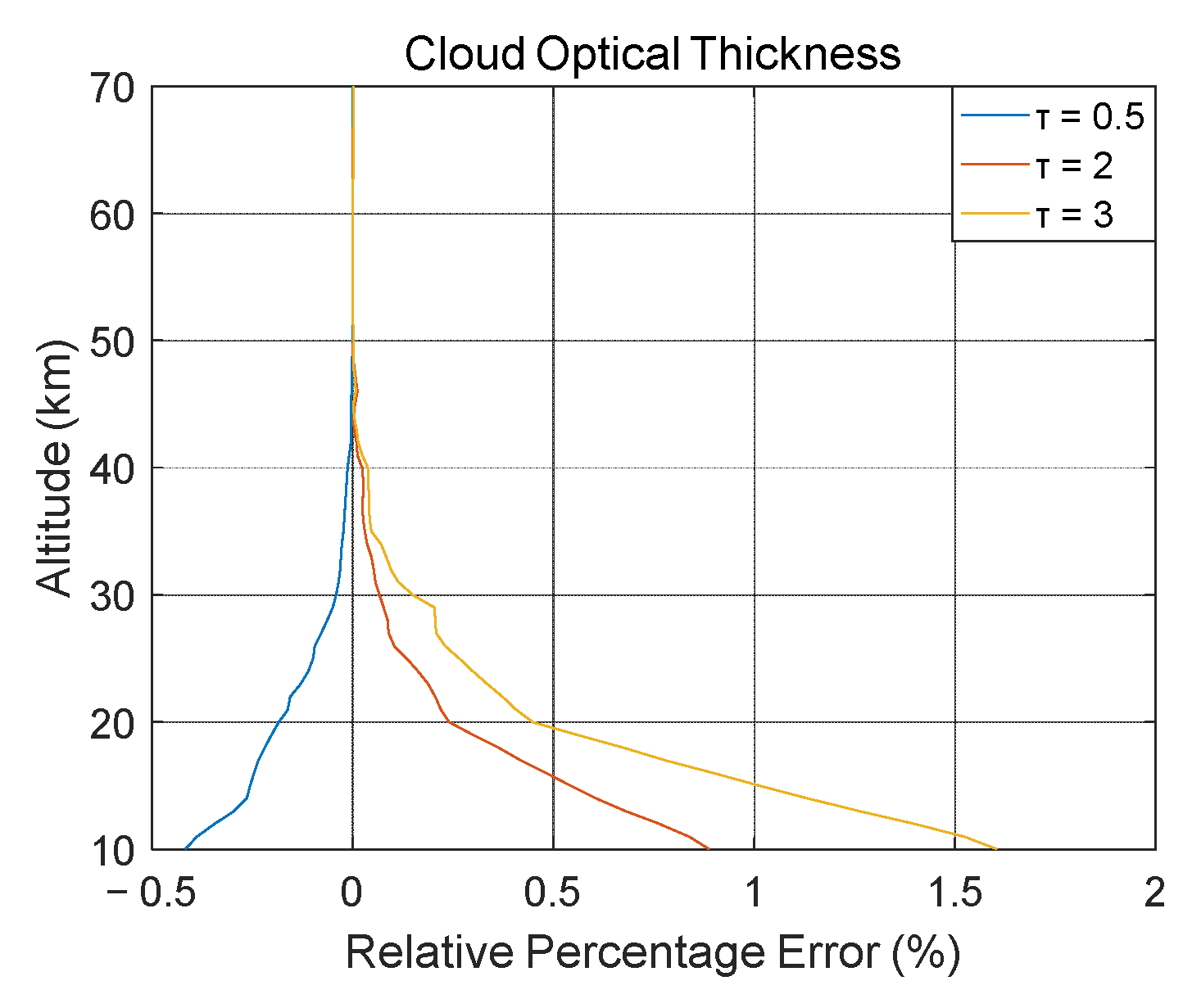
Cloud Optical Thickness

To investigate the sensitivity of cloud optical thickness (COT) to ozone retrievals, AS clouds with different COTs were used in the SCIATRAN model. COT uncertainties were adopted assuming $\mathsf{\tau }$ is 0.5, 2, and 3. The relative errors in the ozone retrieval between the correct and incorrect COTs are shown in Figure 9, where the impact of COT on ozone profile retrieval was primarily observed below 42 km and all errors were near zero above 42 km. Furthermore, the retrieved ozone concentration was higher when the COT increased and vice versa. When the COT was doubled, the error increased accordingly. The ozone retrieval error depended upon the optical depth of tropospheric clouds, because the reflected solar radiation of visible wavelengths varied with τ (i.e., thicker clouds optically reflect more sunlight). Therefore, the enhanced reflection caused by optically thick clouds led to an increase in limb radiance, which created a larger Chappuis triplet value and a smaller ozone concentration when retrieving profiles ignoring clouds.

Generally, the ozone retrieval error caused by the exclusion of clouds was attributable to the change in the limb signal from the presence of clouds in the atmosphere, which was notably similar to the disturbance of the vertical distribution of ozone; however, detailed information on cloud characteristics in real earth atmosphere observations was missing. Therefore, the error obtained from the retrieval of ozone profiles using cloudy and cloudless atmospheres in the RTM can be considered as that caused by ignoring clouds in the limb observations. Excluding the influence of clouds on the inversion of the ozone profile is essentially the same as ignoring the albedo deviation, all of which increases the reflected solar radiation. Therefore, if tropospheric clouds are ignored or modeled incorrectly, one way to reduce ozone retrieval errors is to use global daily reflectance maps (such as EP-TOMS) measurements and assume that CH is related to climate and latitude, although such methods will significantly reduce the retrieval speed of ozone profiles.

4.1.5. Total

The results are summarized in Tables S2–S11. The errors are the statistical results of the minimum error variable, where the minimum errors for each parameter were: −0.2 km for TH, +0.1 for albedo, AS cloud for CH, 200% for COT scaling, no aerosols for atmosphere, a comparison between 15° and 35°N for a priori profile, temperature and pressure profiles, and a comparison between 223 and 243 K cross-section values.

Table 1. Absolute values of the error (%) for retrieved ozone according to each error source. Parameter uncertainties were +0.1 for albedo, −200 m for TH, AS cloud for cloud height, 200% for cloud optical thickness (τ), no aerosols for atmosphere, 15°N vs. 35°N profile for bias, in addition to pressure and temperature, as well as a comparison between 223 and 243 K ozone cross-section values.

Para.	10 km	15 km	20 km	25 km	30 km	35 km	40 km	45 km	50 km	55 km	60 km	65 km	70 km	${\mathit{\sigma }}_{\mathit{t}\mathit{o}\mathit{t}}^{\mathit{A}\mathit{l}\mathit{t}}$	Rank
Bias	11.5	2.8	0.3	0.1	1.8	0.6	1.0	0.5	0.7	0.1	1.1	2.8	8.2	31.5	3
Alb.	2.8	1.8	1.0	0.6	0.4	0.3	0.2	0.0	0.0	0.0	0.0	0.0	0.0	7.1	5
Aer.	5.8	10.8	7.0	3.7	2.9	2.0	2.3	0.7	0.6	0.2	0.2	0.3	0.4	36.9	2
Press.	1.4	0.5	0.2	0.1	0.1	0.0	0.0	0.2	0.2	0.0	0.1	0.1	0.0	2.9	7
Temp.	0.0	0.6	0.1	0.1	0.0	0.0	0.0	0.4	0.0	0.3	0.3	0.2	0.1	2.1	8
T_ozone	0.5	0.5	0.4	0.4	0.6	0.8	1.4	1.4	0.7	0.3	0.2	0.0	0.0	7.2	4
TH	2.2	5.4	4.0	0.3	0.7	5.5	4.0	1.7	2.9	4.3	5.2	4.7	2.4	43.3	1
CH	1.6	0.5	0.8	0.4	0.0	0.1	0.1	0.0	0.0	0.0	0.0	0.0	0.0	3.5	6
τ	0.6	0.4	0.2	0.1	0.1	0.0	0.0	0.0	0.0	0.0	0.0	0.0	0.0	1.4	9

summarizes the error estimates for all sources (except random noise). The total error for each parameter in the entire retrieval range was ${\sigma }_{tot}^{Alt}={\sum }_{i=1}^N\left|{\sigma }^i\right|,N=13$ (where $N$ corresponds to the 13 specific altitudes). Table 1 shows that the main sources of ozone retrieval errors were the TH registration, stratospheric aerosols, and a priori ozone profile. The total error for surface albedo (+0.1) was almost the same as that of the ozone absorption cross-section (223 K), both equaling ~7%. Furthermore, the total error of the pressure profile was similar to that of the AS clouds (~3–3.5%), whereas that generated by the temperature profile was ~2%. Lastly, the total error of the COT was ~1.5%.

4.2. Impact of Solar Zenith Angle

Due to the similar latitudes and SZAs in each orbit, the estimation of various error sources for different solar zenith angles (30°:10°:90°) were investigated.

The ozone retrieval error caused by the a priori profile showed the same shape at altitudes under different SZAs (Figure S8). Figure 10a shows the distribution of errors generated by the a priori profiles as a function of SZA at 30 km, showing almost no difference in the relative errors for SZAs from 30° to 80°; however, once the SZA reached 90°, the relative error was noticeably larger, especially using a high latitude a priori profile. The errors display an obvious hierarchy in the different a priori profiles. Figure 10b shows the distribution of the average errors caused by surface albedos with SZAs, revealing that the errors caused by the same albedo deviation under different SZAs were the same at different altitudes, but the relative error decreased with increasing SZAs. This indicated that the uncertainty on ozone retrievals related to surface albedo were sensitive to SZAs.

Figure 10c shows the variation of ozone retrieval error with the solar zenith angle in the presence and absence of aerosols, indicating that aerosols are sensitive to SZAs, with errors growing as SZA increased, especially below 30 km. The distribution of ozone retrieval error with SZAs caused by aerosol extinction profiles with different scaling factors is shown in Figure 10d. The average error increased slightly with higher SZAs.

Figure 10e,f indicate the relative errors as a function of altitude caused by the pressure and temperature profiles under different SZAs, respectively. The error caused by the pressure profile changes slightly with the solar zenith angle, whereas the error at different heights varies with SZAs. In Figure 10f, the error shows little differences with changes in SZAs between 30° and 80°, however the error varied significantly from 23 to 43 km at SZAs of 90°.

The distribution of the ozone retrieval error with the SZAs at 30 km, caused by different ozone absorption cross-sections is shown in Figure 10g, where the error increased with an increase in the temperatures of the ozone absorption cross-section. However, the relative error hardly changed with SZAs, particularly between 30° and 80°. When the TH deviation was 200 m, the distribution of ozone retrieval error with the SZAs is shown in Figure 10h. Here, the sensitivity of the TH deviation to the SZA was small but changed at different altitudes.

Figure 10i,j indicate the distribution of the average errors of the three low clouds and high clouds at altitudes with SZAs. Below 42 km, at SZAs of <80°, the relative error increased with an increase in solar zenith angle, however the relative error decreased at an SZA of 90°. Notably, the influence of SZAs on 4–7 and 6–15 km clouds was similar to that of low clouds. The distribution of the average error caused by different COT with SZAs is shown in Figure 10k. Here, the error was found to be proportional to COT (i.e., the error increased steadily with the increase in cloud optical thickness), which is also sensitive to SZA.

To verify the sensitivity of the measurement vector to SZAs, the same random vector was used to retrieve the ozone profile at different SZAs. Figure 10l shows the noise errors for the different SZAs, where the random noise was insensitive to the SZA.

Figure 11 shows the average errors in the retrieval range for different SZAs, where the error sources most strongly dependent on the SZAs were aerosols, surface albedo, and clouds. Ozone retrieval errors caused by aerosols increased with an increase in SZA, while the error of the surface albedo decreased. The ozone retrieval error caused by clouds reached its maximum value at an SZA of 80°, whereas the a priori profile, TH, and temperature profile were only affected by SZAs of 90°. Among them, the error from the a priori profile and temperature increased at an SZA of 90°, while the error of tangent height decreased at an SZA of 90°. Notably, the ozone absorption cross-sections and pressure were largely unaffected by SZAs.

4.3. Differences between the Northern and Southern Hemispheres

Furthermore, NH and SH in the middle-latitude band (30–40°) were selected for further error estimation. The error estimate calculation was performed for 10 days during 2011, and included 165 NH in addition to 159 SH profiles.

Figure 12 shows the mean error and standard deviation of each hemisphere for all error sources, revealing that ozone retrieval errors caused by most error sources did not exhibit strong interhemispheric differences, with a notable exception for CH, which had a significantly greater impact on ozone retrieval in the NH. This may be related to the latitude change in the SCIAMACHY limb observation geometry, where the scattering angle in the NH was <~90°, while that in the SH was >~90°. Notably, the uncertainties for each parameter differed from those listed in Table 1. Table S12 summarizes the average errors of the sources at specific altitudes for both hemispheres.

The total systematic and random error of the NH and SH at different heights is listed in

Table 2. Total systematic and random uncertainties (%) for both hemispheres.

		10 km	15 km	20 km	25 km	30 km	35 km	40 km	45 km	50 km	55 km	60 km	65 km	70 km
Total systematic	NH	14.81	16.70	10.72	4.49	3.85	6.98	5.75	5.21	2.75	4.58	6.01	6.05	6.16
	SH	12.22	15.68	7.41	3.70	4.87	6.58	7.47	4.64	3.41	4.49	4.43	3.32	6.06
Total random	NH	4.66	1.97	0.06	0.03	2.43	0.55	3.74	2.20	0.84	1.97	0.12	0.66	0.85
	SH	5.04	1.31	0.15	0.07	2.45	0.49	3.70	2.23	0.87	2.07	0.16	0.69	0.77

. Figure 13a shows the average error profiles of each systematic error component in the NH, revealing the strongest contributions to the total systematic error at 15 km were aerosol ±15%, TH ±7%, CH ±2%, and surface albedo ±1.5%. In contrast, the total systematic error between 35 and 40 km was mainly attributed to the TH (±5%) and aerosols (±2%), whereas that between 40 and 50 km was primarily determined by the TH (±3%), a priori profile (±2.8%), and ozone absorption cross-section (±1.1%). Above 50 km, the total systematic error mainly originated from the TH (±4.8%) and the a priori profile (±2%). Figure 13b shows the total systematic and random errors of the two hemispheres. Below 26 km, the total systematic error in the NH was slightly larger than in the SH, likely due to the differences in error estimates of tropospheric AS clouds between the two hemispheres. Furthermore, there was almost no difference in the random error between the hemispheres, which was <5% of the entire retrieval range.

5. Discussion

The sensitivity analysis presented here shows results similar to previous studies [23,25,28,41]. For stratospheric aerosols, an error at 20 km (~7%) is obtained by ignoring aerosols, which decreases rapidly with increasing altitude (mainly affecting the stratosphere). In SAGE III, stratospheric aerosols were ignored, resulting in an error at ~20 km (6%) [41]. Furthermore, the aerosol extinction coefficient was reduced by 50%, resulting in an error of 3.7% at 20 km. This follows the results of Rahpoe et al. [25], in which an error of 40% aerosol disturbance at 20 km mid-latitudes NH was 2.9%. In the OSIRIS limb-scatter measurements, the aerosol profile was within 2-fold, with <5% error in the height range of 15–40 km [23], which also follows the present results (6%). For surface albedo, Wang et al., found that the maximum error at the lowest altitude did not exceed 2.5% for an albedo perturbation of 0.1 [28]. Here, calculating the +0.1 albedo perturbation generated a 2.45% error at 10 km. For a tropical albedo disturbance of 0.1, an error of 2% at 15 km was reported by Rahpoe et al. The third most common parameter used in this study was the TH. In SAGE III, an offset of 350 m was used, creating errors on the order of 5% and a peak error value of 12% at 15 km [41]. Rahpoe et al. [25] revealed an offset of 200 m, where the error at 19 km in mid-latitudes was ~5.2%, notably comparable to the findings of this study, with an error of ~5%.

Wang et al., derived an error of 7% at 20 km, when the offset was 0.25 km. The fourth most important source of error was cloud. The results suggest that clouds had a significant impact on the retrieval of ozone profiles below 40 km, whereas errors above 40 km could be ignored. Rahpoe et al., found that the errors in tropospheric clouds from 4 to 7 km were ~3% (tropical) and 5.5% (polar) at 10 km. This finding is consistent with our results (3.1%). von Savigny et al., concluded that tropospheric clouds (involving low, middle, and high clouds) had no significant effect on the retrieved ozone profile (the error increased from <2.5% at 15 km to <5% at 35 km), markedly different from the results here. In this study, the influence of clouds on ozone profile retrieval decreased with increasing altitude (the error of AS clouds decreased from < 1.8% at 10 km to < 0.2% at 35 km). Specifically, when the cloud layer was outside the field of view of the instrument (i.e., cloud top height was lower than the lowest retrieval height), the influence of cloud geometric thickness on ozone retrieval was small. The larger the COT, the greater the ozone retrieval error. Moreover, the influence of clouds on ozone retrieval was also affected by SZA. These results are consistent with those reported by Sonkaew et al. [22] and Wang et al. [28]. von Savigny et al., showed that the relative retrieval error did not exceed 1.0% from 15 to 40 km under the assumptions of T = 202 K, T = 241 K, and T = 273 K for the ozone cross-sections. This finding is notably consistent with ours (1.4%). The ozone retrieval error reported by Rahpoe et al., found that ±2 K uncertainty was <1% of all altitudes. The research here showed that the maximum relative error was ≤0.7%, with an uncertainty of ±5 K. The pressure uncertainty of Rahpoe et al., was ±1%, which produced an error of 1% for the retrieved ozone profile in most atmospheres. Here, the results showed that a 5% disturbance in the pressure profile produced a maximum error of ≤2%. Furthermore, the ozone retrieval errors caused by the a priori profiles at different latitudes were also performed in this study. This study showed that incorrect knowledge of the ozone profile both above and below the retrieval boundaries may result in an error of up ≤5.7% in the retrieved ozone profile, concurrent with the results of Roth et al., (6%) [21]. Furthermore, the measurement disturbance in this study followed a Gaussian distribution and was thus regarded a random error, leading to a retrieval error of the ozone profile ≤5%. Stray light and polarization effects can also contribute to the total error budget, and neglecting these additional parameters can lead to the underestimation of error.

6. Conclusions

The ozone profiles were retrieved from limb measurements under various conditions to evaluate the relative importance of the error sources. Experimental results revealed that the main sources of ozone retrieval error were TH registration, stratospheric aerosols, and a priori ozone profiles. The TH offset was the most significant problem throughout the entire retrieval range. For a TH offset of only 0.2 km, the total error generated at 13 specific altitudes was ~43% (Table 1), whereas aerosols had a significant impact on ozone retrieval <40 km. The total error in ozone retrieval between non-aerosols and background aerosols was ~37% (Table 1). The a priori profiles maintained larger error levels in the upper and lower retrieval boundaries, resulting from the fact that the ozone profile beyond its retrieval range can only change its size, and not its shape.

Our results provide insights into improving ozone retrieval results. For example, TH registration can be enhanced by improving the instrument pointing information (for example, by enhancing spacecraft attitude information using a spaceborne tracker). Although retrieving aerosol characteristics from the limb scatter radiance is challenging, a rough aerosol correction can significantly improve algorithm performance. Furthermore, using the ozone profiles of other satellites to establish an a priori database of monthly longitude and latitude grids can minimize the source of a priori errors. Notable secondary error sources included surface albedo and clouds. For surface albedo with a deviation of 0.1, the maximum error was ≤~3% at the lowest heights, whereas the influence of clouds on ozone retrieval occurred mainly in the stratosphere and ranged from ≤2% for low clouds and ≤5.5% for high clouds. Using global daily reflectance maps and assuming that CH is related to climate and latitude may further reduce errors. Notably, the retrieval error of ozone produced by the atmospheric pressure profile was larger than that for temperature. It was found that aerosols, surface albedo, and clouds were affected by SZA, with minor effects on a priori profiles, THs, and temperatures. Furthermore, the pressure and ozone absorption cross-sections were nearly unaffected by SZA.

The results of the sensitivity study on the retrieved ozone profile in NH and SH showed that the total systematic error below 20 km was mainly determined by aerosols, TH, clouds, and albedo; 30–50 km was most influenced by TH, aerosols, and a priori profiles, whereas >50 km was mainly determined by TH and a priori profiles. The total systematic error observed was 10–15% below 20 km, 2–6% between 20 and 35 km, 5–8% from 35 to 45 km, and 3–7.5% above 50 km. The overall shape of the total systematic error for NH and SH across the entire retrieval range was similar. The NH was slightly higher than the SH, which was attributed to the different scattering angles between the two locations. The contributions of the ozone absorption cross-section, atmospheric pressure, and temperature to the total systematic error can be ignored. In this study, random error was defined as the random disturbance of the measurement vector, where the disturbance is a random value with a Gaussian distribution. There was almost no difference in the total random error between the two hemispheres, with a controlled error within ±5%.

The results of the sensitivity analysis can be employed as total error limits for the validation and intercomparison activities of the SCIAMACHY ozone data, with other concurrent instruments. Although the retrieval errors varied slightly due to different retrieval algorithms and RTMs, the consistency of the ozone retrieval errors caused by the model parameters and the TH was relatively high here compared with other studies. Thus, the total error budget is critical, especially for long-term investigations of ozone behavior during climate change or for verification between different instrumental techniques.

References

1. Arosio, C.; Rozanov, A.; Malinina, E.; Eichmann, K.-U.; von Clarmann, T.; Burrows, J.P. Retrieval of ozone profiles from OMPS limb scattering observations. Atmos. Meas. Tech. 2018, 11, 2135–2149. [Google Scholar] [CrossRef]
2. Farman, J.C.; Gardiner, B.G.; Shanklin, J.D. Large Losses of Total Ozone in Antarctica Reveal Seasonal Clox/Nox Interaction. Nature 1985, 315, 207–210. [Google Scholar] [CrossRef]
3. Cicerone, R.J.; Stolarski, R.S.; Walters, S. Stratospheric Ozone Destruction by Man-Made Chlorofluoromethanes. Science 1974, 185, 1165–1167. [Google Scholar] [CrossRef] [PubMed]
4. Solomon, S.; Ivy, D.J.; Kinnison, D.; Mills, M.J.; Neely, R.R.; Schmidt, A. Emergence of healing in the Antarctic ozone layer. Science 2016, 353, 269–274. [Google Scholar] [CrossRef]
5. Li, F.; Stolarski, R.S.; Newman, P.A. Stratospheric ozone in the post-CFC era. Atmos. Chem. Phys. 2009, 9, 2207–2213. [Google Scholar] [CrossRef]
6. Hassler, B.; Petropavlovskikh, I.; Staehelin, J.; August, T.; Bhartia, P.K.; Clerbaux, C.; Degenstein, D.; De Maziere, M.; Dinelli, B.M.; Dudhia, A.; et al. Past changes in the vertical distribution of ozone—Part 1: Measurement techniques, uncertainties and availability. Atmos. Meas. Tech. 2014, 7, 1395–1427. [Google Scholar] [CrossRef]
7. Van Peet, J.C.A.; van der, A.R.J.; de Laat, A.T.J.; Tuinder, O.N.E.; König-Langlo, G.; Wittig, J. Height resolved ozone hole structure as observed by the Global Ozone Monitoring Experiment-2. Geophys. Res. Lett. 2009, 36, 269–271. [Google Scholar] [CrossRef]
8. Huang, F.; Liu, N.; Zhao, M.-X.; Wang, S.; Huang, Y. Vertical ozone profiles deduced from measurements of SBUS on FY-3 satellite. Chin. Sci. Bull. 2010, 55, 943–948. [Google Scholar] [CrossRef]
9. Levelt, P.F.; Van den Oord, G.H.J.; Dobber, M.R.; Malkki, A.; Visser, H.; de Vries, J.; Stammes, P.; Lundell, J.O.V.; Saari, H. The Ozone Monitoring Instrument. IEEE Trans. Geosci. Remote Sens. 2006, 44, 1093–1101. [Google Scholar] [CrossRef]
10. Qian, Y.; Luo, Y.; Si, F.; Zhou, H.; Yang, T.; Yang, D.; Xi, L. Total Ozone Columns from the Environmental Trace Gases Monitoring Instrument (EMI) Using the DOAS Method. Remote Sens. 2021, 13, 2098. [Google Scholar] [CrossRef]
11. Bertaux, J.L.; Kyrölä, E.; Fussen, D.; Hauchecorne, A.; Dalaudier, F.; Sofieva, V.; Tamminen, J.; Vanhellemont, F.; D’Andon, O.F.; Barrot, G.; et al. Global ozone monitoring by occultation of stars: An overview of GOMOS measurements on ENVISAT. Atmos. Chem. Phys. 2010, 10, 12091–12148. [Google Scholar] [CrossRef]
12. Chateauneuf, F.J.; Fortin, S.Y.; Buijs, H.L.; Soucy, M.-A.A. On-orbit performance of the ACE-FTS instrument. Earth Obs. Syst. Ix 2004, 5542, 166–175. [Google Scholar]
13. Adams, C.; Bourassa, A.E.; Bathgate, A.F.; McLinden, C.A.; Lloyd, N.D.; Roth, C.Z.; Llewellyn, E.J.; Zawodny, J.M.; Flittner, D.E.; Manney, G.L.; et al. Characterization of Odin-OSIRIS ozone profiles with the SAGE II dataset. Atmos. Meas. Tech. 2013, 6, 1447–1459. [Google Scholar] [CrossRef]
14. McPeters, R.D.; Janz, S.J.; Hilsenrath, E.; Brown, T.L.; Flittner, D.E.; Heath, D.F. The retrieval of O-3 profiles from limb scatter measurements: Results from the Shuttle Ozone Limb Sounding Experiment. Geophys. Res. Lett. 2000, 27, 2597–2600. [Google Scholar] [CrossRef]
15. Llewellyn, E.; Lloyd, N.D.; Degenstein, D.A.; Gattinger, R.L.; Petelina, S.V.; Bourassa, A.E.; Wiensz, J.T.; Ivanov, E.V.; McDade, I.C.; Solheim, B.H.; et al. The OSIRIS instrument on the Odin spacecraft. Can. J. Phys. 2004, 82, 411–422. [Google Scholar] [CrossRef]
16. Bovensmann, H.; Burrows, J.P.; Buchwitz, M.; Frerick, J.; Noël, S.; Rozanov, V.V.; Chance, K.V.; Goede, A.P.H. SCIAMACHY: Mission objectives and measurement modes. J. Atmos. Sci. 1999, 56, 127–150. [Google Scholar] [CrossRef]
17. Rault, D.F. Ozone, NO2 and aerosol retrieval from SAGE III limb scatter measurements. Remote Sens. Clouds Atmos. Ix 2004, 5571, 205–216. [Google Scholar]
18. Rault, D.F.; Loughman, R.P. The OMPS Limb Profiler Environmental Data Record Algorithm Theoretical Basis Document and Expected Performance. IEEE Trans. Geosci. Remote Sens. 2013, 51, 2505–2527. [Google Scholar] [CrossRef]
19. von Savigny, C.; Haley, C.S.; Sioris, C.E.; McDade, I.C.; Llewellyn, E.J.; Degenstein, D.; Evans, W.F.J.; Gattinger, R.L.; Griffioen, E.; Kyrölä, E.; et al. Stratospheric ozone profiles retrieved from limb scattered sunlight radiance spectra measured by the OSIRIS instrument on the Odin satellite. Geophys. Res. Lett. 2003, 30, 107–218. [Google Scholar] [CrossRef]
20. Loughman, R.P.; Flittner, D.E.; Herman, B.M.; Bhartia, P.K.; Hilsenrath, E.; McPeters, R.D. Description and sensitivity analysis of a limb scattering ozone retrieval algorithm. J. Geophys. Res. Atmos. 2005, 110. [Google Scholar] [CrossRef]
21. Roth, C.; Degenstein, D.; Bourassa, A.; Llewellyn, E. The retrieval of vertical profiles of the ozone number density using Chappuis band absorption information and a multiplicative algebraic reconstruction technique. Can. J. Phys. 2007, 85, 1225–1243. [Google Scholar] [CrossRef]
22. Sonkaew, T.; Rozanov, V.V.; Von Savigny, C.; Rozanov, A.; Bovensmann, H.; Burrows, J.P. Cloud sensitivity studies for stratospheric and lower mesospheric ozone profile retrievals from measurements of limb-scattered solar radiation. Atmos. Meas. Tech. 2009, 2, 653–678. [Google Scholar] [CrossRef]
23. von Savigny, C.; McDade, I.C.; Griffioen, E.; Haley, C.S.; Sioris, C.E.; Llewellyn, E.J. Sensitivity studies and first validation of stratospheric ozone profile retrievals from Odin/OSIRIS observations of limb-scattered solar radiation. Can. J. Phys. 2005, 83, 957–972. [Google Scholar] [CrossRef]
24. Wang, Z.; Chen, S.; Jin, L.; Yang, C. Ozone profiles retrieval from SCIAMACHY Chappuis-Wulf limb scattered spectra using MART. Sci. China-Phys. Mech. Astron. 2011, 54, 273–280. [Google Scholar] [CrossRef]
25. Rahpoe, N.; von Savigny, C.; Weber, M.; Rozanov, A.; Bovensmann, H.; Burrows, J.P. Error budget analysis of SCIAMACHY limb ozone profile retrievals using the SCIATRAN model. Atmos. Meas. Tech. 2013, 6, 2825–2837. [Google Scholar] [CrossRef]
26. Zhu, F.; Si, F.Q.; Zhan, K. Research on Ozone Profiles Retrieval Using Chappuis-Wulf Band Absorption Information from Limb Scattered Measurement. Acta Opt. Sin. 2021, 41, 39–48. [Google Scholar]
27. von Clarmann, T.; Degenstein, D.A.; Livesey, N.J.; Bender, S.; Braverman, A.; Butz, A.; Compernolle, S.; Damadeo, R.; Dueck, S.; Eriksson, P.; et al. Overview: Estimating and reporting uncertainties in remotely sensed atmospheric composition and temperature. Atmos. Meas. Tech. 2020, 13, 4393–4436. [Google Scholar] [CrossRef]
28. Wang, Z.J. Study on retrieval of atmospheric trace gas concentrations from satellite based limb radiance. In Earth Exploration Science and Technology; Jilin University: Changchun, China, 2011; p. 197. [Google Scholar]
29. Degenstein, D.A.; Bourassa, A.E.; Roth, C.Z.; Llewellyn, E.J. Limb scatter ozone retrieval from 10 to 60 km using a multiplicative algebraic reconstruction technique. Atmos. Chem. Phys. 2009, 9, 6521–6529. [Google Scholar] [CrossRef]
30. Flittner, D.E.; Bhartia, P.K.; Herman, B.M. O3 profiles retrieved from limb scatter measurements: Theory. Geophys. Res. Lett. 2000, 27, 2601–2604. [Google Scholar] [CrossRef]
31. Chahine, M.T. General Relaxation Method for Inverse Solution of Full Radiative Transfer Equation. J. Atmos. Sci. 1972, 29, 741–747. [Google Scholar] [CrossRef]
32. Roth, C.Z. Atmospheric Ozone Retrieval using Radiance Measurements from the Chappuis and Hartley-Huggins Absorption Bands. In Physics and Engineering Physics; University of Saskatchewan: Saskatoon, SK, Canada, 2007. [Google Scholar]
33. Rozanov, V.; Dinter, T.; Wolanin, A.; Bracher, A.; Burrows, J.P. Radiative transfer modeling through terrestrial atmosphere and ocean accounting for inelastic processes: Software package SCIATRAN. J. Quant. Spectrosc. Radiat. Transf. 2017, 194, 65–85. [Google Scholar] [CrossRef]
34. Rozanov, V.V.; Diebel, D.; Spurr, R.J.D.; Burrows, J.P. GOMETRAN: A radiative transfer model for the satellite project GOME, the plane-parallel version. J. Geophys. Res. Atmos. 1997, 102, 16683–16695. [Google Scholar] [CrossRef]
35. Rozanov, A.; Rozanov, V.; Buchwitz, M.; Kokhanovsky, A.; Burrows, J.P. SCIATRAN 2.0—A new radiative transfer model for geophysical applications in the 175–2400 nm spectral region. Adv. Space Res. 2005, 36, 1015–1019. [Google Scholar] [CrossRef]
36. Rodgers, C.D. Retrieval of Atmospheric-Temperature and Composition from Remote Measurements of Thermal-Radiation. Rev. Geophys. 1976, 14, 609–624. [Google Scholar] [CrossRef]
37. Puliafito, E.; Bevilacqua, R.; Olivero, J.; Degenhardt, W. Retrieval Error Comparison for Several Inversion Techniques Used in Limb-Scanning Millimeter-Wave Spectroscopy. J. Geophys. Res. Atmos. 1995, 100, 14257–14267. [Google Scholar] [CrossRef]
38. Bourassa, A.E.; Degenstein, D.A.; Gattinger, R.L.; Llewellyn, E.J. Stratospheric aerosol retrieval with optical spectrograph and infrared imaging system limb scatter measurements. J. Geophys. Res. Atmos. 2007, 112. [Google Scholar] [CrossRef]
39. Rodgers, C.D. Inverse Methods for Atmospheric Sounding: Theory and Practice. Series on Atmospheric, Oceanic and Planetary Physics Volume 2; World Scientific: Singapore, 2000; p. 238. [Google Scholar]
40. McLinden, C.A.; McConnell, J.C.; McElroy, C.T.; Griffioen, E. Observations of stratospheric aerosol using CPFM polarized limb radiances. J. Atmos. Sci. 1999, 56, 233–240. [Google Scholar] [CrossRef]
41. Rault, D.F.; Taha, G. Validation of ozone profiles retrieved from Stratospheric Aerosol and Gas Experiment III limb scatter measurements. J. Geophys. Res. Atmos. 2007, 112. [Google Scholar] [CrossRef]
Figure 1. (a) Latitude distribution of SZAs on 14 April (blue ‘+’), 14 July (red ‘o’), 14 October (green ‘*’), and 14 December (purple ‘·’) in 2011; (b) latitude distribution of the SZAs for orbit 50200 (blue ‘o’), 50201 (red ‘·’), and 50202 (green ‘*’) on 5 October 2011.
Remotesensing 14 03954 g001
Figure 2. A sample of SCIAMACHY limb radiance profiles on orbit 49886 on 13 September 2011: (a) limb radiance profiles at different latitudes and corresponding SZAs in the northern hemisphere; (b) limb radiance profiles of the northern and southern hemispheres at the same latitudes and corresponding SZAs.
Remotesensing 14 03954 g002
Figure 3. Relative errors attributed to a priori profiles at different latitudes.
Remotesensing 14 03954 g003
Figure 4. Relative percentage error of SCIAMACHY limb ozone profiles simulated for correct and incorrect values in parameter settings. (a) Albedo; (b) aerosol extinction profile.
Remotesensing 14 03954 g004
Figure 5. Ozone retrieval error caused by neutral density. (a) Pressure profiles at different latitudes; (b) temperature profiles at different latitudes.
Remotesensing 14 03954 g005
Figure 6. Relative errors of ozone concentration retrieved from ozone absorption cross sections at different temperatures.
Remotesensing 14 03954 g006
Figure 7. Relative percentage error. (a) Different tangent height deviations; (b) random noise.
Remotesensing 14 03954 g007
Figure 8. Relative errors between cloud and no cloud cover. (a) Low cloud coverage; (b) high clouds.
Remotesensing 14 03954 g008
Figure 9. Relative errors of different cloud optical thicknesses.
Remotesensing 14 03954 g009
Figure 10. Distribution of the ozone retrieval errors for error sources with SZAs. (a) A priori profiles; (b) surface albedo; (c) aerosol; (d) aerosol extinction coefficient; (e) pressure; (f) temperature; (g) temperature of ozone absorption cross section; (h) tangent height; (i) low cloud; (j) high cloud; (k) cloud optical thickness; (l) random noise.
Remotesensing 14 03954 g010aRemotesensing 14 03954 g010b
Figure 11. Average errors (%) of retrieved ozone from an altitude between 10 and 70 km at different SZAs, for the same parameters as in Table 1. (a) Bias, aerosol and TH; (b) albedo, pressure, temperature, ozone absorption cross section, CH and COT.
Remotesensing 14 03954 g011
Figure 12. Average error profiles from an altitude of 10 to 70 km for the NH and SH. The uncertainties for each parameter were +0.1 for albedo, −50% for a priori ozone profile scaling, −5% for pressure, −5 K for temperature, and +200 m for tangent height, a comparison between 223 and 243 K experimental cross-section values, AS clouds, −50% for cloud optical thickness scaling, and no aerosols for atmosphere. Standard deviations are shown in the shaded regions.
Remotesensing 14 03954 g012
Figure 13. (a) Average error profiles for each systematic error component in the NH, using the same parameters as in Figure 12; (b) total systematic and random errors in both hemispheres.
Remotesensing 14 03954 g013