Article

Sentinel-2 Poplar Index for Operational Mapping of Poplar Plantations over Large Areas

1
University of Toulouse, INRAE, UMR DYNAFOR, 31320 Castanet-Tolosan, France
2
Conseil National du Peuplier, 75116 Paris, France
3
Centre National de la Propriété Forestière, Institut pour le Développement Forestier, 33075 Bordeaux, France
*
Author to whom correspondence should be addressed.
Remote Sens. 2022, 14(16), 3975; https://doi.org/10.3390/rs14163975
Submission received: 30 June 2022 / Revised: 25 July 2022 / Accepted: 12 August 2022 / Published: 16 August 2022

Abstract

:
Poplar (Populus spp.) is a fast-growing tree planted to meet the growing global demand for wood products. In France, the country with the largest area planted with poplar in Europe, accurate and up-to-date maps of its spatial distribution are not available at the national scale. This makes it difficult to estimate the extent and location of the poplar resource and calls for the development of a robust and timely stable approach for mapping large areas in order to ensure efficient monitoring. In this study, we investigate the potential of the Sentinel-2 time series to map the diversity of poplar plantations at the French countrywide scale. By comparing multiple configurations of spectral features based on spectral bands and indices over two years (2017 and 2018), we identify the optimal spectral regions with their respective time periods to distinguish poplar plantations from other deciduous species. We also define a novel poplar detection index (PI) with four variants that combine the best discriminative spectral bands. The results highlight the relevance of SWIR followed by red edge regions, mainly in the growing season, to accurately detect poplar plantations, reflecting the sensitivity of poplar trees to water content throughout their phenological cycle. The best performances with stable results were obtained with the PI 2 poplar index combining the B5, B11, and B12 spectral bands. The PI 2 index was validated over two years with an average producer’s accuracy of 92% in 2017 and 95% in 2018. This new index was used to produce the national map of poplar plantations in 2018. This study provides an operational approach for monitoring the poplar resource over large areas for forest managers.

1. Introduction

Timely and accurate mapping of the distribution and composition of forest stands is essential for both forest management and biodiversity assessment [1]. According to the most recent Global Forest Resources Assessment by the Food and Agriculture Organization (FAO), the total area of the world’s forests is 4.06 billion hectares, of which 93% is naturally regenerating forests and 7% is planted forests [2]. While the area of naturally generating forests has been decreasing since 1990, planted forests have increased by about 123 million hectares over the same period, indirectly compensating for some of the area lost through deforestation [3]. The importance of planted forests has continued to increase as wood has become an increasingly crucial raw material for industry and an attractive source of bioenergy. In the last two decades, short-rotation coppice (SRC) plantations such as poplar have been among the most important fast-growing planted tree species. Poplar plantations are widely distributed throughout the world and mainly cultivated in China, western Europe, and North America for their high-quality timber, high growth rate, and short rotation cycle of about 20 years [4].
In France, poplar plantations are an important economic resource mainly exploited to satisfy the growing demand for wood. According to the latest report by the International Poplar Commission, the surface area of poplar plantations in France was estimated at 0.2 million hectares [4] (i.e., one tenth of the national forest). These area estimates come from forest databases, cadastral surveys, or statistical forest inventories, but have never been established synchronously using a homogeneous approach throughout the country, and the extent and location of the plantations are generally not reported. Consequently, it is difficult to accurately estimate the surface area of these plantations and regularly monitor the dynamics of the poplar resource.
Different remote sensing techniques have been developed to map forest stands [5] by identifying forest cover and the dominant leaf type (e.g., broadleaf or coniferous) [6,7] and even go as far as characterising the composition of forest tree species [8,9,10,11].
Some studies have focussed more specifically on mapping forest plantations [12] notably rubber [13,14,15], palm oil [16,17], and eucalyptus [18,19,20], as well as acacia [21]. Although significant efforts have been made to identify some natural poplars (mainly European aspen, Populus tremula L. and quaking aspen, Populus tremuloides Michx.) [22,23,24], little effort has been devoted to hybrid poplar plantations in temperate regions (Populus deltoides × Populus nigra; Populus deltoides × Populus trichocarpa; Populus trichocarpa × Populus maximowiczii), including the many different cultivars used and stand development stages [25,26,27,28,29].
Chardenon and Flouzat [25] tested the capabilities of Landsat-2 imagery to classify poplar stands in France (in the Garonne River plain) and Italy (in the Pô valley), with different canopy cover rates related to stand age. These authors achieved only limited success using a single image acquired in May, July, and October 1972 and in June, July, and September 1975. Discrimination was improved using a bitemporal classification based on images acquired in June and September 1975, with 49.4% accuracy for young plantations (cover rate < 25%) and 80.8% for older (cover rate > 25%). Young plantations were difficult to identify due to the presence of herbaceous understory vegetation. The authors also remarked on the inadequacy of the Landsat-2 spatial resolution (80 m) to identify many small poplar stands (<1 ha). In another study, Borry et al. [26] concluded that the discrimination of poplar stands at different development stages is possible using one single image acquired in the full growing season. Their results, in contrast to those of Chardenon and Flouzat [25], were obtained with SPOT-1 HRV (20 m spatial resolution) and Landsat-5 TM (30 m) images. Based on a per-field classification, young stands were classified with 80–94% accuracy, middle age stands with 45–77% accuracy, and older with 46–74% accuracy, depending on the spectral band and the date selected. The authors found that combining several dates did not improve the discrimination. The stand sizes were relatively small, ranging from 0.5 to 2 hectares, with different types of understorey vegetation (herbaceous layer, dense or scattered shrubs). Object-based classification of poplar plantations using very-high-spatial-resolution (Ikonos and Quickbird) imagery was also investigated by Grignetti et al. [27]. Overall accuracy ranging from 74% to 82% was obtained but with very unreliable identification in the case of new plantations (<3 years old), as in [29]. Other interesting approaches at the tree level and stand level are reported in [24] based on LiDAR data, airborne photogrammetry, and multispectral and hyperspectral imaging. However, most concern aspen trees in natural contexts, especially in boreal forest landscapes.
The above-mentioned studies produced contrasting results concerning the ability to produce accurate maps of poplar plantations in various management contexts. Differences in the levels of reflectance between plantations of poplar species and other tree species in natural forests were not examined, nor was the possible identification of specific wavelength regions or spectral indices for poplar discrimination. In addition, it is not clear whether integrating the temporal dimension in the classification procedure is useful for poplar, even though seasonal variations in vegetation (i.e., phenology) could improve performances [30,31]. Moreover, previous studies were limited to local areas, making it difficult to evaluate if identical findings would be obtained for larger areas.
In this study, we investigated the automatic classification of all hybrid poplar plantations at the French national scale using optical Sentinel-2 (S2) time series. We hypothesised that time-series data would enable better classification than mono-temporal images. S2 data has been recently explored to identify poplar plantations [29]. However, the study was conducted on a limited number of S2 image tiles in Northern Italy and for plantations mainly composed of the I214 (P. × euroamericana) cultivar. Here, our main objective was to define a generic methodological approach to map the wide range of hybrid poplar plantations in an operational context and to identify the key spectral features for poplar recognition. After a preliminary spectral analysis based on visual interpretation, we used a feature selection technique to select optimal bands and spectral indices at specific dates for poplar discrimination. We also defined a new S2 poplar detection index (PI) with four variants to improve the classification. We evaluated its stability over two years on three contrasting poplar sites at different stand development stages. The best version of PI was then used to produce the map of poplar plantations at the national scale. This study provides a practical approach for monitoring the poplar resource in the near future by plantation managers.

2. Materials

2.1. Satellite Data

In collaboration with forest partners, we chose three S2 image tiles (each covering 100 km × 100 km) to conduct the analysis. These tiles are located in the north-east, centre, and south-west of France (Figure 1). They cover the most contrasting poplar sites in terms of diversity related to silvicultural practices, types of cultivars planted, soil, and climate conditions. The 31UEQ tile is located in the degraded oceanic climate region of the north and centre plains. The 30TYT tile is located in the altered oceanic climate, while the 31TCJ is characterised by the southwest basin climate with possible summer drought [32].
Two years, 2017 and 2018, were considered independently to check the concordance of the results between years. All available S2 images of the three tiles and for the two years were downloaded from the French THEIA Land Data Center, including both S2A and S2B data. Top of atmosphere (TOA) surface reflectance products (level 2A) were used, meaning the data have been orthorectified and corrected for topographic and atmospheric effects. Images were pre-processed by THEIA with the MAJA platform, and a cloud mask was provided with each acquisition [34].
We only selected the 10 m and 20 m spectral bands of the two S2 satellites, the other bands (1, 9, and 10) at 60 m spatial resolution being dedicated to atmospheric correction and cloud screening. At 10 m, four spectral bands are available: blue (B2), green (B3), red (B4), and near infrared (B8). At 20 m, six spectral bands are provided: red edge (B5, B6, B7), near infrared (8A), and short-wave infrared (B11, B12). The precise characteristics of the S2 spectral bands are summarised in Table 1.
Because of specific sensor constraints (e.g., different relative orbits) or the cloud cover, the acquisitions of one year are non-synchronous in the three study tiles. Therefore, for each S2 time series of the same year, all the images were resampled to 10 m spatial resolution with nearest-neighbour resampling and with the same 10-day time step for all tiles. While performing the temporal resampling, missing data (i.e., pixels that were invalid due to clouds or cloud shadows) were filled using a multi-temporal linear interpolation. This involved replacing each cloudy and shady pixel (detected in the cloud mask) with an interpolated value derived from the nearest valid pixels in the times series [35]. The resulting gap-filled image time series comprise 340 features in 2017 (34 dates × 10 spectral bands) and 360 features in 2018 (36 dates × 10 spectral bands).
The resampled dates are detailed in Appendix A.

2.2. Reference Data

Reference polygons for training and testing were drawn in the three S2 tiles from the latest version of the French National Forest Inventory (NFI) spatial database (BD Forêt® IGN, v.2) produced by the national mapping agency (IGN). This database provides a vector map of forest stands (polygons) with a minimum area of 0.5 hectares. The composition of each stand was obtained by interpreting aerial stereo images complemented by field surveys. This map was produced progressively, district by district, starting in 2007. National coverage was completed in 2018. We only considered classes of deciduous species in this forest map, including poplar plantations. Coniferous species were excluded. Pure and mixed stands of deciduous species were retained. While pure stands consist of polygons covered by 75% of a single dominant deciduous species, mixed stands of predominant deciduous have only 50% to 75% coverage, with no information about the species. In the database, poplar plantation polygons are always referred to as pure stands.
Since there is a time lag between the year when the forest database was made available (between 2007 and 2018, depending on the district) and the year of acquisition of the S2 time series, all poplar polygons for both 2017 and 2018 were checked through photo interpretation, each of them by three different experts. This step ensured up-to-date references as poplar stands may change over time due to their short rotation cycle. The photo interpretation was based on high-resolution (HR) aerial orthophotos from IGN dating from 2016, 2018, or 2019, depending on the district, but also from Google Earth and Google Street View, paying attention to the date of the available images. Poplar plantations are easy to recognise in HR images because of the regular spacing of trees, the stand homogeneity, and the ovoid shape of the tree tops [36]. In each tile, we selected references of various stand ages (from 3 to 20 years and sometimes more in tile 31UEQ, some plantations being abandoned), but very young plantations (<3 years approximately) were excluded because of their limited canopy cover rate and the difficulty involved in identifying them accurately through photo interpretation. We also selected various cultivars in each tile, with a total of at least 30 cultivars for the three tiles. This number was estimated by forest partners based on the past and current list of cultivars eligible for state subsidies, but their respective proportions in the reference dataset is unknown (the cultivars not being available in the forest database).
A set of reference poplar polygons from the southwestern tile (31TCJ) was validated in the field by forest partners. Out of a total of 230 photo-interpreted polygons, two were eucalyptus plantations, representing less than 1% misidentification. As a separate test, a set of 85 field-checked polygons was also used to study the effect of the stage of development of the poplar stand on the detection by S2 data. Reference pixels for the other deciduous species were drawn directly from the forest database, without checking or updating. All of them were considered as non-poplar class after classification.
A data-cleaning step was applied to all the pixels included in the reference polygons of the three S2 tiles to eliminate outliers arising from undetected clouds in the time series (i.e., for which no gap-filling had been performed) or from pixels that differ significantly from their membership class (e.g., urban pixels or pixels showing bare soil in pure stands). The outlier detection procedure followed the 1.5 interquartile range rule (1.5 IQR), which considers values outside the interval [ Q 1 1.5 I Q R ; Q 3 + 1.5 I Q R ] as outliers, where Q1 and Q3 denote the first and third quartiles, respectively. The outlier detection procedure first consisted in eliminating all pixels outside the predefined interval in each band of the time series and for each tree species class separately. Thereafter, and proceeding by class, only the valid pixels common to all bands in the time series were retained. In this way, if pixels were detected as outliers in only one band, they were automatically removed from the sample set. Finally, the number of samples per class was set so that the smallest class was fully sampled.
The total number of sampled pixels in each tile and for each year, after removal of the outliers, is listed in Table 2. The sample size for poplars varied between 2500 and 7700 pixels in 2017 and between 3200 and 5000 in 2018. The difference between the number of samples in 2017 and 2018 is due to the fact there were more outliers in 2018. The black locust tree class was removed from tile 31UEQ in 2018 because the majority of its samples were identified as outliers and the number of remaining pixels was too small to be considered as a specific class in the learning process.

3. Methods

We used a statistical approach based on the sequential forward floating selection (SFFS) algorithm to measure the importance of spectral features and to select the best subset of bands and spectral indices for the classification of poplar stands among the other tree species. The analysis was conducted in three steps. First, we detected the most important spectral features and time periods for poplar identification using a combination of all S2 spectral bands and acquisitions of the time series (Figure 2a). This was carried out separately for 2017 and 2018. Then, based on these results, we identified a set of existing potentially discriminative spectral indices. We also defined a new S2 poplar detection index (PI) with four variants to improve the classification. We selected features from this set of data to identify the most relevant combination of spectral indices in terms of poplar recognition (Figure 2b). Finally, we evaluated each spectral feature independently using all available dates in each time series (Figure 2c,d) and compared the classification performances with those of the previous subsets of features (combination of spectral bands or indices). The best feature subset with the most stable performance for the two years was used to produce the map of poplar plantations at the national scale.

3.1. Feature Selection with SFFS

Several techniques have been proposed to address the problem of identifying a subset of relevant variables (features) in a large input dataset [37,38]. In remote sensing, this helps to identify specific spectral features and periods related to the classes of interest, before examining the possible origins and before trying to understand the underlying physical processes. This also reduces the effect of the curse of dimensionality (or Hughes phenomenon [39]), which appears with too many features and has a negative impact on classification performance [31]. In addition, it eliminates redundant or noisy features and reduces the computation time required to process the data.
In this study, we used SFFS, a wrapper-based feature selection algorithm [40]. SFFS is a standard method that has already been shown to provide a good trade-off between computation time and efficiency [41,42]. Compared to feature extraction techniques that rely on data transformation methods (such as principal component analysis) independently of the classification, wrapper-based approaches perform feature selection using a classification algorithm to evaluate subsets, the predictive performance being the objective function [38].
SFFS is a bottom-up search procedure that selects an optimal subset of features, starting from an empty set, and at each iteration, adds the most important feature (i.e., the one with the highest value for the objective function) to the pool of selected features. SFFS is a more flexible version of the initial sequential forward selection (SFS) method, in which individual features are permanently conserved after selection, with no backtracking. The floating search approach overcomes the so-called nesting effect by performing a backward selection after each SFS step to conditionally exclude one of the previously selected features, thus avoiding a local minimum [40]. The feature is removed if a subset of the same size achieves better accuracy according to a given performance criterion. In this way, it is possible to rectify the inclusion of previous features and to replace them with new better features in order to converge towards the optimal solution. The iteration continues until the required number of features is added or the expected performance is reached.
This method was used to identify the most relevant subsets that offer the best classification performance in each feature space. This was carried out until ten features were included in the subset, to limit computation time, and after checking that the addition of extra features did not improve the classification performance. This selection was applied for both multi-feature and single-feature SFFS configurations (Figure 2). In the so-called single-feature SFFS configuration, the spectral band or index remains unique, but several dates can be selected (with a maximum of 10).

3.2. Sample Selection, Classification and Comparison of Performances

A total of 512 reference polygons (forest stands) were available in the dataset, with 254 polygons in image tile 31TCJ, 155 in tile 31UEQ, and 103 in tile 30TYT. After pooling, reference polygons were randomly separated into 50% for training and 50% for testing. The S2 pixels (10 m square) were then sampled in each subset of polygons, and feature values were extracted from each gap-filled time series in 2017 and 2018. To ensure the balance of classes in each tile, training and testing pixels were selected from reference polygons using stratified random sampling of equal size for each class. Training and testing pixels were collected from spatially disjoint reference polygons in order to limit spatial autocorrelation effects [43].
SFFS was computed only on the training set (50% of the samples) with five-fold cross-validation. Each model with the best subset of ten features (one for each SFFS configuration) was then evaluated on the independent test set (50% of the remaining samples).
We used random forest (RF) as a supervised classification algorithm [44]. Tuning the hyperparameters, including the number of decision trees, the maximum depth of the trees, and the number of features considered by each tree when splitting a node, was based on a grid-search strategy and five-fold cross-validation. The number of trees tested ranged from 10 to 150, with a step of 10. The values tested for trees depth included the maximum possible value that expands the tree nodes until all the leaves become pure, as well as intermediate values between 5 and 50, with an interval of 10. As recommended, the number of features to split each node was set to the square root of the total number of input variables [44,45] in addition to a range of values between 1 to 20, with a step of 2.
Classification performance was assessed in terms of producer’s accuracy (PA), also known as recall, for the poplar class. PA was used as the objective function (i.e., performance predictor) in SFFS. It is a non-prevalence-dependent performance measure that, for a given class, corresponds to the number of correctly identified samples among all reference samples assigned to that class. Confusion matrix with user’s accuracy (UA) and F-score (harmonic mean of UA and PA) were also computed. As recommended by Foody [46], we deliberately disregarded the kappa metric.
The performances of the best models (i.e., those built with the optimal feature subsets derived for each configuration in Figure 2) were compared using McNemar’s statistical test [47], which is a non-parametric alternative to the T-test to examine the statistical significance of performance differences between two classifiers [48]. McNemar’s test is based on a 2 × 2 contingency matrix relying on a binary distinction between correct and incorrect class assignments [49]. The McNemar test was applied to compare each pair of models separately under the null hypothesis that their predictive performances were equal to a significance level of α = 0.05.
The feature selection, classification, and performance evaluation were implemented in Python using the mlxtend [50] and scikit-learn [51] libraries.

3.3. Sentinel-2 Poplar Detection Index (PI)

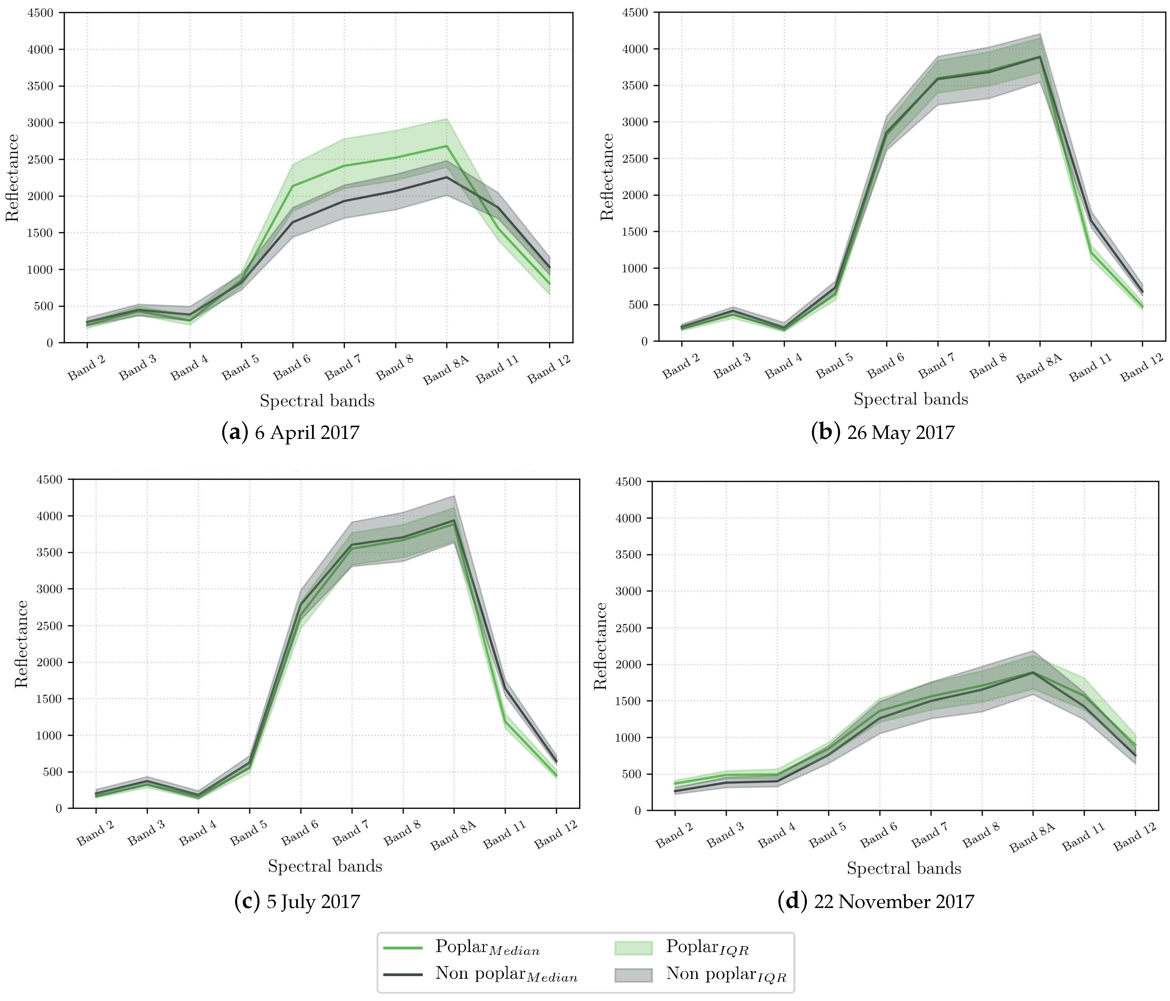
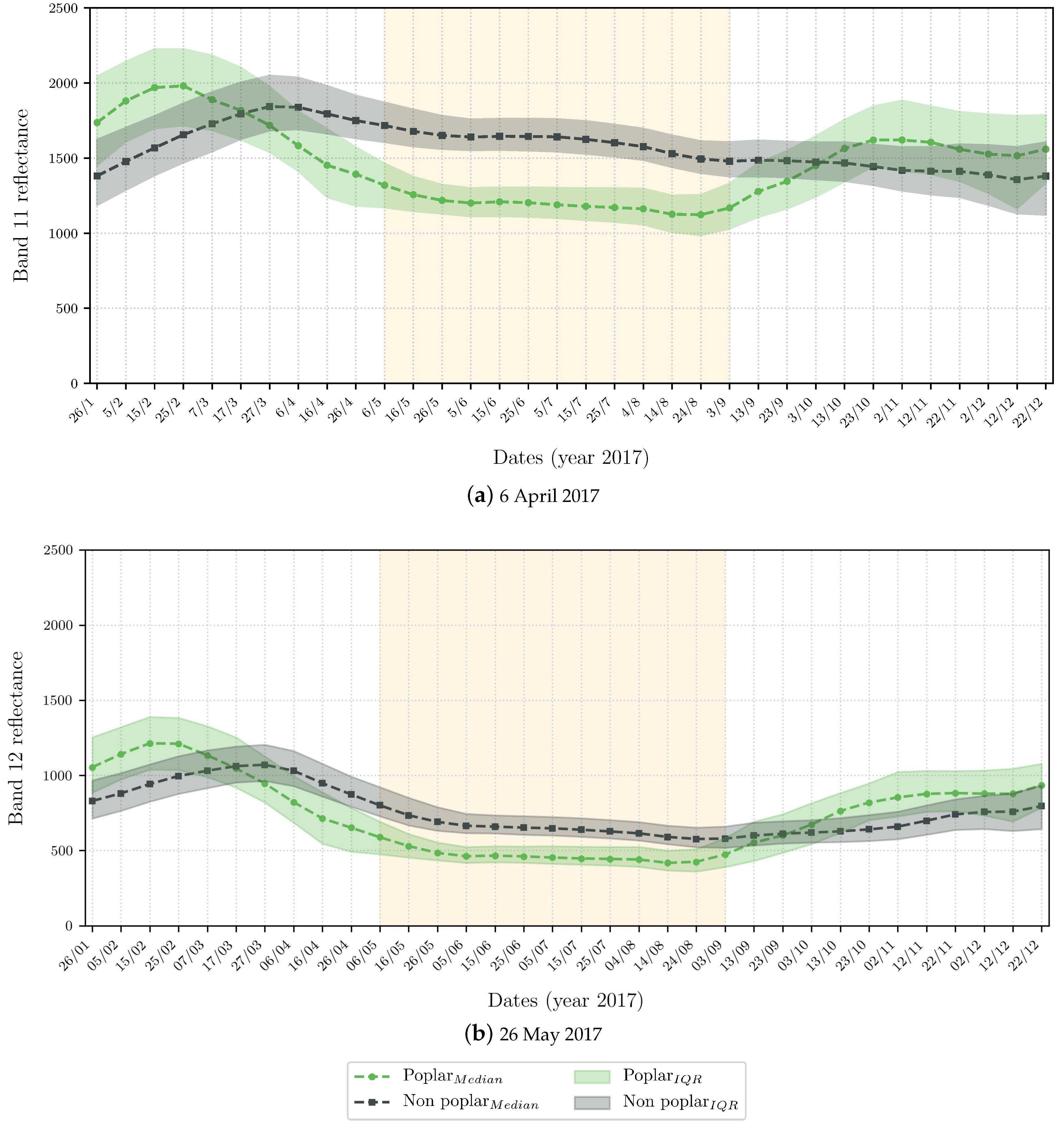
Prior to statistical processing, the spectral profiles were analysed visually and changes in poplar profiles over time evaluated by comparing the poplar reference samples and the other deciduous species (Figure 3). Beyond the expected phenological profile of deciduous trees and poplars (leaf emergence in spring and leaf senescence in autumn all over France), this analysis revealed a specific spectral pattern for poplars: from mid-April to early September, an absorption valley appeared in the SWIR bands B11 and B12, with no overlap with the other deciduous tree species (Figure 4). The reflectance of the SWIR bands decreased for all species during this period, but the decline was more pronounced for poplar plantations, especially in B11. This pattern was observed in both the 2017 and 2018 S2 time series.
Based on these observations, we established a new S2 poplar detection index (PI) with four variants (1, 2, 3, 4) as alternatives to spectral bands or existing spectral indices. The formulations are as follows:
PI 1 = B 11 B 12
PI 2 = B 5 ( B 11 + B 12 )
PI 3 = B 5 ( B 11 + B 12 ) B 5 + ( B 11 + B 12 )
PI 4 = B 11 + B 12
The PI 1 index is expressed as the difference between SWIR 1 (1610 nm) and SWIR 2 (2190 nm). This difference was more pronounced for poplar stands than for the other tree species. This was also true between SWIR 1 and other spectral bands (e.g., B8A, B8), but this difference was tested using other existing spectral indices (see below). The PI 2 index is defined as the addition of the two SWIR bands, which is then substracted to the red edge band (B5 centered at ∼704 nm). The interest of this formulation is using two wavelength regions and a spectral band with very close reflectance values for poplar stands and other species, in addition to the SWIR bands B11 and B12. This formulation accentuates the gaps. A normalised version is proposed with the PI 3 index. Other red edge bands (B6 and B7) were tested in the formulation of PI 2 and PI 3 , but we kept the best one (B5). The most intuitive PI 4 is a simple addition of the SWIR bands, which are expected to be lower for poplar stands. However, because PI 4 and PI 2 were highly correlated (Spearman’s ρ = 0.95 in 2017 and 0.93 in 2018; Appendix B), we excluded PI 4 from the multi-feature SFFS analysis. Results are only provided for the single-feature SFFS configuration. PI 2 was preferred because of the potential interest of the red edge band.
These new indices were compared to existing spectral indices. Here, we only selected standard indices (e.g., NDVI) or indices including SWIR bands or red edge domains (Table 3). A more exhaustive list of indices was tested, but for the sake of clarity, these less competitive indices are only reported in Appendix C.
A total of 16 spectral indices were computed for each S2 acquisition, resulting in 544 features in 2017 (i.e., 16 spectral indices × 34 dates) and 576 features in 2018 (36 dates). Using only spectral bands, the number of features was lower (340 and 360 for 2017 and 2018, respectively). In the single-feature SFFS configurations, the number of features for one band or one spectral index was directly linked to the number of acquisition dates (multi-temporal selection of a unique type of feature).

3.4. National Mapping of Poplar Plantations

The best subset of features identified by SFFS was retained to map poplar plantations at the national scale from a full model. For this purpose, we used the iota 2 processing chain, which is designed for operational land cover mapping at the country scale and enables optimal management of large volumes of satellite data [63].
Iota 2 was configured to use S2 data of the 2018 time series. All the images were subjected to the same pre-processing steps, including gap-filling, resampling of all bands to a 10 m spatial resolution, and temporal resampling with a 10-day step. The RF classification model was trained with the whole set of available references in the three study tiles and was then used to predict the 90 S2 tiles that cover the whole of France. The French Space Agency (CNES) computing infrastructure was used to process and store all the data.
Predictions in the resulting national map were partially masked with the freely available pan-European Copernicus High-Resolution Layers (HRL) 2018 forest layer of dominant leaf type at 10 m resolution (see https://land.copernicus.eu/pan-european/high-resolution-layers/forests (accessed on 4 January 2021)) to only retain pixels of forest with their membership class. The surface area of each poplar plantation in each municipality was then computed and mapped with its median confidence value.

4. Results

4.1. Multi-Feature SFFS

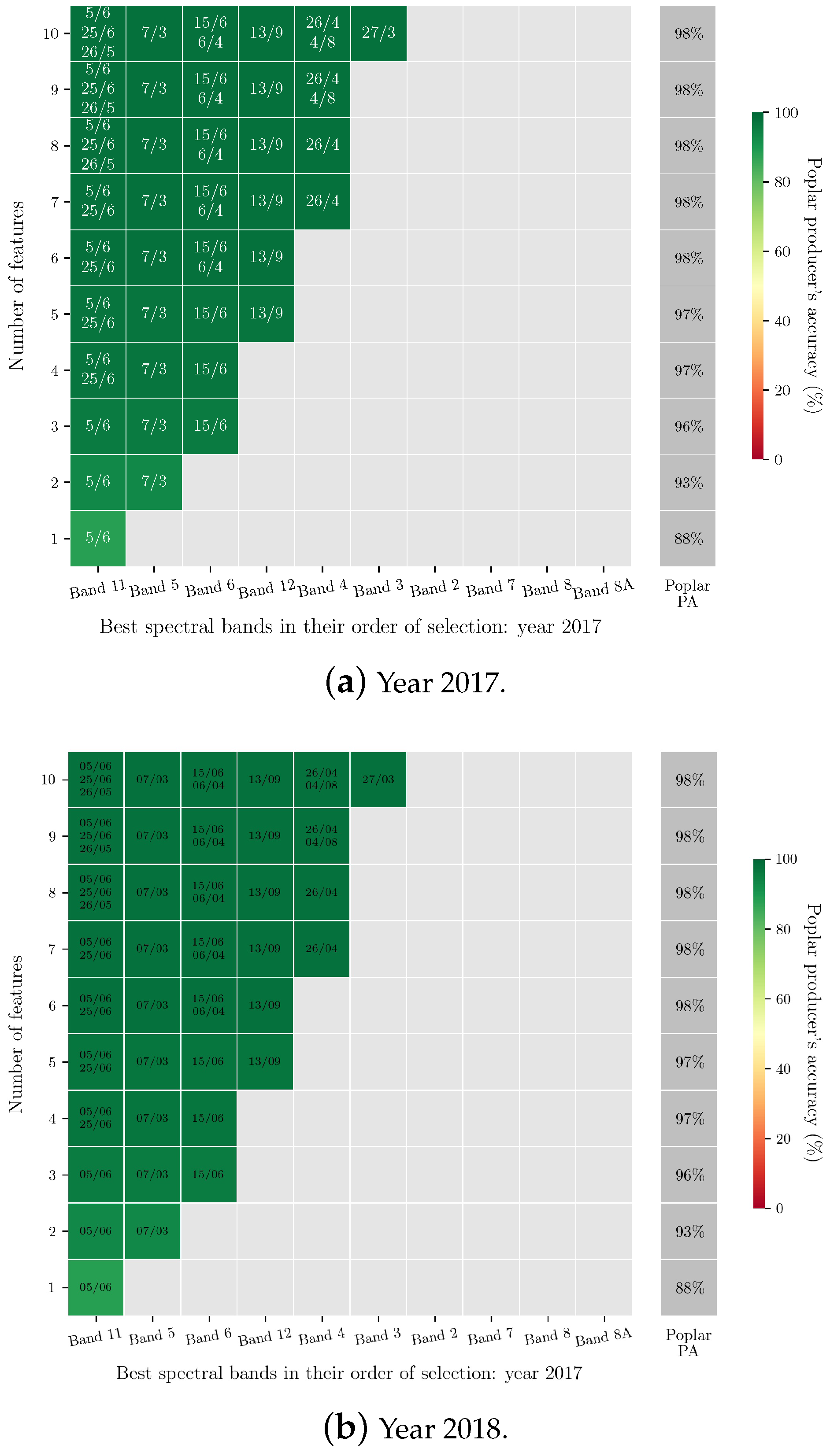
The results of feature selection with SFFS on the pool of spectral bands (i.e., multi-band configuration) are summarised in Figure 5. These graphs provide, for each number of features selected, the best performance achieved in terms of average poplar producer’s accuracy (PA, based on 5-fold CV), and the best bands selected with their corresponding dates.
In both years, the best band selected with SFFS was B11 (SWIR spectral range), which reached poplar PA values of 88% in 2017 and 90% in 2018 using one date. The dates of this best single feature were the 5th of June in 2017 and the 15th of July in 2018. In 2017 and 2018, the performance improved to, respectively, 98% and 99%, and then levelled off with the addition of six and five features belonging exclusively to the SWIR (B11 and B12) and red edge (B5 and B6) domains. Although the dates of the best feature subsets differed between the two years, the selection period was mainly from early spring (March) to late summer (September). In addition, despite the fact that SFFS can exclude some selected features in the newly updated set due to the floating search approach, we observed that each time a feature was selected, it was no longer excluded from the subset.
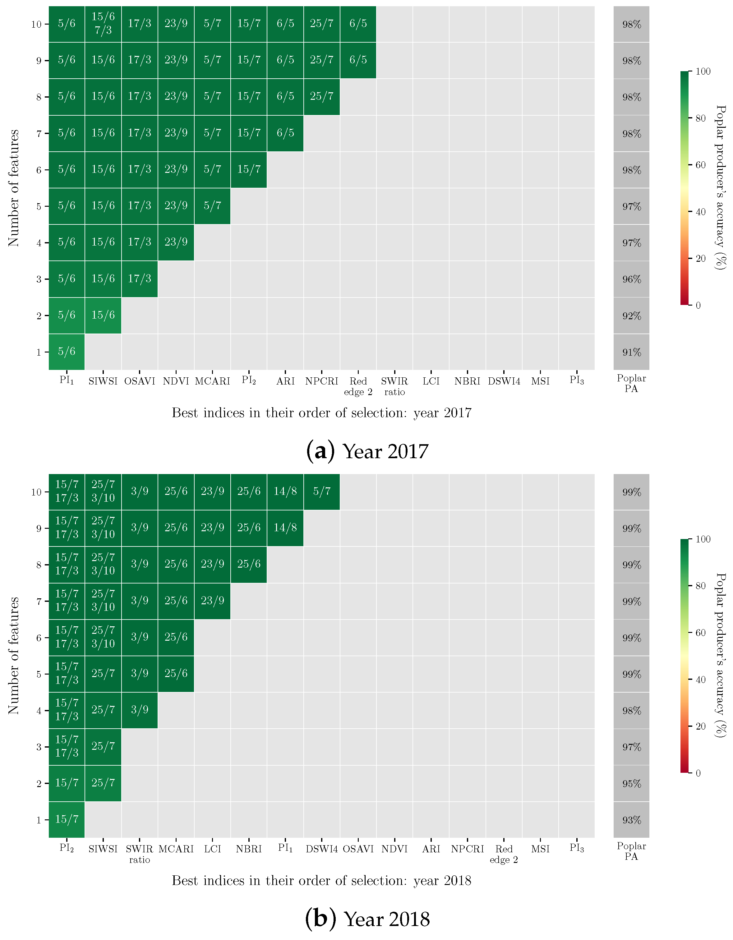
When feature selection was based on the spectral indices (i.e., multi-index configuration), the best first features differed between the two years (Figure 6). PI 1 emerged for 2017 (Figure 6a), while PI 2 was first selected for 2018 (Figure 6b). Considering only these indices, the poplar PA reached 91% in 2017 and 93% in 2018, that is, a difference of 3 percentage points to B11, which ranked first in the previous configuration. The dates of these first indices coincide with those of the best bands. The addition of other indices of different dates enabled maximum performance to be reached. Although the combination of indices differed in 2017 and 2018, some were the same (MCARI, SIWSI) in addition to PI 1 and PI 2 .
In these two multi-feature configurations involving all spectral bands or all spectral indices, the results highlight the interest of the SWIR and red edge domains, either by using the raw bands directly or by combining them in spectral indices. With a single feature, the multi-index configuration performed slightly better than the multi-band configuration. However, with the addition of new features, the two configurations performed equally well.
In both cases, and in the two years, although the best dates varied, the selected time period was from early spring (March) to late summer (September). In all cases, the best selected single feature matched a summer date (June or July). After the initial selection, no further features were removed from the subset.

4.2. Single-Feature SFFS

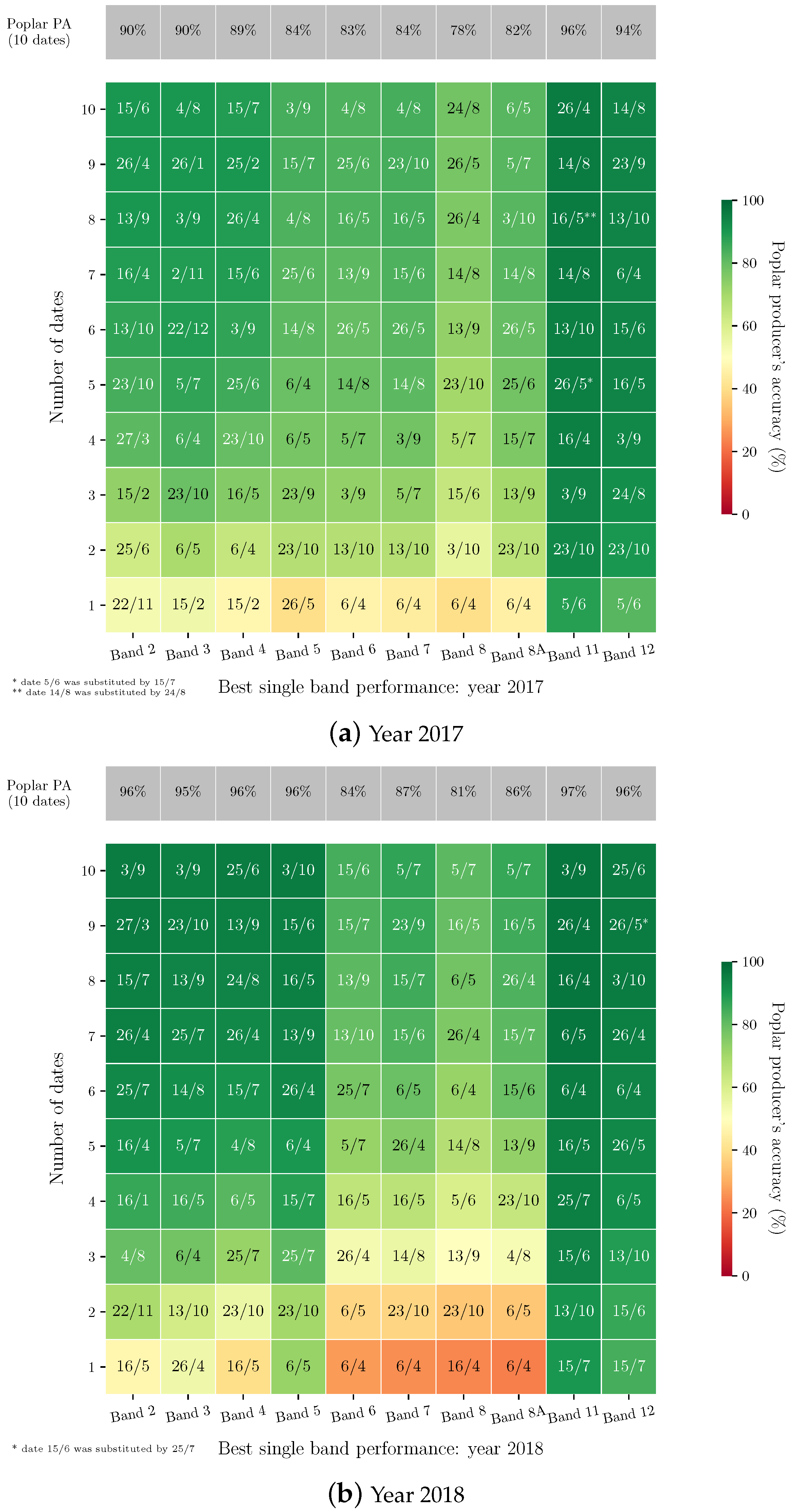
When we considered each spectral band separately and applied SFFS to all the dates in the 2017 (34 dates) and the 2018 (36 dates) time series, B11 and B12 from the SWIR spectral range achieved the best poplar PA values with the fewest features (Figure 7). Indeed, maximum performance was obtained with four features and reached 96% and 97% with B11 and 94% and 96% with B12 in 2017 and 2018, respectively. The performance was slightly better with B11 but was 2 percentage points lower than that achieved with the best combination of bands (i.e., in the multi-band configuration; Section 4.1).
Beyond four features, the PA values no longer increased. Some dates were eliminated immediately after being selected and sometimes re-integrated in the following subsets. This was the case with B11, for which the date of 14 August was introduced in the subset of seven features and replaced by the date of 24 August in the following subset of eight features but selected again in the subset of nine features.
B5 and B6 of the red edge ranked second in importance in the multi-band configuration after the SWIR bands, performed less well with the first dates, but improved to reach their maximum value after six features. For instance, the poplar’s PA of B5 was 40% with one date in 2017 but increased with additional dates and levelled off at 84%.
The same trend was observed for the remaining bands of the NIR (B7, B8, and B8A) and visible (B2, B3, and B4) domains whose initially low PA values increased with the addition of dates to reach their maximum performance, generally below that of the SWIR and red edge bands.
In the same SFFS configuration but using the 15 spectral indices, two stood out in both 2017 and 2018: PI 2 and SIWSI (Figure 8). The best poplar PA values were achieved from three features, scoring 96% and 98% with PI 2 and 96% and 97% with SIWSI in the two respective years. Other indices also produced similar performances in the two years, including PI 1 and MSI. Although PI 1 performed best in 2017 with only one date (poplar PA = 91%), PI 2 slightly outperformed it with three dates to achieve the highest poplar PA in this single-index configuration. In 2018, PI 2 always performed the best regardless of the number of dates.
Like in the multi-feature configuration, the selection period ranged mainly between spring and late summer/early autumn, with a shift in April instead of March (except for PI 4 ) and a shift in October instead of September. For the best features, the same summer dates were always identified first, namely the 5th of June in 2017 and the 15th of July in 2018.

4.3. Predictive Performances Using Another Independent Dataset

In the previous results, the predictive performance used to select features was based on a 5-fold CV applied on 50% of the reference dataset (i.e., the training set; see Section 3.2). Thus, the performances were computed on five independent subsets (named validation sets) by cross-validation. Here, performance values are given using the remaining 50% of references (i.e. the test set). The best results are summarised in Table 4 for each SFFS configuration and for both 2017 and 2018. The test score represents the poplar PA using the test set. The validation score represents the poplar PA based on cross-validation for comparison (results of Section 4.1 and Section 4.2). The results of both test and validation scores are based on the ten best subsets of features identified using SFFS.
We observed consistent results with the test set compared to validation scores. The performance gap between test and validation scores ranged from 3 to 27 percentage points depending on the year and the SFFS configuration. Using PI 2 in the single-feature configuration, the difference was 3 percentage points in 2017 and 4 percentage points in 2018, whereas using B5, it reached 27 and 16 percentage points, respectively, in 2017 and 2018.
Considering only the test set, the best performance in 2017 was obtained with PI 2 in the single-feature SFFS configuration with a poplar PA of 92%. In the multi-feature configuration, the combination of indices obtained the best PA (94%). According to the McNemar statistical test, the predictive performances differed significantly (p-values < 0.001; see Appendix D) in the single- and multi-index configurations, indicating that the combination of indices produced the best result in 2017. However, the combination of indices or bands (multi-feature configurations) produced equivalent performances (p-value = 0.395).
For the year 2018, PI 2 still produced the best performance of the single-feature configurations (see also confusion matrix in Appendix E for additional information on accuracy). The combination of bands ensured the highest poplar PA in the multi-feature configuration. In both cases, the poplar PA was 95%, with no significant difference (p-value = 0.523). The results of the other single- or multi-index configurations were less good.

4.4. National Map of Poplar Plantations Using the PI 2 Index

The first map of poplar plantations at the French national scale was produced for the year 2018 using the PI 2 index in a single-feature configuration. This simple configuration ensures optimal performance with stable results regardless of the year. A confidence map associated with the classification was also produced with a confidence level ranging from 0 to 100% for the class assigned to each pixel. The closer the confidence value to 100, the more confidence one can have in the algorithm for the predicted class.
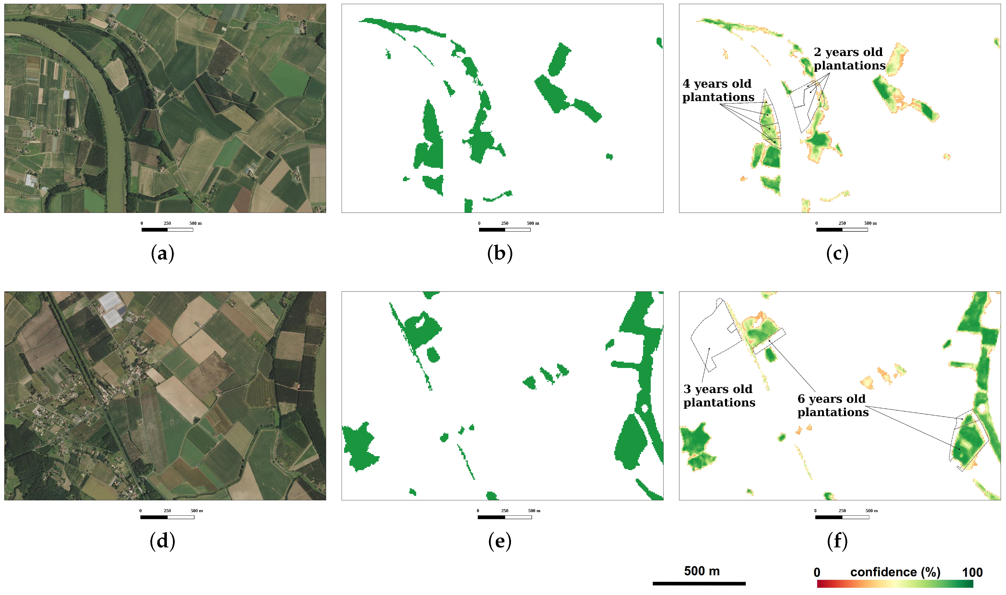
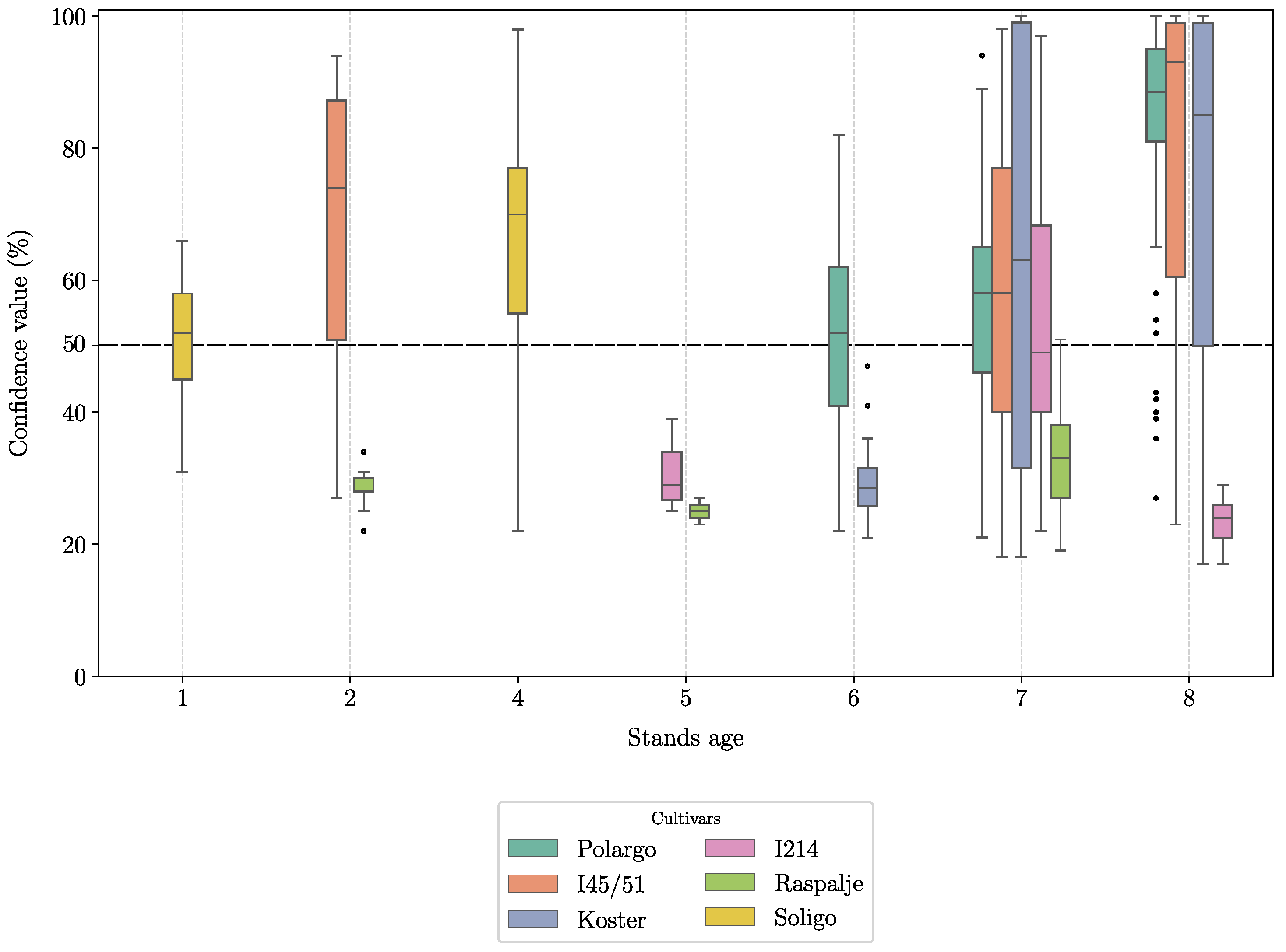
Some extracts are illustrated in Figure 9, Figure 10 and Figure 11. Mature plantations were generally well detected, with a high confidence level >= 75% (Figure 9). In contrast, young stands with limited canopy covers were either not mapped or detected with a confidence level of less than 50%. In some stands for which the year of plantation was known, as expected, plantations less than three years old were not detected. However, in the case of plantations between four and six years old, the age limit for detection varied. Indeed, in Figure 9c, four-year-old plantations were detected with a confidence level of between 50% and 90%, whereas in Figure 9f, six-year-old plantations were not systematically detected. This high variability of detection for young plantations has been analysed using the additional set of 85 field-checked polygons (see Section 2.2), highlighting the impact of the cultivar (Figure 12).
False positives in agricultural fields were also observed before masking non-forest areas (Figure 10a). In general, these cases were associated with low confidence values (<=25%) (Figure 10b) and can be excluded using a forest/non-forest mask (Figure 10c). Nevertheless, because of possible imperfections in the forest/non-forest mask, some poplar plantations with high confidence values were also excluded (see Figure 10f and Figure 11c).
Figure 13 shows the national map of poplar plantations with their prediction confidence level. A first estimate of the area under poplar based on pixel counting was produced for each municipality with either a low density of poplar trees with a high level of confidence (in blue) or the opposite, a high density of poplar trees with a low level of confidence (in yellow). Poplar forested areas are mainly distributed in north, central, and southwest France, as expected. Non-forest areas were masked using the 10 m Copernicus HRL 2018 forest layer. This mask helped to reduce over-detection in agricultural fields while retaining identified poplar stands.

5. Discussion

In this study, two years of 10-day resampled S2 time series were used to identify the optimal set of features and period needed to distinguish poplar plantations at broad scale. Based on a single-feature configuration using SFFS, we investigated the ability of specific wavelength regions and spectral indices with their respective dates to classify poplars. We also assessed the interest of combining multiple bands or indices using a multi-feature SFFS configuration. A new poplar detection index based on a SWIR and red edge S2 bands was defined and used to map plantations at the French countrywide scale. To our knowledge, this is the first attempt to analyse the most discriminating spectral regions of hybrid poplar plantations with S2 time series and to provide a S2-based poplar index to map poplar plantations including a large number of cultivars in different management contexts and over large areas.

5.1. Single-Feature vs. Multi-Feature: Less Is More

We observed no difference in accuracy between combinations of spectral bands or indices in the multi-feature configuration. This was true for both years even when only two features were selected. The results we obtained using single- and multi-feature configurations with the ten best feature subsets—whether by cross-validation or on another test set—were very close ( Δ P A 2 % ). The single PI 2 index at 10 dates provides almost the same performances as a combination of 8 different spectral bands at 8–10 dates or a combination of 8–9 spectral indices at 9 dates. This suggests that a simple approach based on a specific multi-temporal single feature is adapted to classify poplar plantations accurately. The temporal information compensates for the spectral information provided by the combination of multiple bands or indices. The increase in precision with an increase in the number of features obtained with the PI 2 index quickly reached a plateau beyond four features (i.e., dates) spread out between May and October. Thus, a very parsimonious approach with only few dates can be used to distinguish poplar plantations with the highest performance. This makes processing highly efficient in terms of computational complexity and load. This strategy for mapping poplars over large areas complements the previously defined strategy based on active learning [64]. The advantage of the latter is that it requires fewer reference samples, but its implementation involves a more complex learning process.

5.2. S2 Spectral Bands in the SWIR and Red Edge Domains Are Required to Identify Poplar

The results of variable selection with SFFS showed the relevance of the SWIR spectral region (B11 and B12) in distinguishing poplar plantations from other deciduous species. The results also highlighted the secondary importance of the red edge domain and particularly B5. Interestingly, these findings are in line with those reported by Viinikka et al. [23], who used airborne hyperspectral data with 460 spectral bands covering the visible, NIR, and SWIR ranges to discriminate European aspen from three other species in southern Finland. These authors found that the most discriminative bands of aspen trees were located in the red edge ( ρ 724 727 nm ) and SWIR ( ρ 1520 1564 nm and ρ 1684 1706 nm ) ranges. This does not perfectly fit the approximate wavelength range of B5 ( ρ 697 711 nm ) and B11 ( ρ 1565 1659 nm ) in Sentinel-2, but does refer to adjacent wavelengths.
Theoretically, the reflectance in the SWIR range is predominantly affected by leaf water content [65]. Changes in water content can be observed with the SWIR bands located near the major water absorption features at approximately the 1200 nm, 1450 nm, 1950 nm, and 2500 nm wavelengths of the spectrum [66], and most notably around 1450 nm and 1950 nm [67]. In case of high water contents, these absorptions bands become saturated, which induces a sensitivity to difference in leaf water content in the regions of intermediate absorptions near 1650 nm and 2200 nm [68], which coincides with B11 and B12 in S2. A high correlation between water status of Populus spp. and spectral indices based on SWIR bands (especially between 1500 and 1750 nm) was already observed in [69].
A number of remote sensing studies showed that SWIR bands’ reflectance decreased with an increase in leaf water content [65,70], suggesting that poplar leaves should have higher water content during the spring–summer period according to the results. This is consistent with the fact that high growth rate of poplar is associated with a high water demand. Irrigation, in addition to nutrient supply, is a common cultivation practice for poplar plantations [71]. For poplar, Zhang et al. [72] analysed seasonal (June to September) trends in the water consumption of trees in a temperate climate and showed that the increase in solar radiation was followed by an increase in evaporative demand. At the beginning of the summer season, the increase in transpiration was offset by an increase in the absorption of water available in the soil due to the typical capacity of poplar to exploit groundwater. Later in the season, soil water content decreased, and absorption reached a low plateau, leading to different adaptation mechanisms, such as stomatal closure to control losses through transpiration. This behaviour is consistent with the temporal profiles of the two SWIR bands, where in early spring (March), SWIR reflectance decreases rapidly as a result of increased water consumption to reach a low plateau, which continues throughout the dry season (July–August) (see Figure 4). Available information from past studies makes it hard to properly compare the seasonal variation of water contents between hybrid cultivated poplars and other deciduous trees with the corresponding spectral curves (e.g., see [73]). However, the LOPEX and ANGERS leaf optical properties databases provide water content values for different tree species [74,75]. For LOPEX, leaves were collected during early summer (June), and for some of them, also in early autumn (September). No information is provided for ANGERS. The poplar species available show rather high equivalent water thickness (EWT) values compared to other common tree species, especially Carolina poplar, which is a hybrid of P. x euramericana (Populus nigra x Populus deltoides), as we have in this study (Table 5). These values are independent of any irrigation practice.
However, the reflectance of vegetation canopies does not only depend on the leaf optical properties. Other factors are involved, such as viewing geometry and background signal, in addition to the canopy leaf area index (LAI) and the leaf angle distribution (LAD). Thus, at the stand level, the contribution of water content in spectral reflectance is modulated by these other factors [76,77]. Since high correlation may exist between SWIR bands and LAI (e.g., at 1650, 2100, and 2260 nm according to [78]), the variation in B11 and B12 may be related to the variation in LAI, in addition to water content. This is also true for spectral indices that exploit water absorption bands such as SIWSI, NBRI, and MSI [77]. The last one, whose performance was quite high in the single-index configuration, is correlated to the canopy LAI of poplar plantations [76]. More generally, in addition to the sensitivity towards water content, these indices respond to LAI and LAD in Sentinel-2 and possible other confounding structural drivers (e.g., stem density and crown diameter), as demonstrated by Morcillo-Pallarés et al. [77] from simulations at the leaf and forest canopy levels. Therefore, a possible functional convergence among optical traits could be suspected to explain the specific reflectance pattern of poplars in the SWIR bands.
An alternative assumption is the difference in phenolic compounds. More than 160 different types of phytochemical compounds have been identified in poplar species, including various phenolics including flavonoids, glucosides, acids, alcohol, lignan, and others [79]. Absorption features (depth, width, and area) centred near 1660 nm have been identified as robust indicators to quantify plant phenolic concentrations using reflectance spectra [80]. Variability in phenolics concentrations and compounds between poplar and non-poplar species may contribute to making B11 important. Further research is needed to verify this.
Concerning the red edge, this spectral region (680–780 nm) proved to be highly sensitive to the chlorophyll content of the vegetation [81,82] and has been used to estimate structural features such as LAI [83,84], or nutritional status such as N concentration (e.g., [85]). Recently, Kyaw et al. [86] showed that leaf reflectance of hybrid poplars at 712 nm (i.e., included in the B5 range) was a significant wavelength for predicting nitrogen content per unit leaf area (N a r e a ), even if the observed correlation was weak (R2 = 0.29 with a LASSO model). This relation was found using 105 leaf sample data of 62 Populus genotypes across seven taxa. Leaves were measured in July and early September in two young plantations located in upland regions of Mississippi, USA. In deciduous tree species, photosynthetic activity increases during the spring growing season (starting in March–April in temperate regions) along with the concentration of chlorophyll resulting from foliage growth [87,88]. Like with the SWIR bands, reflectance decreases at the start of the growing season, reflecting an increase in photosynthetic activity and in chlorophyll concentration [81]. The temporal signature of B5 reflects this trend with a decrease in reflectance from the end of March to mid-September (see Appendix F). However, only a marginal difference can be observed between plantations of poplar and those of other deciduous species, which may explain the minor importance of the red edge compared to that of SWIR for the discrimination of poplar plantations. The seasonal pattern of B5 suggests a possible higher chlorophyll content in poplars, especially in May and June, but this contradicts the low values available in the LOPEX and ANGERS leaf optical properties databases (Table 5). However, as for EWT, this comparison is rather unreliable because of the influence of the species-specific canopy structure on the spectral behaviour [89]. Further analysis is required to advance our understanding of the underlying biophysical process. It can be mentioned that S2 red edge band B5 was previously shown to be important for discriminating tree species in temperate forests, as well as SWIR bands B11 and B12 [90,91,92].
Finally, the PI 2 index, combining both B11 and B12 and subtracting them from B5, makes it possible to accentuate the difference between the reflectance of poplar and of other tree species. The lower the reflectances in the SWIR, the higher the value of PI 2 (Appendix F). This formulation was more competitive than the other variants of the Poplar index (PI 1 , PI 3 , PI 4 ) even if the results of PI 1 (based on B11 and B12 only) were very close to the results obtained in the single-index configuration. This was also true using B11 or B12 alone or the SIWSI spectral index (a normalised difference combining B11 and B8a), for which the difference in performance was significantly smaller (Appendix D). The PI index defined from S2 imagery could be adapted for other sensors, and in particular, Landsat 8-9 by selecting bands 6 (SWIR 1 at ∼1560–1660 nm) and 7 (SWIR 2 at ∼2100–2300 nm).

5.3. Poplar Recognition Is Not Driven by Phenological Differences with the Other Deciduous Species

Even if multitemporal data is required, our results show that the ability to discriminate poplar plantations from the other deciduous species is not related to subtle phenological differences in key periods of the vegetation cycle (e.g., timing of bud burst or leaf emergence). Recognition is possible because of a marked difference in spectral response, mainly in the SWIR bands (B11 and B12), throughout the growing season. The best dates selected using the Poplar index PI 2 are: 5 June, 25 July, 24 August, and 23 October in 2017 and 6 May, 25 June, 15 July, and 13 October in 2018. The first three dates are in the spring–summer period. The timing of flowering is already over, and the leaves are well developed. There is no specific phenological event during this period. By contrast, October coincides with the period of leaf senescence, with a yellowing phase. An important difference between poplar and the other deciduous species could explain the selection of this month. However, the senescence period of poplar overlaps with that of some other tree species, as observed in the spectral profiles. The temporal profiles of PI 2 for poplar and non-poplar classes show very close reflectance in October (as in late Winter, before March), suggesting an insignificant contribution of autumnal variations in species discrimination. Phenological differences are also reduced by the climate gradient due to the spatial extent (S2 image tiles were selected in contrasting climate regions) and by the existence of poplar cultivars with contrasting phenology (i.e., from early to late leaf emergence). At present, we have no clear explanation to understand the importance of the dates selected in October.

5.4. The National Map of Poplar Plantations Requires Field Validation

A first version of the national map was produced using the PI 2 index. As the feature selection analysis revealed, the map could have been produced using only a few dates between May and August, in addition to October, using this new index. However, because of cloudy acquisitions that vary from one region to another, the possible influence of residual noisy pixels (undetected clouds), and the existence of some evergreen deciduous species (e.g., eucalyptus plantations), we used the full year time series of PI 2 to generate the national map in 2018 (36 dates). After checking, we found that classification performances were not affected by the addition of all the dates (no Hughes phenomenon).
This map now needs to be validated in the field by forest partners to detect specific confusion with other species (missing from the reference set), the possible influence of the understorey vegetation in some regions where plantations were abandoned, and the detection limit related to the stage of development of the plantations. We assumed that no plantations less than three years old were mapped due to insufficient canopy cover and a possible effect of soil, but in practice, the minimum age for detection is more gradual because other factors have to be taken into consideration such as site conditions and the cultivar planted. Plantations can present different growth patterns with, for instance, a maximum growth rate in the first two years or a slow growth rate at the beginning and an increase in the growth rate later in the cycle [93,94]. We conducted a first analysis with a specific dataset of reference samples for which the cultivars and the age of the plantations were known. We observed an increase in the confidence values of the detected plantations with age, but this depended to a great extent on the cultivar concerned. Additional field-checked references are required to better define the detectability threshold of plantations. The absence of confusion with other short-rotation coppice (SRC) plantations, such as willow (Salix), which have higher water requirements, should also be verified. A previous study revealed a clear distinction between poplar and willow, but willow was growing in a natural context and not in SRC plantations [31].
The national map identified the main poplar plantation sites in France, but also a large number of municipalities with either a low density of poplar trees with a high level of confidence (in blue), or the opposite, a high density of poplar trees with a low level of confidence (in yellow). In the first case, in addition to the few plantations, this coincides with the presence of poplar in riparian areas. Some natural patches of poplar were detected along waterways. No precise evaluation was carried out to estimate the true ability to discriminate these poplars, but it opens up possibilities for such areas of high conservation value [95]. Over-detection was also observed in some places with low confidence values despite a high density of poplars. Closer examination revealed that these cases often refer to confusions with coniferous stands (or agricultural fields). From the modelling point of view, these errors are not surprising, since only references of deciduous species were used for training. Rather, they highlight the imperfection of the forest/non-forest mask used to only retain areas with deciduous species. The HRL Dominant Leaf Type 2018 was considered as the best candidate currently available, but its quality directly influenced our poplar plantation layer. In the future, the reference dataset could be enriched with conifer samples derived from the French NFI spatial database to distinguish between coniferous and deciduous trees in the classification process. An alternative would be the adoption of a novelty detection approach to identify test data (unseen pixels) that differ significantly from the training set [96]. This would make the method more independent of the existence of an accurate forest/non-forest mask.
We are confident about the accuracy of the French NFI spatial database and the way we used it as a reference dataset to limit classification bias. For the poplar class, the database was only used to identify a potential location of plantations, and each of them was checked by visual interpretation before integrating it into the reference dataset. Misidentification (evaluated by field campaigns) was considered negligible (<1%) and below the level that may affect the performance of the random forest classifier [97]. Moreover, unlike sub-natural forests, poplar plantations are monospecific and even-aged, composed of clones, which makes them very homogeneous and does not require a precise GPS survey to position trees. On the contrary, stands of other deciduous trees have not been checked. Therefore, it is possible that in some cases, the land use has changed or the species have been replaced by others since the year of the production of the forest database. According to the NFI statistics, the average timber extraction of deciduous trees from 2011 to 2019 is estimated at approximately 0.1 millions (M) m3/year in tile 31TCJ, 0.35 Mm3/year in tile 30TYT, and 0.55 Mm3/year in tile 31UEQ. The reference dataset can be affected by this noise. However, this imperfection should have a limited impact on poplar recognition because it mainly concerns the non-poplar class, with possible confusions between species within this class. Another source of imperfection is the possible existence of natural poplars in the mixed class of deciduous species. There is no specific pure class of natural poplars in the database, contrary to poplar plantations that are never assigned to the mixed class, whatever the stand area. In this case, the learning process could be affected, and some pixels of poplar could be predicted in the mixed class (and vice versa). Once again, this noise is probably too marginal to affect the model, and what appear to be confusions are not always in this case (see the matrix in Appendix E). Ultimately, we think that the most important bias for the countrywide prediction is the fact that the non-poplar class is not fully representative of the diversity of all the deciduous species. Only the species existing in the three image tiles were integrated. This limit can be easily overcome by collecting additional non-poplar references from the NFI spatial database in other image tiles.

6. Conclusions

The present study investigated the potential of S2 time series to discriminate poplar plantations over large areas, including their diversity related to cultivars, development stages, management practices, and climatic conditions.
Based on the results compared over two years, we draw the following conclusions:
  • There is no added value to be obtained by combining multiple spectral bands or different spectral indices at different dates to classify poplar accurately. If optimal features are selected, a multi-temporal single-feature approach provides equivalent results.
  • Only a few dates are required to identify poplar among deciduous species, the optimal period being the growing season; no significant improvement is achieved beyond four or five acquisition dates, but adding more dates can make the classification more robust to residual noise at the national scale without being affected by the curse of dimensionality (because of the single-feature strategy). Using the PI 2 poplar index, the best three dates are between May and August, with an additional date in October.
  • SWIR followed by red edge spectral regions are the most useful to differentiate poplars from other deciduous species. This reflects the sensitivity of poplar trees to water content throughout their phenological cycle. The best S2 spectral bands are B11, B12, B5, and B6. The best performances with stable results regardless of the year were obtained when some of these bands were combined through the PI 2 poplar index. Significant but limited differences were found with the PI 1 or SIWSI indices (which are the other competitive ones).
  • Because the model was trained using reference samples of deciduous species only, the national map of poplar plantations strongly depends on the quality of the forest/non-forest layer used to mask the unfocused areas.
The short-term future outlook of this work is to produce a national map of poplar plantations for other years. Comparing the different years should enable better evaluation of the potential errors in the maps, and limit a possible year effect in some regions. Comparing multi-year production is also the first step towards monitoring poplar resources and detecting harvest. It should help overcome the challenges related to young plantations, which were not reliably detected due to their open canopy but would become detectable over the years.
Another future objective is to make the approach less dependent on the availability and quality of a forest/non-forest mask. The detection of forest tree cover before distinguishing poplar is one possible option, based on S2, but also multitemporal Sentinel-1 data [98]. This would ensure an up-to-date mask for each annual production of the poplar layer.

Author Contributions

Conceptualisation, Y.H. and D.S.; methodology, Y.H. and D.S.; software, Y.H.; validation, Y.H., D.S., V.C., C.M. and E.P.; formal analysis, Y.H.; investigation, Y.H.; data curation, Y.H.; writing—original draft preparation, Y.H. and D.S.; writing—review and editing, Y.H., D.S., V.C., C.M. and E.P.; visualisation, Y.H. and D.S.; supervision, D.S., V.C., C.M. and E.P.; project administration, D.S.; funding acquisition, D.S. and E.P. All authors have read and agreed to the published version of the manuscript.

Funding

This work was supported by public funding from the French Ministry of Food and Agriculture, the French Ministry of Higher Education and Research, the regions of Nouvelle Aquitaine and Grand Est, and the County Council of Lot-et-Garonne. The project also involved private funders, namely the Codifab, France Bois Forêt, Alliance Forêts Bois, and the company Garnica Plywood. The study has also received financial support from the French Space Agency CNES, as part of TOSCA Parcelle project.

Data Availability Statement

Not applicable.

Conflicts of Interest

The authors declare no conflict of interest.

Appendix A. Resampled Dates for 2017 and 2018 Time Series

Table A1. Common resampled dates over 2017 and 2018 time series.
Resampled Dates (in 2017)Resampled Dates (in 2018)
NA6 January 2018
NA16 January 2018
26 January 201726 January 2018
5 February 20175 February 2018
15 February 201715 February 2018
25 February 201725 February 2018
7 March 20177 March 2018
17 March 201717 March 2018
27 March 201727 March 2018
6 April 20176 April 2018
16 April 201716 April 2018
26 April 201726 April 2018
6 May 20176 May 2018
16 May 201716 May 2018
26 May 201726 May 2018
5 June /20175 June 2018
15 June 201715 June 2018
25 June /201725 June 2018
5 July 20175 July 2018
15 July 201715 July 2018
25 July 201725 July 2018
4 August 20174 August 2018
14 August 201714 August 2018
24 August 201724 August 2018
3 September 20173 September 2018
13 September 201713 September 2018
23 September /201723 September 2018
3 October 20173 October 2018
13 October 201713 October 2018
23 October 201723 October 2018
2 November 20172 November 2018
12 November 201712 November 2018
22 November 201722 November 2018
2 December /20172 December 2018
12 December 201712 December 2018
22 December 201722 December 2018

Appendix B. Correlation between the Poplar Index (PI) Variants
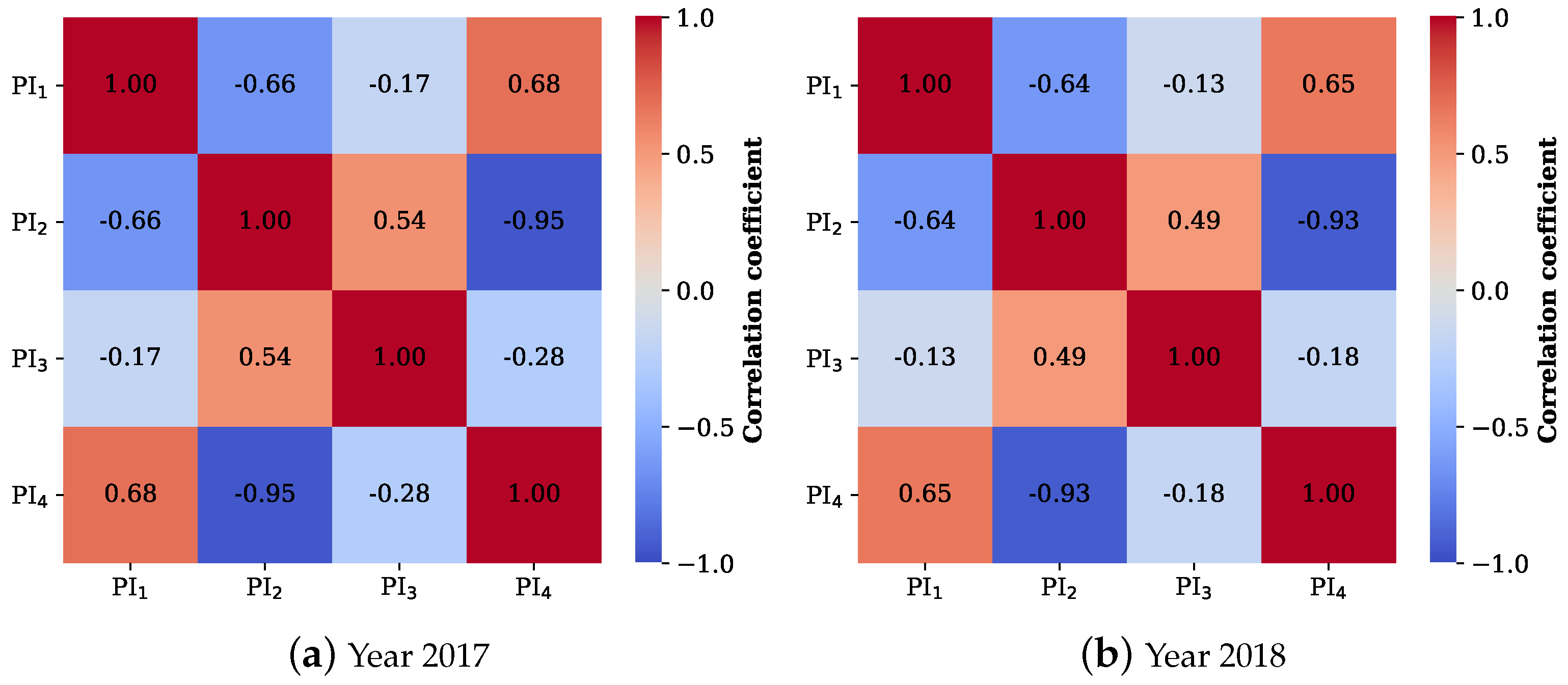
Figure A1. Spearman’s ρ correlation coefficients between poplar index (PI) variants based on all resampled dates for 2017 and 2018 S2 time series.
Remotesensing 14 03975 g0a1

Appendix C. Additional Spectral Indices Tested

Table A2. List of additional spectral indices tested and their corresponding formulas.
IndicesFormulasReferences
Normalised Difference Moisture IndexNDMI = B 8 B 11 B 8 + B 11 [99]
Normalised Difference Snow IndexNDSI = B 3 B 11 B 3 + B 11 [100]
Normalised Difference Water IndexNDWI = B 3 B 8 B 3 + B 8 [65]
Bare Soil IndexBSI = ( B 11 + B 4 ) ( B 8 + B 2 ) ( B 11 + B 4 ) + ( B 8 + B 2 ) [101]
Normalised Difference Salinity IndexNDSI2 = B 11 B 12 B 11 + B 12 [102]
Burned Area Index for Sentinel-2BAIS2 = ( 1 B 6 B 7 B 8 A B 4 ) ( B 12 B 8 A B 12 + B 8 A + 1 ) [103]
Inverted Red-Edge Chlorophyll IndexIRECI = B 7 B 4 B 5 B 6 [104]

Appendix D. McNemar Test p-Values

Table A3. Classification comparison with the p-values derived from the McNemar significance test of performance on the test set. Values less than the significance level of α = 0.05 indicate a statistically significant difference between the two models at the 95% confidence interval. Otherwise, if the p-values > α (highlighted in bold), the null hypothesis cannot be rejected.
Band 11Band 12PI 2 SIWSIBandsIndicesPI 1 PI 3 PI 4
Year
2017
Band 5<0.001<0.001<0.001<0.00100<0.001<0.001<0.001
Band 11-<0.001<0.001<0.001<0.001<0.001<0.001<0.001<0.001
Band 12--<0.0010.097<0.001<0.001<0.001<0.0010.041
PI 2 ---<0.001<0.001<0.001<0.001<0.001<0.001
SIWSI----<0.001<0.001<0.001<0.0010.014
Bands-----0.395<0.001<0.001<0.001
Indices------<0.001<0.001<0.001
PI 1 -------<0.001<0.001
PI 3 --------<0.001
Year
2018
Band 5<0.001<0.001<0.001<0.001<0.001<0.001<0.001<0.001<0.001
Band 11-<0.001<0.001<0.001<0.001<0.001<0.001<0.0010.015
Band 12--<0.001<0.001<0.001<0.0010.069<0.001<0.001
PI 2 ---<0.0010.523<0.001<0.0010<0.001
SIWSI----<0.001<0.001<0.001<0.001<0.001
Bands-----<0.001<0.0010<0.001
Indices------<0.0010<0.001
PI 1 -------<0.001<0.001
PI 3 --------<0.001
Table A4. Poplar PA scores achieved with the ten best feature subsets based on SFFS in the single-feature configuration using the three variants of the poplar index: PI 1 , PI 3 , and PI 4 . The test score gives the poplar PA after prediction on the test set (50% of reference data). These values are significantly lower than the best PA scores obtained with PI 2 : 92% in 2017 and 95% in 2018 (see Table 4 in the core of the manuscript).
YearPoplar PA ScoresPI 1 PI 3 PI 4
2017test score84.973.988.3
2018test score89.773.392.2

Appendix E. Confusion Matrix of the Classification Based on PI2 in the Single-Feature Configuration for Year 2018
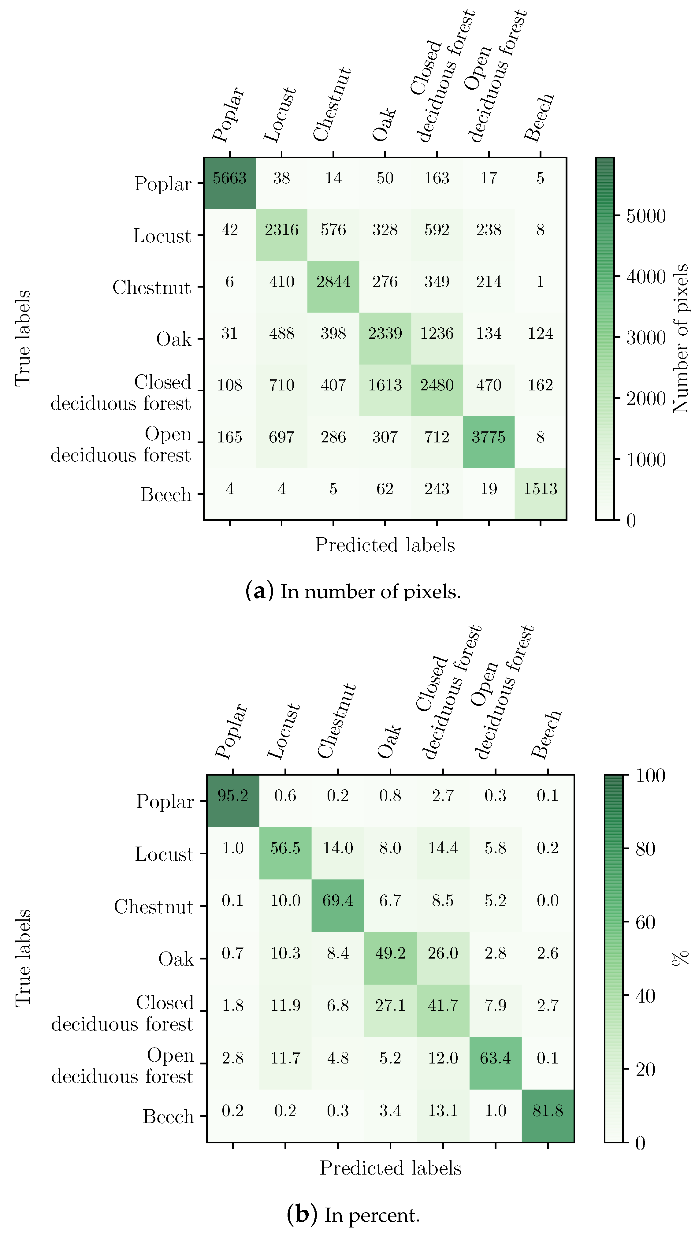
Figure A2. Confusion matrix in (a) pixels and (b) percent. The PA of poplar class is 95%. The UA is 94%, and the F-score is 94.5%.
Remotesensing 14 03975 g0a2

Appendix F. Spectral Signatures

Figure A3. Temporal profile of band 5 reflectance in poplar plantations versus other deciduous tree species: in (a), the profile in 2017; in (b), the profile in 2018. Dashed lines refer to the median signal, and the surrounding shaded areas represent the interquartile range, shown in red for poplar and in grey for other deciduous species. The light yellow box highlights the most discriminating spring–summer period for poplars.
Remotesensing 14 03975 g0a3
Figure A4. Temporal profile of band 12 reflectance in poplar plantations versus other deciduous tree species: in (a), the profile in 2017; in (b), the profile in 2018. Dashed lines refer to the median signal, and the surrounding shaded areas represent the interquartile range, shown in red for poplar and in grey for other deciduous species. The light yellow box highlights the most discriminating spring–summer period for poplars.
Remotesensing 14 03975 g0a4
Figure A5. Temporal profile of PI 2 reflectance in poplar plantations versus other deciduous tree species: in (a), the profile in 2017; in (b), the profile in 2018. Dashed lines refer to the median signal, and the surrounding shaded areas represent the interquartile range, shown in purple for poplar and in grey for other deciduous species. The light yellow box highlights the most discriminating spring–summer period for poplars.
Remotesensing 14 03975 g0a5

References

  1. Fares, S.; Mugnozza, G.; Corona, P.; Palahí, M. Sustainability: Five steps for managing Europe’s forests. Nature 2015, 519, 407–409. [Google Scholar] [CrossRef] [PubMed]
  2. FAO. Global Forest Resources Assessment 2020: Key Findings; FAO: Rome, Italy, 2020. [Google Scholar]
  3. Carle, J.; Holmgren, P. Wood from planted forests. For. Prod. J. 2008, 58, 6. [Google Scholar]
  4. FAO. Poplars and Other Fast-Growing Trees—Renewable Resources for Future Green Economies; Synthesis of Country Progress Reports: Berlin, Germany, 2016. [Google Scholar]
  5. Boyd, D.; Danson, F. Satellite remote sensing of forest resources: Three decades of research development. Prog. Phys. Geogr. 2005, 29, 1–26. [Google Scholar] [CrossRef]
  6. Reitberger, J.; Krzystek, P.; Stilla, U. Analysis of Full Waveform LIDAR Data for the Classification of Deciduous and Coniferous Trees. Int. J. Remote Sens. 2008, 29, 1407–1431. [Google Scholar] [CrossRef]
  7. Hansen, J.; Mitchard, E.A.; King, S. Assessing Forest/Non-Forest Separability Using Sentinel-1 C-Band Synthetic Aperture Radar. Remote Sens. 2020, 12, 1899. [Google Scholar] [CrossRef]
  8. Immitzer, M.; Atzberger, C.; Koukal, T. Tree Species Classification with Random Forest Using Very High Spatial Resolution 8-Band WorldView-2 Satellite Data. Remote Sens. 2012, 4, 2661–2693. [Google Scholar] [CrossRef]
  9. Sheeren, D.; Fauvel, M.; Josipović, V.; Lopes, M.; Planque, C.; Willm, J.; Dejoux, J.F. Tree Species Classification in Temperate Forests Using Formosat-2 Satellite Image Time Series. Remote Sens. 2016, 8, 734. [Google Scholar] [CrossRef]
  10. Fassnacht, F.E.; Latifi, H.; Stereńczak, K.; Modzelewska, A.; Lefsky, M.; Waser, L.T.; Straub, C.; Ghosh, A. Review of Studies on Tree Species Classification from Remotely Sensed Data. Remote Sens. Environ. 2016, 186, 64–87. [Google Scholar] [CrossRef]
  11. Persson, M.; Lindberg, E.; Reese, H. Tree Species Classification with Multi-Temporal Sentinel-2 Data. Remote Sens. 2018, 10, 1794. [Google Scholar] [CrossRef]
  12. Torbick, N.; Ledoux, L.; Salas, W.; Zhao, M. Regional Mapping of Plantation Extent Using Multisensor Imagery. Remote Sens. 2016, 8, 236. [Google Scholar] [CrossRef]
  13. Li, Z.; Fox, J.M. Mapping Rubber Tree Growth in Mainland Southeast Asia Using Time-Series MODIS 250 m NDVI and Statistical Data. Appl. Geogr. 2012, 32, 420–432. [Google Scholar] [CrossRef]
  14. Ye, S.; Rogan, J.; Sangermano, F. Monitoring Rubber Plantation Expansion Using Landsat Data Time Series and a Shapelet-Based Approach. ISPRS J. Photogramm. Remote Sens. 2018, 136, 134–143. [Google Scholar] [CrossRef]
  15. Xiao, C.; Li, P.; Feng, Z. Monitoring Annual Dynamics of Mature Rubber Plantations in Xishuangbanna during 1987-2018 Using Landsat Time Series Data: A Multiple Normalization Approach. Int. J. Appl. Earth Obs. Geoinf. 2019, 77, 30–41. [Google Scholar] [CrossRef]
  16. Puttinaovarat, S.; Horkaew, P. Deep and Machine Learnings of Remotely Sensed Imagery and Its Multi-Band Visual Features for Detecting Oil Palm Plantation. Earth Sci. Inform. 2019, 12, 429–446. [Google Scholar] [CrossRef]
  17. Descals, A.; Szantoi, Z.; Meijaard, E.; Sutikno, H.; Rindanata, G.; Wich, S. Oil Palm (Elaeis Guineensis) Mapping with Details: Smallholder versus Industrial Plantations and Their Extent in Riau, Sumatra. Remote Sens. 2019, 11, 2590. [Google Scholar] [CrossRef]
  18. Le Maire, G.; Dupuy, S.; Nouvellon, Y.; Loos, R.A.; Hakamada, R. Mapping Short-Rotation Plantations at Regional Scale Using MODIS Time Series: Case of Eucalypt Plantations in Brazil. Remote Sens. Environ. 2014, 152, 136–149. [Google Scholar] [CrossRef]
  19. Forstmaier, A.; Shekhar, A.; Chen, J. Mapping of Eucalyptus in Natura 2000 Areas Using Sentinel 2 Imagery and Artificial Neural Networks. Remote Sens. 2020, 12, 2176. [Google Scholar] [CrossRef]
  20. Deng, X.; Guo, S.; Sun, L.; Chen, J. Identification of Short-Rotation Eucalyptus Plantation at Large Scale Using Multi-Satellite Imageries and Cloud Computing Platform. Remote Sens. 2020, 12, 2153. [Google Scholar] [CrossRef]
  21. Spracklen, B.; Spracklen, D.V. Synergistic Use of Sentinel-1 and Sentinel-2 to Map Natural Forest and Acacia Plantation and Stand Ages in North-Central Vietnam. Remote Sens. 2021, 13, 185. [Google Scholar] [CrossRef]
  22. Heyman, O.; Gaston, G.; Kimerling, A.; Campbell, J. A Per-Segment Approach to Improving Aspen Mapping from High-Resolution Remote Sensing Imagery. J. For. 2003, 101, 29–33. [Google Scholar]
  23. Viinikka, A.; Hurskainen, P.; Keski-Saari, S.; Kivinen, S.; Tanhuanpää, T.; Mäyrä, J.; Poikolainen, L.; Vihervaara, P.; Kumpula, T. Detecting European Aspen (Populus Tremula L.) in Boreal Forests Using Airborne Hyperspectral and Airborne Laser Scanning Data. Remote Sens. 2020, 12, 2610. [Google Scholar] [CrossRef]
  24. Kivinen, S.; Koivisto, E.; Keski-Saari, S.; Poikolainen, L.; Tanhuanpää, T.; Kuzmin, A.; Viinikka, A.; Heikkinen, R.K.; Pykälä, J.; Virkkala, R.; et al. A Keystone Species, European Aspen (Populus Tremula L.), in Boreal Forests: Ecological Role, Knowledge Needs and Mapping Using Remote Sensing. For. Ecol. Manag. 2020, 462, 118008. [Google Scholar] [CrossRef]
  25. Chardenon, J.; Flouzat, G. The application of remote sensing to poplar growing: Identification and inventory of poplar groves, prediction of timber production; France, Italy. Rev. For. Fr. 1981, 33, 478–493. [Google Scholar] [CrossRef]
  26. Borry, F.C.; de Roover, B.P.; Leysen, M.M.; de Wulf, R.R.; Goossens, R.E. Evaluation of SPOT and TM Data for Forest Stratification: A Case Study for Small-Size Poplar Stands. IEEE Trans. Geosci. Remote Sens. 1993, 31, 483–490. [Google Scholar] [CrossRef]
  27. Grignetti, A.; Coaloa, D.; Niccolini, G. Classification of poplar stand areas by high-resolution satellite images. Forest 2009, 6, 299–311. [Google Scholar] [CrossRef]
  28. Eslami, A.; Zahedi, S.S. Providing Poplar Plantation Map by Indian Remote Sensing (IRS) Satellite Imagery in Northern Iran. Afr. J. Agric. Res. 2011, 6, 4769–4774. [Google Scholar]
  29. D’Amico, G.; Francini, S.; Giannetti, F.; Vangi, E.; Travaglini, D.; Chianucci, F.; Mattioli, W.; Grotti, M.; Puletti, N.; Corona, P.; et al. A deep learning approach for automatic mapping of poplar plantations using Sentinel-2 imagery. Gisci. Remote Sens. 2021, 58, 1352–1368. [Google Scholar] [CrossRef]
  30. Hościło, A.; Lewandowska, A. Mapping Forest Type and Tree Species on a Regional Scale Using Multi-Temporal Sentinel-2 Data. Remote Sens. 2019, 11, 929. [Google Scholar] [CrossRef]
  31. Karasiak, N.; Dejoux, J.F.; Fauvel, M.; Willm, J.; Monteil, C.; Sheeren, D. Statistical Stability and Spatial Instability in Mapping Forest Tree Species by Comparing 9 Years of Satellite Image Time Series. Remote Sens. 2019, 11, 2512. [Google Scholar] [CrossRef]
  32. Joly, D.; Brossard, T.; Cardot, H.; Cavailhes, J.; Hilal, M.; Wavresky, P. Les types de climats en France, une construction spatiale. Cybergeo Eur. J. Geogr. 2010, 501, 34–42. [Google Scholar] [CrossRef]
  33. IGN. La forêt plantée en France: état des lieux. L’If Feuille L’Inventaire For. 2017, 40, 10–11. [Google Scholar]
  34. Hagolle, O.; Huc, M.; Villa Pascual, D.; Dedieu, G. A Multi-Temporal and Multi-Spectral Method to Estimate Aerosol Optical Thickness over Land, for the Atmospheric Correction of FormoSat-2, LandSat, VENμS and Sentinel-2 Images. Remote Sens. 2015, 7, 2668–2691. [Google Scholar] [CrossRef]
  35. Inglada, J.; Vincent, A.; Arias, M.; Marais-Sicre, C. Improved Early Crop Type Identification By Joint Use of High Temporal Resolution SAR And Optical Image Time Series. Remote Sens. 2016, 8, 362. [Google Scholar] [CrossRef]
  36. Boureau, J.G. Manuel d’Interprétation des Photographies Aériennes Infrarouges; IFN: Saint-Jean-de-la-Ruelle, France, 2008. [Google Scholar]
  37. Jia, X.; Kuo, B.C.; Crawford, M.M. Feature Mining for Hyperspectral Image Classification. Proc. IEEE 2013, 101, 676–697. [Google Scholar] [CrossRef]
  38. Chandrashekar, G.; Sahin, F. A survey on feature selection methods. Comput. Electr. Eng. 2014, 40, 16–28. [Google Scholar] [CrossRef]
  39. Hughes, G. On the mean accuracy of statistical pattern recognizers. IEEE Trans. Inf. Theory 1968, 14, 55–63. [Google Scholar] [CrossRef]
  40. Pudil, P.; Novovičová, J.; Kittler, J. Floating Search Methods in Feature Selection. Pattern Recognit. Lett. 1994, 15, 1119–1125. [Google Scholar] [CrossRef]
  41. Gomez-Chova, L.; Calpe, J.; Camps-Valls, G.; Martin, J.; Soria, E.; Vila, J.; Alonso-Chorda, L.; Moreno, J. Feature selection of hyperspectral data through local correlation and SFFS for crop classification. In Proceedings of the IEEE International Geoscience and Remote Sensing Symposium (IGARSS), Toulouse, France, 21–25 July 2003; Volume 1, pp. 555–557. [Google Scholar]
  42. Le Bris, A.; Chehata, N.; Briottet, X.; Paparoditis, N. Use intermediate results of wrapper band selection methods: A first step toward the optimization of spectral configuration for land cover classifications. In Proceedings of the 6th Workshop on Hyperspectral Image and Signal Processing: Evolution in Remote Sensing (WHISPERS), Lausanne, Switzerland, 24–27 June 2014; pp. 1–4. [Google Scholar]
  43. Karasiak, N.; Dejoux, J.F.; Monteil, C.; Sheeren, D. Spatial dependence between training and test sets: Another pitfall of classification accuracy assessment in remote sensing. Mach. Learn. 2022, 111, 2715–2740. [Google Scholar] [CrossRef]
  44. Breiman, L. Random Forests. Mach. Learn. 2001, 45, 5–32. [Google Scholar] [CrossRef]
  45. Ghosh, A.; Joshi, P.K. A Comparison of Selected Classification Algorithms for Mapping Bamboo Patches in Lower Gangetic Plains Using Very High Resolution WorldView 2 Imagery. Int. J. Appl. Earth Obs. Geoinf. 2014, 26, 298–311. [Google Scholar] [CrossRef]
  46. Foody, G.M. Explaining the Unsuitability of the Kappa Coefficient in the Assessment and Comparison of the Accuracy of Thematic Maps Obtained by Image Classification. Remote Sens. Environ. 2020, 239, 111630. [Google Scholar] [CrossRef]
  47. McNemar, Q. Note on the Sampling Error of the Difference between Correlated Proportions or Percentages. Psychometrika 1947, 12, 153–157. [Google Scholar] [CrossRef] [PubMed]
  48. Dietterich, T.G. Approximate Statistical Tests for Comparing Supervised Classification Learning Algorithms. Neural Comput. 1998, 10, 1895–1923. [Google Scholar] [CrossRef]
  49. Foody, G.M. Thematic Map Comparison: Evaluating the Statistical Significance of Differences in Classification Accuracy. Photogramm. Eng. Remote Sens. 2004, 70, 627–633. [Google Scholar] [CrossRef]
  50. Raschka, S. MLxtend: Providing machine learning and data science utilities and extensions to Python’s scientific computing stack. J. Open Source Softw. 2018, 3, 638. [Google Scholar] [CrossRef]
  51. Pedregosa, F.; Varoquaux, G.; Gramfort, A.; Michel, V.; Thirion, B.; Grisel, O.; Blondel, M.; Prettenhofer, P.; Weiss, R.; Dubourg, V.; et al. Scikit-Learn: Machine Learning in Python. J. Mach. Learn. Res. 2011, 12, 2825–2830. [Google Scholar]
  52. Rouse, J.; Haas, R.H.; Schell, J.A.; Deering, D. Monitoring vegetation systems in the Great Plains with ERTS. In Proceedings of the 3rd Earth Resources Technology Satellite-1 Symposium, Washington, DC, USA, 10–14 December 1973; NASA Scientific and Technical Information Office: Washington, DC, USA, 1974; Volume 1, pp. 309–317. [Google Scholar]
  53. Hunt, E.; Rock, B.N. Detection of changes in leaf water content using Near- and Middle-Infrared reflectances. Remote Sens. Environ. 1989, 30, 43–54. [Google Scholar]
  54. Apan, A.; Held, A.; Phinn, S.; Markley, J. Formulation and Assessment of Narrow-Band Vegetation Indices from EO-1 Hyperion Imagery for Discriminating Sugarcane Disease. In Proceedings of the Spatial Sciences Institute Biennial Conference (SSC 2003), Canberra, Australia, 22–26 September 2003; Spatial Knowledge Without Boundaries. Spatial Sciences Institute: Canberra, Australia, 2003; pp. 1–13. [Google Scholar]
  55. Peñuelas, J.; Gamon, J.A.; Fredeen, A.L.; Merino, J.; Field, C.B. Reflectance Indices Associated with Physiological Changes in Nitrogen- and Water-Limited Sunflower Leaves. Remote Sens. Environ. 1994, 48, 135–146. [Google Scholar] [CrossRef]
  56. Key, C.; Benson, N. Landscape Assessment: Ground Measure of Severity, the Composite Burn Index; and Remote Sensing of Severity, the Normalized Burn Ratio. In FIREMON: Fire Effects Monitoring and Inventory System; USDA Forest Service: Washington, DC, USA, 2006; pp. LA1–51. [Google Scholar]
  57. Fensholt, R.; Sandholt, I. Derivation of a Shortwave Infrared Water Stress Index from MODIS Near- and Shortwave Infrared Data in a Semiarid Environment. Remote Sens. Environ. 2003, 87, 111–121. [Google Scholar] [CrossRef]
  58. Gitelson, A.A.; Merzlyak, M.; Zur, Y.; Stark, R.; Gritz, U. Non-destructive and remote sensing techniques for estimation of vegetation status. In Proceedings of the 3rd European Conference on Precision Agriculture, Montpellier, France, 18–20 June 2001; pp. 205–210. [Google Scholar]
  59. Rondeaux, G.; Steven, M.; Baret, F. Optimization of Soil-Adjusted Vegetation Indices. Remote Sens. Environ. 1996, 55, 95–107. [Google Scholar] [CrossRef]
  60. Datt, B. Remote Sensing of Water Content in Eucalyptus Leaves. Aust. J. Bot. 1999, 47, 909–923. [Google Scholar] [CrossRef]
  61. Cloutis, E.A.; Connery, D.R.; Major, D.J.; Dover, F.J. Airborne Multi-Spectral Monitoring of Agricultural Crop Status: Effect of Time of Year, Crop Type and Crop Condition Parameter. Int. J. Remote Sens. 1996, 17, 2579–2601. [Google Scholar] [CrossRef]
  62. Guerschman, J.P.; Hill, M.J.; Renzullo, L.J.; Barrett, D.J.; Marks, A.S.; Botha, E.J. Estimating Fractional Cover of Photosynthetic Vegetation, Non-Photosynthetic Vegetation and Bare Soil in the Australian Tropical Savanna Region Upscaling the EO-1 Hyperion and MODIS Sensors. Remote Sens. Environ. 2009, 113, 928–945. [Google Scholar] [CrossRef]
  63. Inglada, J.; Vincent, A.; Arias, M.; Tardy, B.; Morin, D.; Rodes, I. Operational High Resolution Land Cover Map Production at the Country Scale Using Satellite Image Time Series. Remote Sens. 2017, 9, 95. [Google Scholar] [CrossRef]
  64. Hamrouni, Y.; Paillassa, E.; Chéret, V.; Monteil, C.; Sheeren, D. From local to global: A transfer learning-based approach for mapping poplar plantations at national scale using Sentinel-2. ISPRS J. Photogramm. Remote Sens. 2021, 171, 76–100. [Google Scholar] [CrossRef]
  65. Gao, B.C. NDWI—A normalized difference water index for remote sensing of vegetation liquid water from space. Remote Sens. Environ. 1996, 58, 257–266. [Google Scholar] [CrossRef]
  66. Curran, P.J. Remote Sensing of Foliar Chemistry. Remote Sens. Environ. 1989, 30, 271–278. [Google Scholar] [CrossRef]
  67. Clevers, J.G.P.W.; Kooistra, L.; Schaepman, M.E. Using Spectral Information from the NIR Water Absorption Features for the Retrieval of Canopy Water Content. Int. J. Appl. Earth Obs. Geoinf. 2008, 10, 388–397. [Google Scholar] [CrossRef]
  68. Jacquemoud, S.; Ustin, S. Leaf Optical Properties; Cambridge University Press: Cambridge, MA, USA, 2019. [Google Scholar]
  69. Eitel, J.; Gessler, P.; Smith, A.; Robberecht, R. Suitability of existing and novel spectral indices to remotely detect water stress in Populus spp. For. Ecol. Manag. 2006, 229, 170–182. [Google Scholar] [CrossRef]
  70. Tucker, C.J.; Justice, C.O.; Prince, S.D. Monitoring the Grasslands of the Sahel 1984–1985. Int. J. Remote Sens. 1986, 7, 1571–1581. [Google Scholar] [CrossRef]
  71. Xi, B.; Clothier, B.; Coleman, M.; Duan, J.; Hu, W.; Li, D.; Di, N.; Liu, Y.; Fu, J.; Li, J.; et al. Irrigation management in poplar (Populus spp.) plantations: A review. For. Ecol. Manag. 2021, 494, 119330. [Google Scholar] [CrossRef]
  72. Zhang, H.; Morison, J.I.L.; Simmonds, L.P. Transpiration and Water Relations of Poplar Trees Growing Close to the Water Table. Tree Physiol. 1999, 19, 563–573. [Google Scholar] [CrossRef] [PubMed]
  73. Ceccato, P.; Flasse, S.; Tarantola, S.; Jacquemoud, S.; Grégoire, J.M. Detecting vegetation leaf water content using reflectance in the optical domain. Remote Sens. Environ. 2001, 77, 22–33. [Google Scholar] [CrossRef]
  74. Hosgood, B.; Jacquemoud, S.; Andreoli, G.; Verdebout, J.; Pedrini, G.; Schmuck, G. Leaf Optical Properties EXperiment 93 (LOPEX93); Technical Report Report EUR 16095 EN; European Commission, Joint Research Centre, Institute for Remote Sensing Applications: Brussels, Belgium, 1994. [Google Scholar]
  75. Feret, J.B.; François, C.; Asner, G.P.; Gitelson, A.; Martin, R.E.; Bidel, L.; Ustin, S.; Le Maire, G.; Jacquemoud, S. PROSPECT-4 and 5: Advances in the leaf optical properties model separating photosynthetic pigments. Remote Sens. Environ. 2008, 112, 3030–3043. [Google Scholar] [CrossRef]
  76. Colombo, R.; Meroni, M.; Marchesi, A.; Busetto, L.; Rossini, M.; Giardino, C.; Panigada, C. Estimation of leaf and canopy water content in poplar plantations by means of hyperspectral indices and inverse modeling. Remote Sens. Environ. 2008, 112, 1820–1834. [Google Scholar] [CrossRef]
  77. Morcillo-Pallarés, P.; Rivera-Caicedo, J.P.; Belda, S.; De Grave, C.; Burriel, H.; Moreno, J.; Verrelst, J. Quantifying the Robustness of Vegetation Indices through Global Sensitivity Analysis of Homogeneous and Forest Leaf-Canopy Radiative Transfer Models. Remote Sens. 2019, 11, 2418. [Google Scholar] [CrossRef]
  78. Gong, P.; Ruiliang, P.; Biging, G.; Larrieu, M. Estimation of forest leaf area index using vegetation indices derived from Hyperion hyperspectral data. IEEE Trans. Geosci. Remote Sens. 2003, 41, 1355–1362. [Google Scholar] [CrossRef]
  79. Devappa, R.; Rakshit, S.; Dekker, R. Forest biorefinery: Potential of poplar phytochemicals as value-added co-products. Biotechnol. Adv. 2015, 33, 681–716. [Google Scholar] [CrossRef]
  80. Kokaly, R.; Skidmore, A. Plant phenolics and absorption features in vegetation reflectance spectra near 1.66 μm. Int. J. Appl. Earth Obs. Geoinf. 2015, 43, 55–83. [Google Scholar]
  81. Gitelson, A.A.; Merzlyak, M.N.; Lichtenthaler, H.K. Detection of Red Edge Position and Chlorophyll Content by Reflectance Measurements Near 700 Nm. J. Plant Physiol. 1996, 148, 501–508. [Google Scholar] [CrossRef]
  82. Dash, J.; Curran, P.J. The MERIS Terrestrial Chlorophyll Index. Int. J. Remote Sens. 2004, 25, 5403–5413. [Google Scholar] [CrossRef]
  83. Dong, T.; Liu, J.; Shang, J.; Qian, B.; Ma, B.; Kovacs, J.M.; Walters, D.; Jiao, X.; Geng, X.; Shi, Y. Assessment of Red-Edge Vegetation Indices for Crop Leaf Area Index Estimation. Remote Sens. Environ. 2019, 222, 133–143. [Google Scholar] [CrossRef]
  84. Sun, Y.; Qin, Q.; Ren, H.; Zhang, T.; Chen, S. Red-Edge Band Vegetation Indices for Leaf Area Index Estimation From Sentinel-2/MSI Imagery. IEEE Trans. Geosci. Remote Sens. 2020, 58, 826–840. [Google Scholar] [CrossRef]
  85. Loozen, Y.; Rebel, K.; de Jong, S.; Lu, M.; Ollinger, S.; Wassen, M.; Karssenberg, D. Mapping canopy nitrogen in European forests using remote sensing and environmental variables with the random forests method. Remote Sens. Environ. 2020, 247, 111933. [Google Scholar] [CrossRef]
  86. Kyaw, T.; Siegert, C.; Dash, P.; Poudel, K.; Pitts, J.; Renninger, H. Using hyperspectral leaf reflectance to estimate photosynthetic capacity and nitrogen content across eastern cottonwood and hybrid poplar taxa. PLoS ONE 2022, 17, 1–24. [Google Scholar] [CrossRef]
  87. Garbulsky, M.F.; Peñuelas, J.; Gamon, J.; Inoue, Y.; Filella, I. The Photochemical Reflectance Index (PRI) and the Remote Sensing of Leaf, Canopy and Ecosystem Radiation Use Efficiencies: A Review and Meta-Analysis. Remote Sens. Environ. 2011, 115, 281–297. [Google Scholar] [CrossRef]
  88. Springer, K.R.; Wang, R.; Gamon, J.A. Parallel Seasonal Patterns of Photosynthesis, Fluorescence, and Reflectance Indices in Boreal Trees. Remote Sens. 2017, 9, 691. [Google Scholar] [CrossRef]
  89. Knyazikhin, Y.; Schull, M.; Stenberg, P.; Mõttus, M.; Rautiainen, M.; Yang, Y.; Marshak, A.; Carmona, P.; Kaufmann, R.; Lewis, P.; et al. Hyperspectral remote sensing of foliar nitrogen content. Proc. Natl. Acad. Sci. USA 2013, 110, E185–E192. [Google Scholar] [CrossRef]
  90. Bolyn, C.; Michez, A.; Gaucher, P.; Lejeune, P.; Bonnet, S. Forest mapping and species composition using supervised per pixel classification of Sentinel-2 imagery. Biotechnol. Agron. Soc. Environ. 2018, 22, 172–187. [Google Scholar] [CrossRef]
  91. Immitzer, M.; Neuwirth, M.; Böck, S.; Brenner, H.; Vuolo, F.; Atzberger, C. Optimal Input Features for Tree Species Classification in Central Europe Based on Multi-Temporal Sentinel-2 Data. Remote Sens. 2019, 11, 2599. [Google Scholar] [CrossRef]
  92. Grabska, E.; Frantz, D.; Ostapowicz, K. Evaluation of machine learning algorithms for forest stand species mapping using Sentinel-2 imagery and environmental data in the Polish Carpathians. Remote Sens. Environ. 2020, 251, 112103. [Google Scholar] [CrossRef]
  93. Bergante, S.; Facciotto, G.; Minotta, G. Identification of the Main Site Factors and Management Intensity Affecting the Establishment of Short-Rotation-Coppices (SRC) in Northern Italy through Stepwise Regression Analysis. Open Life Sci. 2010, 5, 522–530. [Google Scholar] [CrossRef]
  94. Sarsekova, D. Growth and Productivity of Poplar Species in Southeastern Kazakhstan. Univers. J. Plant Sci. 2015, 3, 132–140. [Google Scholar] [CrossRef]
  95. Villar, M.; Forestier, O. La France à la sauvegarde du Peuplier noir: état actuel du programme de conservation et de valorisation des ressources génétiques. Rev. For. FrançAise 2017, LXIX, 195–204. [Google Scholar] [CrossRef]
  96. Markou, M.; Singh, S. Novelty Detection: A Review—Part 1: Statistical Approaches. Signal Process. 2003, 83, 2481–2497. [Google Scholar] [CrossRef]
  97. Pelletier, C.; Valero, S.; Inglada, J.; Champion, N.; Marais-Sicre, C.; Dedieu, G. Effect of Training Class Label Noise on Classification Performances for Land Cover Mapping with Satellite Image Time Series. Remote Sens. 2017, 9, 173. [Google Scholar] [CrossRef]
  98. Dostálová, A.; Lang, M.; Ivanovs, J.; Waser, L.T.; Wagner, W. European Wide Forest Classification Based on Sentinel-1 Data. Remote Sens. 2021, 13, 337. [Google Scholar] [CrossRef]
  99. Cibula, W.G.; Zetka, E.F.; Rickman, D.L. Response of Thematic Mapper Bands to Plant Water Stress. Int. J. Remote Sens. 1992, 13, 1869–1880. [Google Scholar] [CrossRef]
  100. Valovcin, F.R. Snow/Cloud Discrimination; Number 349; Air Force Geophysics Laboratories, Air Force Systems Command, Hanscom AFB: Baltimore, MA, USA, 1976. [Google Scholar]
  101. Rikimaru, A.; Roy, P.; Miyatake, S. Tropical forest cover density mapping. Trop. Ecol. 2002, 43, 39–47. [Google Scholar]
  102. Richardson, A.D.; Duigan, S.P.; Berlyn, G.P. An evaluation of noninvasive methods to estimate foliar chlorophyll content. New Phytol. 2002, 153, 185–194. [Google Scholar] [CrossRef]
  103. Filipponi, F. BAIS2: Burned Area Index for Sentinel-2. Proceedings 2018, 2, 364. [Google Scholar] [CrossRef]
  104. Frampton, W.J.; Dash, J.; Watmough, G.; Milton, E.J. Evaluating the Capabilities of Sentinel-2 for Quantitative Estimation of Biophysical Variables in Vegetation. ISPRS J. Photogramm. Remote Sens. 2013, 82, 83–92. [Google Scholar] [CrossRef]
Figure 1. Sentinel-2 image tiles used in this study (right): 31UEQ, 30TYT, and 31TCJ. The extent of each tile is displayed as a red square with 100 km sides. S2 tiles are shown in the UTM/WGS84 projection. On the (left), the map shows the distribution of poplar plantations (red points) in 2017 estimated from a national sampling by IGN [33].
Remotesensing 14 03975 g001
Figure 2. Single and multi-feature SFFS configurations to measure the subsets of spectral features that are the most relevant for mapping poplar stands countrywide.
Remotesensing 14 03975 g002
Figure 3. Spectral reflectance (multiplied by a factor of 10,000) of poplar plantations versus deciduous tree species on four different dates in 2017. The solid lines represent the median signal, and the surrounding shaded areas represent the interquartile range, in green for poplar and in grey for the other deciduous species.
Remotesensing 14 03975 g003
Figure 4. Temporal profile of reflectance (multiplied by a factor of 10,000) in poplar plantations versus deciduous tree species in 2017 for (a) band 11 and (b) band 12. The dashed lines represent the median signal, and the surrounding shaded areas represent the interquartile range, in green for poplar and in grey for the other deciduous species. The pale yellow box highlights the most discriminating spring–summer period for poplars.
Remotesensing 14 03975 g004
Figure 5. Average poplar PA as a function of the number of features selected with SFFS in the multi-band configuration: in (a), multi-band SFFS results in 2017; in (b), multi-band SFFS results in 2018. The y-axis represents the number of features, from 1 to a maximum of 10, and the corresponding spectral bands are listed in the x-axis in their order of appearance. The colours on the red-yellow-green scheme palette reflect the poplar’s PA values, also displayed in front of each number of features (grey cells on the right). The dates of the selected bands are given inside the cells. If a cell contains more than one date, it implies that the band was selected several times on different dates. Empty cells in light grey indicate that the band in the x-axis was not selected for the given number of features on the y-axis.
Remotesensing 14 03975 g005
Figure 6. Average poplar PA as a function of the number of features selected with SFFS in the multi-index configuration: in (a), multi-index SFFS results in 2017; in (b), multi-index SFFS results in 2018. The y-axis represents the number of features, from 1 to a maximum of 10, and the corresponding spectral indices are listed in the x-axis in their order of appearance. The colours on the red-yellow-green scheme palette reflect the poplar’s PA values, also displayed in front of each number of features (grey cells on the right). The dates of the selected indices are given inside the cells. If a cell contains more than one date, it implies that the index was selected several times on different dates. Empty cells in light grey indicate that the index on the x-axis was not selected for the given number of features on the y-axis.
Remotesensing 14 03975 g006
Figure 7. Average poplar PA as a function of the number of features selected with SFFS in the single-band configuration: in (a), single-band SFFS results in 2017; in (b), single-band SFFS results in 2018. The y-axis represents the number of features, from 1 to a maximum of 10, for each individual spectral band on the x-axis. The colours on the red-yellow-green scheme palette reflect the poplar’s PA values. The selected dates are given inside the cells.
Remotesensing 14 03975 g007
Figure 8. Average poplar PA as a function of the number of features selected with SFFS in the single-index configuration: in (a) single-index SFFS results in 2017; in (b), single-index SFFS results in 2018. The y-axis represents the number of features, from 1 to a maximum of 10, for each individual spectral index of the x-axis. The colours on the red-yellow-green scheme palette reflect the poplar’s PA values. The selected dates are given inside the cells.
Remotesensing 14 03975 g008
Figure 9. Map extracts located in the Lot-et-Garonne department in tile 30TYQ: (a,d) are the 2018 orthophotos, (b,e) show the classification results, and (c,f) are the confidence maps associated with the red-yellow-green scheme palette (the highest confidence rates are in green).
Remotesensing 14 03975 g009
Figure 10. Map extracts located in the Indre department in tile 31TCM: (a,d) are the 2018 orthophotos, (b,e) are the confidence maps with a red-yellow-green scheme palette for the classified poplars (the highest confidence rates in green), and (c,f) show the overlay of the forest mask derived from the national forest database (BDForêt® IGN, v.2).
Remotesensing 14 03975 g010
Figure 11. Map extracts located in the Gironde department in tile 30TYQ: (a) is the 2018 orthophoto, (b) the confidence map with a red-yellow-green scheme palette for the classified poplars (the highest confidence rates are in green), and (c) shows the overlay of the forest mask derived from the national forest database (BDForêt® IGN, v.2) on the confidence map.
Remotesensing 14 03975 g011
Figure 12. Distribution of classification prediction confidence values as a function of the age of the detected plantations and of the cultivar planted. These values were extracted from 85 field-checked plots provided by the forest partners located in the Lot-et-Garonne department in southwest France (S2 30TYQ image tile).
Remotesensing 14 03975 g012
Figure 13. Bivariate choropleth map of France showing the density of poplar plantations in each municipality with the median prediction confidence values for the year 2018. The map was produced from the PI 2 index using each image of the 2018 S2 time series (10-day frequency after resampling). Municipalities with no plantations or with a planted area of less than 5 ha are in white. The black lines represent the administrative boundaries of the 96 French departments. Non-forest areas were masked using the 10 m Copernicus HRL 2018 forest layer.
Remotesensing 14 03975 g013
Table 1. Sentinel-2 MSI band characteristics of both S2A and S2B defined by ESA (European Space Agency) at 10 m and 20 m spatial resolution.
BandS2AS2B
Central Wavelength (nm)BandwidthCentral Wavelength (nm)BandwidthSpatial Resolution (m)
B2492.765492.36510
B3559.835558.93510
B4664.630664.93110
B5704.114703.81520
B6740.514739.11320
B7782.819779.71920
B8832.8105832.910410
B8A864.721864.02120
B111613.7901610.49420
B122202.41742185.718420
Table 2. Total number of reference samples per class extracted from each S2 tile, after the removal of outliers.
Sample Size in Pixels per Class
YearTile CodePoplar (hybrid) (P. x eur/interamericana or Balsam P.)Black locust (Robinia pseudoacacia L.)European chestnut (Castanea sativa)Oak (Quercus pubescens, petraea, robur L.)European beech (Fagus sylvatica L.)Closed Deciduous Forest (Mixed)Open Deciduous Forest (Mixed)
201731UEQ25002500NA2500250025002500
30TYT4000400040004000NA 140004000
31TCJ7700770077007700NA 177007700
201831UEQ3700NA 1NA 13700370037003700
30TYT3200320032003200NA 132003200
31TCJ5000500050005000NA 150005000
1 Class not available in the study area or poorly represented.
Table 3. List of the spectral indices compared with the corresponding formulas and references.
Indices FormulasReferences
Normalised Difference Vegetation IndexNDVI = B 8 B 4 B 8 + B 4 [52]
Simple ratio Moisture IndexMSI = B 11 B 8 [53]
Simple ratio Disease Water Index 4DSWI4 = B 3 B 4 [54]
Normalised Pigment Chlorophyll ratio IndexNPCRI = B 4 B 2 B 4 + B 2 [55]
Normalised Burned Ratio IndexNBRI = B 8 B 12 B 8 + B 12 [56]
Shortwave Infrared Water Stress IndexSIWSI = B 8 A B 11 B 8 A + B 11 [57]
Anthocyanin Reflectance IndexARI = 1 B 3 1 B 5 [58]
Soil Adjusted Vegetation IndexOSAVI = ( 1 + 0.16 ) ( B 8 B 4 ) ( B 8 + B 4 + 0.16 ) [59]
Leaf Chlorophyll IndexLCI = B 8 B 5 B 8 + B 4 [60]
Modified Chlorophyll Absorption in Reflectance IndexMCARI = ( B 5 B 4 ) 0.2 ( B 5 B 3 ) ( B 5 B 4 ) [54]
Red edge Index 2Red edge2 = B 5 B 4 B 5 + B 4 [61]
SWIR ratioSWIR ratio = B 12 B 11 [62]
Poplar Index 1PI 1 = B 11 B 12 Equation (1)
Poplar Index 2PI 2 = B 5 ( B 11 + B 12 ) Equation (2)
Poplar Index 3PI 3 = B 5 ( B 11 + B 12 ) B 5 + ( B 11 + B 12 ) Equation (3)
Poplar Index 4PI 4 = B 11 + B 12 Equation (4)
Table 4. Poplar PA scores obtained using the 10 best feature subsets based on SFFS in the single- and multi-feature configurations. The test score gives the poplar PA after prediction based on the test set (50% of reference data). The validation score is based on a 5-fold CV applied on the training set (50% of reference data used for feature selection). The highest test scores are highlighted in bold.
Single-Feature SFFSMulti-Feature SFFS
YearPoplar PA ScoresBandsIndicesMulti-BandsMulti-Indices
B5B11B12PI 2 SIWSI
2017validation score84%96%94%96%96%98%98%
test score57%87%89%92%89%93%94%
2018validation score96%97%96%98%97%99%99%
test score80%93%90%95%87%95%94%
See the best results using 10 features in Section 4.1 and Section 4.2.
Table 5. Equivalent water thickness (EWT) and chlorophyll a (C a ) and b (C b ) concentrations at leaf level for different tree species derived from the LOPEX and ANGERS leaf optical properties databases [74,75].
Tree SpeciesEWT leaf
(in g/cm2)
C a (in μ g/cm2)C b (in μ g/cm2)
European beech (Fagus sylvatica L.)0.004633.1113.68
European aspen (Populus tremula L.)0.006533.3410.88
Northern red oak (Quercus rubra L.)0.006532.549.85
European chestnut (Castanea sativa)0.006628.337.98
Black locust (Robinia pseudoacacia L.)0.007628.838.44
European ash (Fraxinus excelsior L.)0.008049.9416.82
European birch (Betula pendula)0.008127.858.86
Downy oak (Quercus pubescens)0.008337.4711.56
Sycamore maple (Acer pseudoplatanus L.)0.008431.2610.60
White poplar (Populus alba L.)0.008942.6516.50
European alder (Alnus glutinosa L.)0.009047.7115.67
Carolina poplar (Populus x canadensis)0.009821.837.92
White willow (Salix alba L.)0.009834.4910.83
English walnut (Juglans regia L.)0.012439.8412.70
Publisher’s Note: MDPI stays neutral with regard to jurisdictional claims in published maps and institutional affiliations.