Vegetation Dynamics under Rapid Urbanization in the Guangdong–Hong Kong–Macao Greater Bay Area Urban Agglomeration during the Past Two Decades

Abstract

Detection of long-term vegetation dynamics is important for identifying vegetation improvement and degradation, especially for rapidly urbanizing regions with intensive land cover conversions. The Guangdong–Hong Kong–Macao Greater Bay Area (GBA) urban agglomeration has experienced rapid urbanization during the past decades with profound impacts on vegetation, so there is an urgent need to evaluate vegetation dynamics across land use/cover change (LUCC). Based on the normalized difference vegetation index (NDVI) during 2001–2020, we used coefficient of variation, Theil–Sen median trend analysis, and Hurst exponent to analyze the spatiotemporal change and future consistency of vegetation growth among the main LUCC in the GBA. Results demonstrated that low NDVI values with high fluctuations were mainly distributed in the central urban areas, whereas high NDVI values with low fluctuations were primarily located in the peripheral hilly mountains. The area-averaged NDVI showed an overall increasing trend at a rate of 0.0030 year⁻¹, and areas with vegetation improvement (82.99%) were more than four times those with vegetation degradation (17.01%). The persistent forest and grassland and the regions converted from built-up to vegetation displayed the most obvious greening; NDVI in over 90% of these areas showed an increasing trend. In contrast, vegetation browning occurred in more than 60% of the regions converted from vegetation to built-up. Future vegetation change in most areas (91.37%) will continue the existing trends, and 80.06% of the GBA was predicted to develop in a benign direction, compared to 19.94% in a malignant direction. Our results contribute to in-depth understanding of vegetation dynamics during rapid urbanization in the GBA, which is crucial for vegetation conservation and land-use optimization.

1. Introduction

Vegetation, an important medium of material circulation and energy flow in terrestrial ecosystems, links the atmosphere, hydrosphere, and pedosphere. Vegetation change greatly affects ecosystem functions and ecosystem services via influencing carbon and nitrogen cycle, water cycle, and climate regulation [1,2,3,4,5,6]. Therefore, in-depth understanding of vegetation dynamics is essential to maintain ecosystem functions and ecosystem services, which is of critical significance for improving environmental quality and promoting human welfare.

Long-term records of remotely sensed spectral vegetation indices derived from sensors such as Advanced Very High Resolution Radiometer (AVHRR), Systeme Probatoire d’Observation dela Tarren VEGETATION (SPOT/VGT), and Moderate Resolution Imaging Spectroradiometer (MODIS) provide consistent and repeatable data for monitoring vegetation dynamics over large areas [7,8,9,10,11]. Among these vegetation indices, the Normalized Difference Vegetation Index (NDVI) has become the most widely used indicator to represent vegetation growth status and monitor vegetation variations due to its strong ability to reflect vegetation coverage, productivity, and activity [12,13,14,15]. With the advantages of finer spatial resolution, greater spectral consistency, and higher data quality to reveal more accurate and detailed vegetation change, the MODIS-250 m NDVI has attracted more attention than AVHRR-8 km NDVI and SPOT/VGT-1 km NDVI in studies on vegetation dynamics [8,16,17].

Over the past several decades, studies on regional or global vegetation dynamics mainly focused on fluctuations, trends, and future consistency. Vegetation fluctuations are often estimated by the coefficient of variation, a ratio of the standard deviation to the mean NDVI time series to indicate vegetation variability [16,18]. The identification of long-term vegetation trends is helpful for understanding environmental change, which is usually achieved by linear regression analysis or the Theil–Sen median trend analysis with a Mann–Kendall significance test [7,8,19,20]. The Hurst exponent based on R/S analysis is increasingly used to detect the dependence and persistence of NDVI time series and then predict the consistency of future vegetation change [7,16,21,22]. In addition, other studies also show interest in periods and breakpoints of vegetation change [16,17,23]. Urbanization has been generally recognized as one of the important drivers causing vegetation degradation in many regions [21,24,25,26]. However, other studies observed vegetation growth enhancement in urban areas [27,28,29]. Debates on whether vegetation has been improved or degraded in urban environments still exist. In addition, vegetation dynamics varied diversely among vegetation types or land cover types. For example, greening occurred in most irrigated croplands other than natural vegetation in South Asia [10], while croplands and grasslands in the Yangtze River Delta of eastern China exhibited browning trends [24]. Research on both Qinghai–Tibet Plateau and six provinces along the southeast coast of China revealed that vegetation productivity increased for all unchanged vegetation types but with different changing rates [7,30]. Thus, vegetation dynamics are complex in the context of urbanization. However, few studies systematically focus on the difference in vegetation dynamics across land use/cover change (LUCC), and further research is urgently needed especially for regions with rapid urbanization.

As the largest morphologically contiguous urban agglomeration in the world [31], the Guangdong–Hong Kong–Macao Greater Bay Area (GBA) has experienced a nearly 6-fold expansion of impervious surface area and more than 8-fold growth of the gross domestic product (GDP) since 2000 [20,32], providing a suitable place to study vegetation dynamics during the urbanization process. LUCC in the GBA has profound impacts on vegetation dynamics, particularly for conversions between vegetated land and non-vegetated land [33]. On the one hand, many studies revealed that urban sprawl and expansion generally reduced net primary productivity [34,35]. On the other hand, investment in urban green infrastructures and localized warming in urban areas were believed to benefit vegetation [28,34]. Ecological conservation and restoration programs and the awareness of environmental protection also considerably contributed to vegetation coverage [20]. Thus, uncertainty of vegetation change remains during the urbanization of the GBA. To our knowledge, there are few current studies investigating the vegetation dynamics in terms of LUCC in the GBA. Additionally, the complexity of vegetation change in urban environments of the GBA was poorly understood in previous studies.

This study analyzed vegetation dynamics in the GBA during a rapid urbanization period from 2001 to 2020 based on the MODIS-250 m NDVI data. Specifically, the coefficient of variation, linear regression analysis, the Theil–Sen median trend analysis with a Mann–Kendall significance test, and Hurst exponent based on R/S analysis were used to (1) investigate spatiotemporal fluctuations, trends, and sustainability of vegetation and (2) compare the differences in vegetation dynamics over main LUCC types. The following hypotheses were put forward for this study: (1) vegetation dynamics in the GBA vary across LUCC and (2) urbanization has large and complex impacts on vegetation dynamics. Results of this study are expected to gain insight into the spatiotemporal changes in vegetation in the GBA over the past 20 years, which is beneficial for evaluation of vegetation improvement and degradation under rapid urbanization, thereby providing guidance for future vegetation conservation and restoration.

2. Materials and Methods

2.1. Study Area

The GBA (21°34′–24°24′N, 111°21′–115°25′E) is located at the Pearl River Delta region in South China with an area of ~56,000 km². The GBA is one of the largest urban agglomerations in the world and consists of 9 mainland cities and 2 special administrative regions: Guangzhou (GZ), Shenzhen (SZ), Zhuhai (ZH), Foshan (FS), Huizhou (HZ), Dongguan (DG), Zhongshan (ZS), Jiangmen (JM), Zhaoqing (ZQ), Hong Kong (HK), and Macao (MC) (Figure 1). Subtropical monsoon climate dominates the study area with the mean annual temperature, precipitation, and sunshine duration ranges of 20.74–22.67 °C, 1349–2753 mm, and 1484–2294 h, respectively, over the past 60 years. Rapid urbanization has been happening in the GBA for the last several decades and more than 12% of the national GDP was created with less than 1% of the national territory and 5% of the national population in 2018. During the urbanization process, land use and cover has changed dramatically (Figure 1), and the extensive occupation of ecological land by built-up land tends to impose a negative effect on vegetation and ecosystem services [36].

2.2. Data Source and Pre-Processing

2.2.1. NDVI Data

The 16-day MODIS NDVI data (MOD13Q1) at 250 m spatial resolution for 2001–2020 were acquired from the Land Processes Distributed Active Archive Center (LP DAAC) within the U.S. National Aeronautics and Space Administration (NASA) Earth Observing System Data and Information System (EOSDIS) (https://lpdaac.usgs.gov, (accessed on 16 August 2021)). In order to reduce contamination caused by clouds and haze, an adaptive Savitzky–Golay filter method was applied to smooth the annual NDVI cycle and reconstruct a high-quality NDVI time-series via the TIMESAT software package [37]. The maximum value composite (MVC) method was then used to yield the annual maximum NDVI dataset for vegetation dynamic analyses.

2.2.2. Land Use/Land Cover Data

The land use/land cover maps for 2000 and 2020 were obtained from the Resource and Environment Science and Data Center, Chinese Academy of Sciences (http://www.resdc.cn, (accessed on 6 December 2021)). Derived from Landsat images at a pixel resolution of 30 m, land use types were classified into forest, grassland, cropland, waterbody, built-up, and unutilized land. The spatial resolution of land use data was resampled to match NDVI data on ArcGIS 10.6 for subsequent analyses.

2.2.3. Night Light Data

Night light (NL), a useful and comprehensive proxy to monitor energy consumption, and socioeconomic and demographic activities, is widely used to investigate long-term urbanization processes. The night light dataset over the period from 2001 to 2020 was provided by National Tibetan Plateau Data Center (http://data.tpdc.ac.cn, (accessed on 29 March 2022)). A Night-Time Light convolutional Long Short-Term Memory (NTLSTM) network was applied to produce the annual Prolonged Artificial Nighttime-light DAtaset (PANDA), and the high confidential level of the data quality was guaranteed with the Root Mean Squared-Error (RMSE) at 0.73, the coefficient of determination (R²) at 0.95, and the linear slope at 0.99 between modeled and original images [38]. Compared with previous night light products, the PANDA correlated better with socioeconomic indicators such as Gross Domestic Product (GDP), population, and built-up areas. The spatial resolution of PANDA was approximately 1 km, which was resampled to match NDVI data on ArcGIS 10.6 for subsequent analyses.

2.3. Methods

2.3.1. Coefficient of Variation

The coefficient of variation refers to the ratio of the standard deviation to the mean NDVI time series, which is usually used to characterize vegetation fluctuations and stability. The coefficient of variation in this study was calculated as follows:

$$CV=\frac{{\sigma }_{NDVI}}{{\mu }_{NDVI}}=\frac{1}{{\mu }_{NDVI}}\sqrt{\frac{{{\displaystyle \sum }}_{i=1}^n{\left(NDV{I}_i-{\mu }_{NDVI}\right)}^2}{n}}$$

(1)

where CV is the coefficient of variation of NDVI time series; σ_NDVI and μ_NDVI are the standard deviation and the mean value of NDVI during the study period, respectively; n is the number of years in the study period; NDVI_i is the NDVI value of year i.

2.3.2. Trend Analysis

At the regional level, the area-averaged NDVI of each year for the whole study area was calculated and the linear regression analysis was performed to detect the overall vegetation change trend with the slope coefficient, which can be calculated as below:

$$slope=\frac{n\times {{\displaystyle \sum }}_{t=1}^{n}t\times NDV{I}_t-\left({{\displaystyle \sum }}_{t=1}^{n}t\right)\left({{\displaystyle \sum }}_{t=1}^{n}NDV{I}_t\right)}{n\times {{\displaystyle \sum }}_{t=1}^n{t}^2-{\left({{\displaystyle \sum }}_{t=1}^{n}t\right)}^2}$$

(2)

where slope is the inter-annual trend of NDVI; n is the number of years in the study period; and NDVI_t is the averaged NDVI value of year t.

At the pixel level, the Theil–Sen median trend analysis with a Mann–Kendall significance test was employed to reveal the vegetation change trend of each pixel. Based on non-parametric techniques, this method does not require the samples to follow certain distributions and it is insensitive to outliers, thereby showing robustness in the linear trend analysis of long time series data [39,40,41].

First, the Theil–Sen estimator was used to estimate the slope of the Theil–Sen median:

$$S_{NDVI}=Median\left(\frac{NDV{I}_j-NDV{I}_i}{j-i}\right), 2001\le i<j\le 2020$$

(3)

where S_NDVI is the median from the set of slopes of the NDVI time series; NDVI_i and NDVI_j are the NDVI values of year i and year j, respectively. S_NDVI > 0 denotes an increasing trend of NDVI, and S_NDVI > 0 indicates a decreasing trend of NDVI during the period of 2001–2020.

Second, the Mann–Kendall test was used to check the significance of the trend:

$$S={{\displaystyle \sum }}_{j=1}^{n-1}{{\displaystyle \sum }}_{i=j+1}^{n}sgn\left(NDV{I}_j-NDV{I}_i\right)$$

(4)

$$sgn\left(NDV{I}_j-NDV{I}_i\right)=\{\begin{array}{c}1, NDV{I}_j-NDV{I}_i>0\\ 0, NDV{I}_j-NDV{I}_i=0\\ -1, NDV{I}_j-NDV{I}_i<0\end{array}$$

(5)

$$\delta \left(S\right)=\frac{n\left(n-1\right)\left(2n+5\right)}{18}$$

(6)

$$Z=\{\begin{array}{c}\frac{S-1}{\sqrt{\delta \left(S\right)}}, S>0\\ 0, S=0\\ \frac{S+1}{\sqrt{\delta \left(S\right)}}, S<0\end{array}$$

(7)

where n is the length of years in the study area; sgn is a sign function. Z value, calculated using S statistics, was used to test the significance of the NDVI trend. For a given significance level α, |Z| > Z_1−α/2 means that the change trend of the time series is significant.

This study selected the significance level α = 0.05, then the trend of vegetation dynamics could be classified into four grades: (1) significant decrease (S_NDVI < 0 and |Z| > 1.96), (2) slight decrease (S_NDVI < 0 and |Z| ≤ 1.96), (3) slight increase (S_NDVI > 0 and |Z| ≤ 1.96), and (4) significant increase (S_NDVI > 0 and |Z| > 1.96).

2.3.3. Hurst Exponent

The Hurst exponent based on R/S analysis is generally used to analyze the long-term dependence and predict the future consistency of time series, which has been widely applied in hydrology, climatology, economics, and vegetation dynamics [7,42,43,44]. The calculation of the Hurst exponent normally includes six steps:

(1) Assume there is a time series {ξ(t)}, t = 1, 2,…, n.

(2) Define the mean sequence of the time series.

$${\langle \xi \rangle }_{\tau }=\frac{1}{\tau }{{\displaystyle \sum }}_{t=1}^{\tau }\xi \left(t\right), \tau =1, 2, \cdots , n$$

(8)

(3) Compute the cumulative deviation.

$$X\left(t, \tau \right)={{\displaystyle \sum }}_{u=1}^t\left(\xi \left(u\right)-{\langle \xi \rangle }_{\tau }\right), 1\le t\le \tau$$

(9)

(4) Create the range sequence.

$$R\left(\tau \right)=\underset{1\le t\le \tau }{\max }X\left(t, \tau \right)-\underset{1\le t\le \tau }{\min }X\left(t, \tau \right), \tau =1, 2, \cdots , n$$

(10)

(5) Generate the standard deviation sequence.

$$S\left(\tau \right)={\left[\frac{1}{\tau }{{\displaystyle \sum }}_{t=1}^{\tau }{\left(\xi \left(t\right)-{\langle \xi \rangle }_{\tau }\right)}^2\right]}^{\frac{1}{2}}, \tau =1, 2, \cdots , n$$

(11)

(6) Calculate the Hurst exponent.

$$\frac{R\left(\tau \right)}{S\left(\tau \right)}={\left(c\tau \right)}^H$$

(12)

where c is a proportional parameter and H value is the Hurst exponent.

The Hurst exponent analysis was adopted in this study to investigate the consistency of NDVI time series. The consistency of the NDVI trend was estimated by the H value ranging from 0 to 1. If 0 < H < 0.5, anti-consistency was predicted for the NDVI time series, indicating a contrary vegetation trend in the future with the H value closer to 0 for more anti-consistency. If H = 0.5, the NDVI time series was stochastic without consistency. If 0.5 < H < 1, consistency was predicted for the NDVI time series, indicating a continuous vegetation trend in the future with an H value closer to 1 for more consistency.

2.3.4. Vegetation Dynamics of LUCC Types

A land use/land cover transfer matrix was used to detect the land transformation information between 2000 and 2020 [45]. During the past 20 years, most of the land use/land cover in the GBA remained unchanged and the area with land use/cover conversions accounted for 7.45% of the whole area of the GBA (Figure 1). Among the changed land, 85.68% was from vegetated land (cropland, forest, and grassland) to built-up land (

Table 1. Land use/land cover (LULC) transfer matrix in the GBA from 2000 to 2020.

LULC Type		2020 LULC (km2)						Total
		Built-Up	Cropland	Forest	Grassland	Waterbody	Unutilized Land
2000 LULC (km2)	Built-up	persistent	0.69 (0.02%)	1.97 (0.05%)	0.59 (0.01%)	1.23 (0.03%)	0 (0%)	4.49 (0.11%)
	Cropland	2663.23 (64.65%)	persistent	2.07 (0.05%)	11.34 (0.28%)	9.66 (0.23%)	0 (0%)	2686.30 (65.21%)
	Forest	815.80 (19.81%)	3.80 (0.09%)	persistent	16.10 (0.39%)	10.48 (0.25%)	0 (0%)	846.18 (20.54%)
	Grassland	50.41 (1.22%)	0.15 (<0.01%)	0 (0%)	persistent	0.83 (0.02%)	0 (0%)	51.40 (1.24%)
	Waterbody	398.16 (9.67%)	3.61 (0.09%)	2.27 (0.06%)	1.14 (0.03%)	persistent	0 (0%)	405.17 (9.85%)
	Unutilized Land	95.27 (2.31%)	0 (0%)	1.83 (0.04%)	3.52 (0.09%)	25.07 (0.61%)	persistent	125.69 (3.05%)
Total		4022.86 (97.66%)	8.24 (0.20%)	8.15 (0.20%)	32.70 (0.80%)	47.28 (1.14%)	0 (0%)	4119.23 (100%)

). In addition, there was also a small amount of land transformed from built-up to vegetation. Since the conversion between vegetation and non-vegetation had great impacts on NDVI, this study focused on the vegetation dynamics for the main LUCC types: forest persistence (FP), grassland persistence (GP), cropland persistence (CP), built-up persistence (BP), vegetation to built-up (VB), and built-up to vegetation (BV). The fluctuations, trends, and future consistency of NDVI time series were then analyzed and compared for these LUCC types.

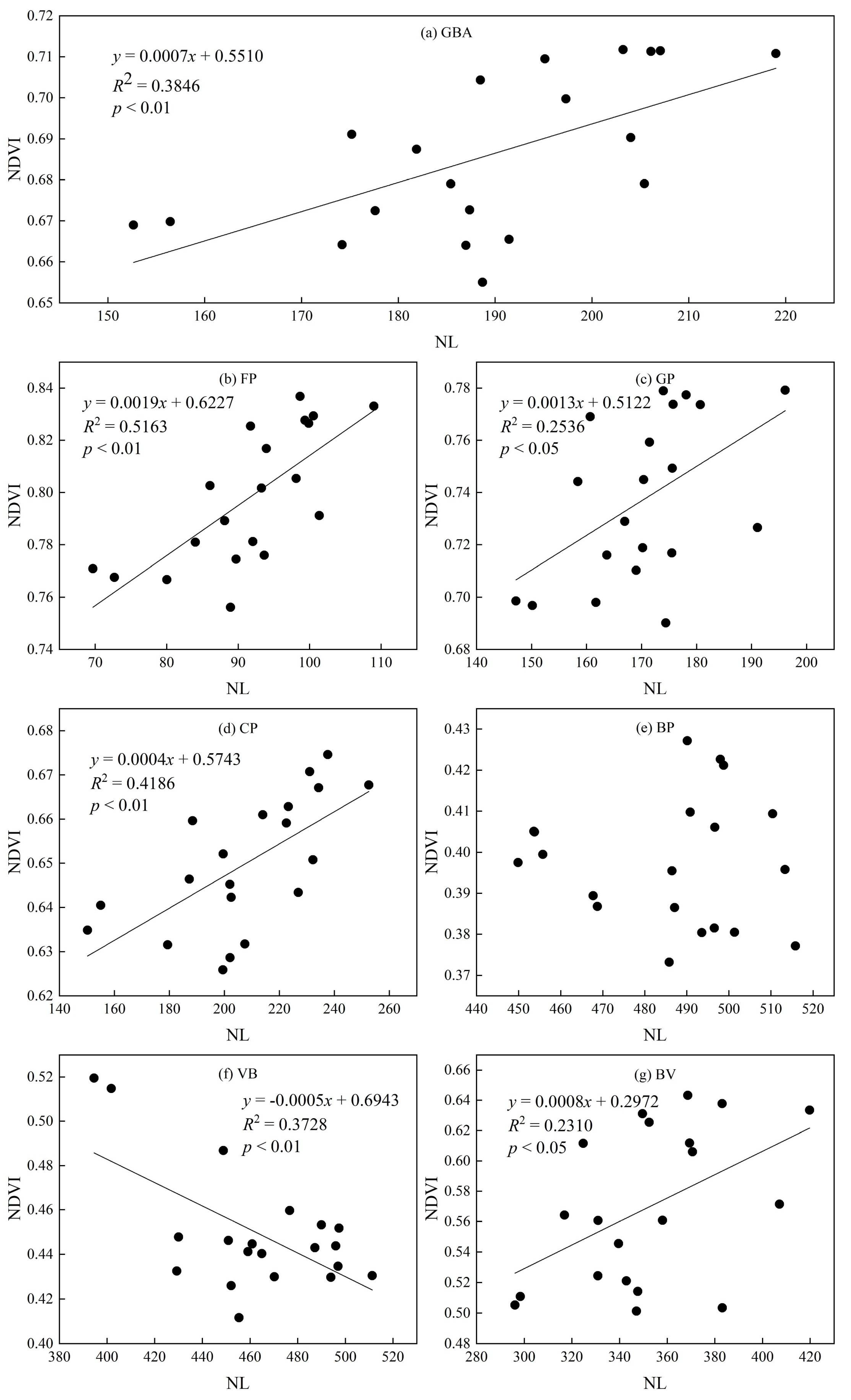
2.3.5. Correlation Analysis

In order to disentangle the relationships between vegetation dynamics and socioeconomic development, Pearson correlation analysis was performed via software Origin 2018 and the correlation coefficient (R) between the annual NDVI and the annual NL for different LUCC types was calculated based on the linear regression as follows:

$$R=\frac{{{\displaystyle \sum }}_{i=1}^n\left[\left(N{L}_i-\overline{NL}\right)\left(NDV{I}_i-\overline{NDVI}\right)\right]}{\sqrt{{{\displaystyle \sum }}_{i=1}^n{\left(N{L}_i-\overline{NL}\right)}^2{{\displaystyle \sum }}_{i=1}^n{\left(NDV{I}_i-\overline{NDVI}\right)}^2}}$$

(13)

where R is the correlation coefficient between NDVI and NL, NL_i and NDVI_i are the area-averaged NL and NDVI values of year i, $\overline{NL}$ and $\overline{NDVI}$ are the average NL and NDVI for the whole study period, and n is the number of years.

3. Results

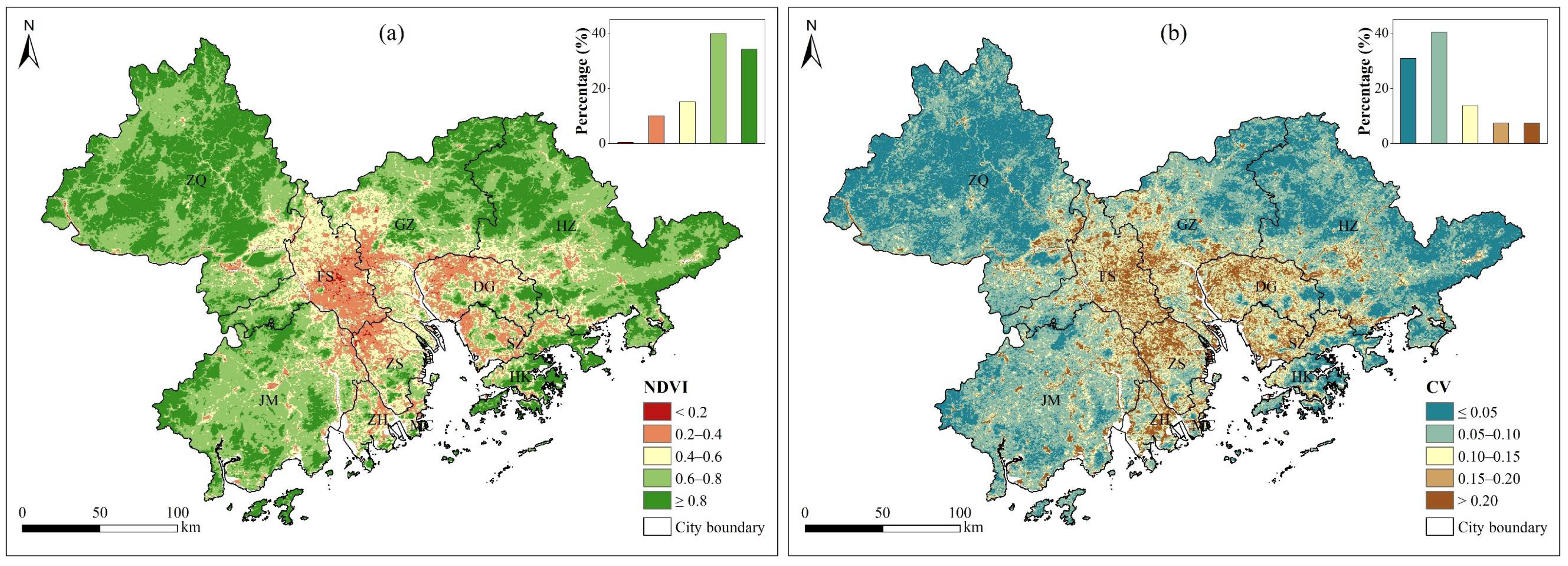
3.1. Spatial Heterogeneity and Fluctuations in Vegetation Dynamics

The NDVI averaged over the period 2001–2020 displayed a distinct spatial pattern: low values mainly distributed in the central region and high values in the peripheral region (Figure 2a). The NDVI was classified into five grades by an equal-interval classification method, and the area percentage was 0.53%, 10.09%, 15.26%, 39.92%, and 34.20% for each NDVI grade from low to high values. Regions with low NDVI values (NDVI < 0.4) were primarily distributed in the highly urbanized Pearl River Estuary including the southern GZ, FS, ZS, ZH, DG, SZ, and MC, while regions with high NDVI values (NDVI ≥ 0.6) were widely located in ZQ, HZ, JM, HK, and the northern GZ. Area statistics indicated that NDVI differentiated greatly across LUCC types (

Table 2. Area statistics of NDVI and CV for main LUCC types.

Variable 1	Grade	Area (%) of LUCC 2
		FP	GP	CP	BP	VB	BV
NDVI	<0.2	0	0.01	0.05	2.27	0.50	0
	0.2–0.4	0.17	0.43	4.94	57.12	36.64	3.45
	0.4–0.6	2.36	8.33	23.19	29.38	51.04	56.90
	0.6–0.8	37.67	63.38	67.59	11.07	11.58	39.65
	≥0.8	59.79	27.85	4.23	0.16	0.24	0
CV	≤0.05	49.00	23.00	15.77	1.63	0.41	0
	0.05–0.10	43.18	57.91	56.09	17.26	8.20	13.79
	0.10–0.15	6.07	13.81	17.42	36.26	27.36	51.72
	0.15–0.20	1.29	3.66	6.37	28.52	27.41	15.52
	>0.20	0.46	1.62	4.35	16.33	36.62	18.97

¹ NDVI—normalized difference vegetation index; CV—coefficient of variation. ² LUCC types: forest persistence (FP), grassland persistence (GP), cropland persistence (CP), built-up persistence (BP), vegetation to built-up (VB), and built-up to vegetation (BV).

). High NDVI values (NDVI ≥ 0.6) accounted for 97.47%, 91.23%, and 71.82% of FP, GP, and CP regions, respectively. Overall, NDVI for most vegetated areas was higher than 0.6, whereas the NDVI decreased significantly when vegetation changed to built-up with 88.18% of the VB region having NDVI lower than 0.6. In comparison, nearly 60% of the BP region had low NDVI values (NDVI < 0.4), but this percentage sharply decreased if built-up converted to vegetation.

The coefficient of variation (CV) of the NDVI time series had a highly similar spatial pattern to the averaged NDVI (Figure 2b). The CV was divided into five grades at an interval of 0.05 to depict vegetation fluctuations. Low fluctuations (71.30%) dominated most of the peripheral region with 30.95% for the CV ≤ 0.05 grade and 40.35% for the 0.05 < CV ≤ 0.10 grade. By contrast, vegetation in the central region generally had high fluctuations with CV > 0.15, which accounted for almost 15% of the study area. Vegetation fluctuations varied remarkably among LUCC types (Table 2). Forest showed the highest stability with nearly half of the FP region having the lowest fluctuations, followed by GP and CP regions. Most of the BP region experienced moderate to high fluctuations. In addition, changed regions between vegetation and built-up had relatively higher vegetation fluctuations than the unchanged regions, especially for the VB region with areas undergoing the highest fluctuations accounting for 36.62%.

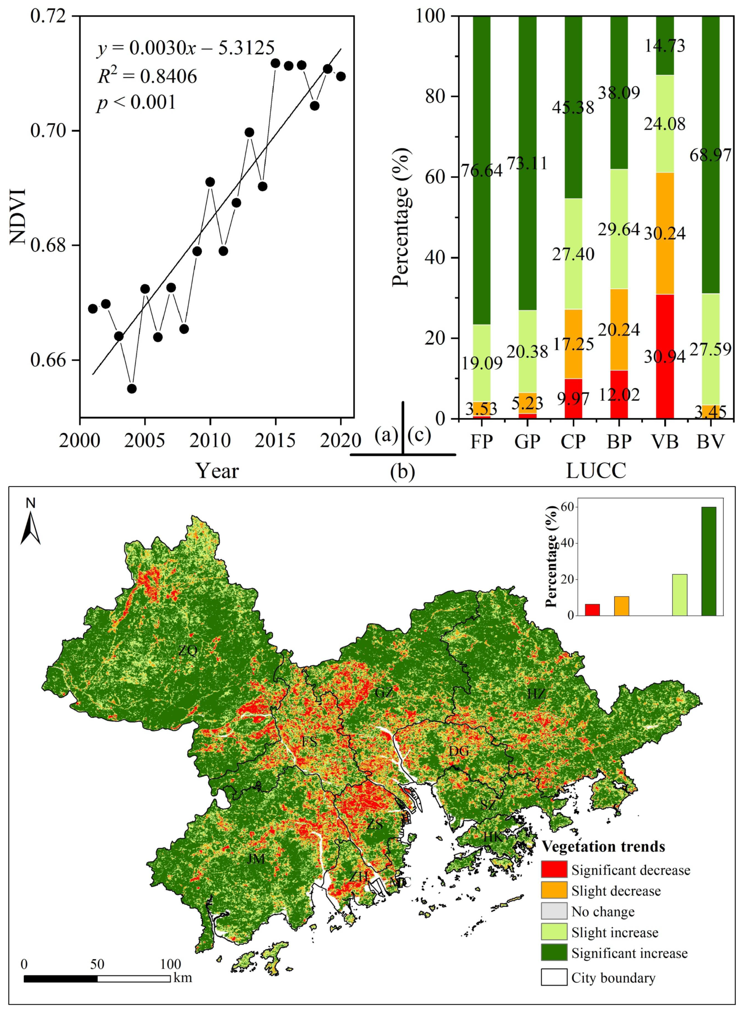
3.2. Trends in Vegetation Dynamics

At the regional scale, linear regression analysis showed that the area-averaged NDVI generally presented a significant increasing trend (p < 0.001, n = 20) at a rate of 0.0030 year⁻¹ during 2001–2020 (Figure 3a). The minimum value of the area-averaged NDVI was 0.6550 and the maximum value was 0.7117, which appeared in 2004 and 2015, respectively. At the pixel scale, the spatial pattern of NDVI trend over the past 20 years illustrated that NDVI increased in 82.99% of the study area, against 17.01% for the NDVI decreased area (Figure 3b). NDVI significantly increased over 60% of the study area, which was mainly distributed in ZC, HZ, JM, SZ, HK, and northern GZ. In contrast, areas with a significant decreasing trend were chiefly in FS, DG, SZ, ZH, and southern GZ, only accounting for 6.35% of the study area. Additionally, areas without vegetation change hardly existed (less than 0.01%).

Vegetation trends among main LUCC types demonstrated great differences (Figure 3c). Forest and grassland exhibited the largest area of significant increasing NDVI, covering 76.64% and 73.11% of FP and GP regions, much higher than other LUCC types. Areas with increasing NDVI could reach to approximately 70% for CP and BP regions, in which the significant increasing areas accounted for 45.38% and 38.09%, respectively. Instead, more than 60% (30.94% for significant decrease and 30.24% for slight decrease) of the VB region experienced an NDVI decrease, while an NDVI increase was observed over 96% (68.97% for significant increase and 27.59% for slight increase) of the BV region, even higher than FP and GP regions.

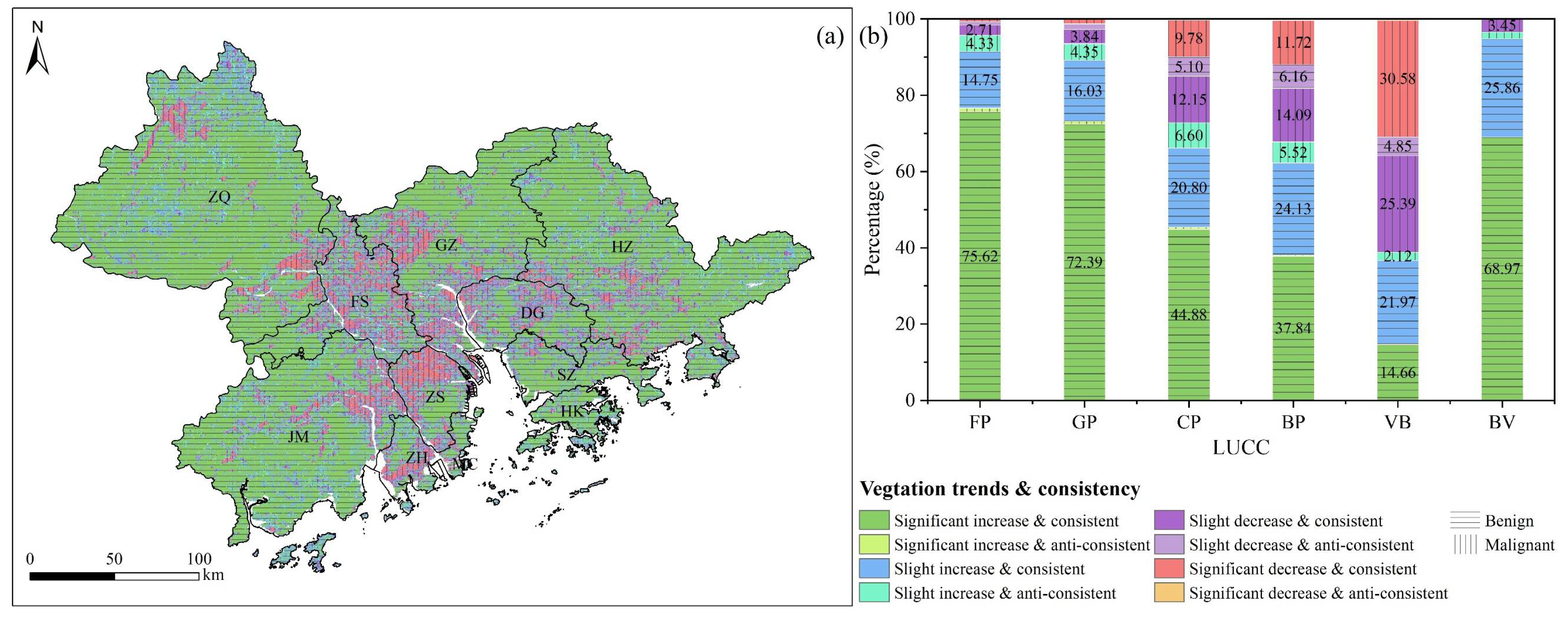
3.3. Future Changes in Vegetation Dynamics

The Hurst exponent analysis indicated that the future dynamics of NDVI in most of the study area would continue to keep the same change trend as the past 20 years (

Table 3. Future changes in NDVI based on trend analysis and Hurst exponent.

Trend Analysis		Hurst Exponent	Future Development		Area Percentage (%)
SNDVI	Z	H	Trend and Consistency	Direction
SNDVI > 0	|Z| > 1.96	0.5 < H < 1	Significant increase and consistent	Benign	59.28	80.06
SNDVI > 0	|Z| ≤ 1.96	0.5 < H < 1	Slight increase and consistent		17.93
SNDVI < 0	|Z| ≤ 1.96	0 < H < 0.5	Slight decrease and anti-consistent		2.74
SNDVI < 0	|Z| > 1.96	0 < H < 0.5	Significant decrease and anti-consistent		0.11
SNDVI > 0	|Z| > 1.96	0 < H < 0.5	Significant increase and anti-consistent	Malignant	0.74	19.94
SNDVI > 0	|Z| ≤ 1.96	0 < H < 0.5	Slight increase and anti-consistent		5.04
SNDVI < 0	|Z| ≤ 1.96	0.5 < H < 1	Slight decrease and consistent		7.91
SNDVI < 0	|Z| > 1.96	0.5 < H < 1	Significant decrease and consistent		6.25

, Figure 4a). Areas with a consistent NDVI trend (0.5 < H < 1) occupied 91.37% of the region, compared to areas with the anti-consistent trend (0 < H < 0.5) accounting for merely 8.63%. On the basis of the trend analysis and the Hurst exponent, the future development of NDVI was summarized as eight states, which could be concluded as two main directions: benign and malignant (Table 3). The consistent significant increasing trend was the most important state of future NDVI change, accounting for 59.28% of the study area, followed by the consistent slight increasing trend (17.93%). Together with the small area of anti-consistent decreasing trends, the percentage of areas where NDVI was predicted to develop in the benign direction as a whole reached 80.06%, over four times that in the malignant direction (19.94%). NDVI in most of the areas with malignant development presented a continuous decreasing trend, including the slight decrease (7.91%) and the significant decrease (6.25%). Moreover, areas that were predicted to convert from an increasing trend to a decreasing trend covered 5.78% of the study area.

Future changes in NDVI among LUCC varied dramatically (Figure 4b). Except for the VB region, NDVI in most of the other regions was predicted to sustain a continuously increasing trend. Areas with a future persistent significant increasing trend accounted for 75.62% and 72.39% of FP and GP regions, respectively, followed closely by the BV region with an area proportion of 68.97%, much higher than that of other LUCC types. In addition, NDVI in 44.88% of the CP region and 37.84% of the BP region would continue to increase dramatically, while this percentage was only 14.66% for the VB region. On the contrary, the area proportion of NDVI with a consistent significant decreasing trend in the VB region was highest at 30.58%, and this percentage was 25.39% for the area with a consistent slight decreasing trend. Collectively, NDVI in approximately 90% of the FP and GP regions and 70% of the CP, BP, and BV regions was predicted to develop in a benign direction, while NDVI in more than half (58.15%) of the VB region would develop in a malignant direction in the future.

4. Discussion

4.1. Spatiotemporal Variations in Vegetation Dynamics

Vegetation dynamics over the past 20 years (2001–2020) in the GBA generally displayed a distinct spatial pattern: low coverage, high fluctuations, and decreasing trends in the center, and high coverage, low fluctuations, and increasing trends in the peripheral regions (Figure 2 and Figure 3b), in agreement with previous studies [20,46]. This pattern coincided with the topography from alluvial plains in the central estuary area to mountains around its periphery. Firstly, topography is one of the most important determinants of vegetation distribution due to its significant effect on hydrological processes [47], local hydrothermal conditions [7], and soil quality [48]. Thus, forests with high NDVI values are usually distributed in high-elevation mountainous zones. Secondly, human activities are closely related to topography [20]. As negative relationships are commonly observed between elevation/slope and human activities, the land use in the GBA has formed a spatial pattern of “built-up–cropland–forest” from low to high elevations and small to large slopes (Figure 1). Urban expansion and infrastructure construction will inevitably cause vegetation degradation, so high fluctuations and decreasing trends of vegetation change mainly happen at lower elevations and smaller slopes. Thus, it can be concluded that urbanization plays a pivotal role in forming the spatiotemporal patterns of vegetation coverage, fluctuations, and trends in the GBA.

This study found that vegetation at the regional scale exhibited a significant linear greening trend, in line with a previous study [20]. However, the increasing rate of NDVI in our results (0.0030 year⁻¹) was smaller than that in the previous work (0.0033 year⁻¹). This is possibly due to the difference in the study period. Our analyses were conducted over a longer time series (2001–2020) than the previous study (2000–2016), and the browning trend after 2015 would reduce the overall rate of vegetation greening. In addition, our findings also indicated that the majority (91.37%) of the study area would retain the same vegetation trend in the future, no matter the increasing trend or the decreasing trend (Table 3, Figure 4a). This high proportion of future consistency implied a relatively stable state of long-term dependence of the NDVI time series.

4.2. Vegetation Trends among LUCC Types

Rapid economic development has been lasting for several decades in the GBA urban agglomeration, and human activities were widely regarded as one of the main causes of vegetation change. The correlation coefficient (R) between NDVI and NL was used to explore the influences of socioeconomic development on vegetation growth during the past 20 years (Figure 5). For the whole GBA, NDVI was significantly correlated with NL (p < 0.01), and the positive slope indicated that socioeconomic development was generally beneficial for vegetation greening (Figure 5a), consistent with previous studies highlighting a positive correlation between vegetation and economic growth (GDP, population) [20]. However, the impacts of socioeconomic development on vegetation varied for different LUCC types. Except for the negative correlation for the VB region and no obvious correlation for the BP region between NDVI and NL, significantly positive relationships were observed for other LUCC types (Figure 5).

Urbanization was widely regarded as the principal cause of vegetation browning in the core areas of the GBA [26,49,50], which was also concluded by our results that the decreasing trend of NDVI appeared in 61.18% of the areas converted from various types of vegetation to built-up lands (i.e., the VB region) throughout 2001–2020 (Figure 3). Results of correlation analysis between NDVI and NL also confirmed that socioeconomic activities inhibited vegetation growth in the newly developed built-up areas (Figure 5f). However, it was worth noting that vegetation in most (67.73%) of the unchanged built-up areas (i.e., the BP region) presented a greening trend, contradicting the general knowledge that economic development and population growth result in vegetation degradation [51,52]. One possible explanation is the re-feeding of economy to ecology. Taking the most developed GZ and SZ as an example, vegetation of old urban districts in both cities generally showed a significant increasing trend although the NDVI values in these areas were relatively low, and the greening trend was predicted to continue in the future (Figure 4). These results agree with other studies that also observed urban greening in most built-up areas in GZ and SZ recently [53,54]. Nevertheless, not all cities experienced greening in the BP regions, and some cities even presented vegetation degradation in most of the BP region such as ZQ. This may be related to the developmental status of cities that urban environments in cities with higher levels of economy are more likely to have positive effects on indirect enhancement of vegetation growth [55]. The lack of an obvious correlation between NDVI and NL for the BP region also confirmed this complicated vegetation change with socioeconomic growth (Figure 5e). Thus, those highly developed cities (i.e., GZ and SZ) were more likely to implement more investment in urban greening and green development to meet the growing demand for urban human settlement environments [56,57]. This was also supported by a prior work that highlighted a “win–win” relationship between economic growth and vegetation improvement in all municipalities of the Pearl River Delta, especially in recent years [20]. Another reason is the remarkable urban heat island effect in the Pearl River Delta region, which was previously deduced to enhance vegetation productivity [28]. In addition, the fertilization effect of carbon dioxide and nitrogen deposition also contributes to vegetation greening [58,59], particularly in urban areas with intensive transport emissions. Recent studies concluded the general negative direct impacts (land cover transformation) and widespread positive indirect impacts (changes in environments) of urbanization on vegetation growth [27,55], which can also be supported by our findings that vegetation greening occurred in most unchanged urban areas (i.e., the BP region) and vegetation browning happened in most newly developed urban areas (i.e., the VB region). The phenomenon of vegetation improvement in urban cores and vegetation degradation in newly developed peripheries was also observed in other regions [60,61]. As such, vegetation responses to urbanization are highly complex.

The persistent vegetated areas over the past 20 years in the GBA manifested obvious vegetation greening and high future consistency (Figure 3 and Figure 4). For the FP and GP regions, vegetation improved in over 90% of their ranges, and most of them were statistically significant. This was believed to be highly related to the ecological restoration projects such as the Grain to Green Program and the Natural Forest Conservation Program [62,63]. Artificial afforestation and forest facilitation via these projects and other ecological policies were beneficial for vegetation improvement. The significantly positive relationships between NDVI and NL for the FP and GP regions also revealed that more attention would be paid and more investment would be implemented to these ecological projects to facilitate better vegetation restoration and environment improvement (Figure 5b,c). For example, free grain and cash payments were provided for farmers who returned their farmlands on steep topographic slopes or with low yields to forest and grassland via policies such as the transregional compensation for ecological conservation [64,65]. Furthermore, these ecological projects, implemented since 1998, have formed extensive young forests, and forest regrowth and succession might consistently contribute to vegetation greening in the future [6,66]. For the CP region, most areas also showed a significant or slight increasing trend, accounting for 45.38% and 27.40%, respectively. Agricultural intensifications such as multiple cropping, fertilizer usage, effective irrigation, and agricultural mechanization were regarded as the main reason for cropland greening [6,57,67]. Moreover, cropland reclamation also contributed considerably to vegetation enhancement. In conclusion, vegetation greening was commonly observed in the unchanged vegetated areas (i.e., the FP, GP, and CP regions) during the urbanization process (Figure 5b–d), and the area percentage of significant increase was ranked as FP > GP > CP (Figure 3). This was comparable to a previous study that found that the contribution rate to vegetation productivity improvement was highest in the unchanged forest, followed by unchanged grassland and farmland in the six provinces along the southeast coast of China (including the GBA) during 1982–2015 [30]. Environmental efficiency of urban agglomeration development could be evaluated by the slope of linear regression [51], and the steeper slope between NDVI and NL for the FP region indicated a lower cost of forest per unit of socioeconomic growth than the GP and CP regions. Nevertheless, vegetation browning was still detected in some regions and more attention should be paid to these regions to prevent further degradation. To sum up, vegetation dynamics in the GBA vary greatly among different LUCC types during urbanization due to diverse natural and human-induced causes.

4.3. Limitations and Uncertainties

Some limitations and uncertainties remain in this study. First, the sensitivity to the presence of short-range dependence may affect the reliability of the Hurst exponent due to the short time of the NDVI observation [16,43]. Second, the vegetation change is more likely to be complex and nonlinear under the influence of climate change and anthropogenic disturbance [68,69], which may have great impacts on the accuracy of the predictions for future consistency of vegetation trends. Moreover, the duration of the consistency of future vegetation trends cannot be estimated by the Hurst analysis [8]. Therefore, a longer period of vegetation dynamics should be deeply studied and the abrupt change in vegetation trends should be necessarily considered in the next work. Additionally, vegetation dynamics are sophisticated and influenced by multiple factors including climate change and human activities, and usually perform distinctively for different seasons [10,50,70], so future efforts are needed to reveal the underlying mechanisms with a finer temporal resolution.

5. Conclusions

This study evaluated the spatiotemporal heterogeneity, fluctuations, trends, and future consistency of vegetation dynamics by quantifying the coefficient of variation, Theil–Sen median trend analysis, and Hurst exponent of NDVI time series over the period 2001–2020 in the GBA, a rapidly developing urban agglomeration in South China. Results demonstrated that vegetation exhibited a significant greening trend at the regional scale during the past 20 years. Vegetation improvement generally appeared in the peripheral mountainous regions with relatively high NDVI values and low fluctuations, while vegetation degradation mainly happened in the central estuary area with relatively low NDVI values and high fluctuations. Future vegetation change in most areas will continue the existing trends, and 80.06% of the study area was predicted to develop in a benign direction, against 19.94% in a malignant direction. Vegetation dynamics among LUCC types varied remarkedly. The persistent forest and grassland contributed the most to vegetation greening with NDVI in over 90% of areas showing an increasing trend, as well as the regions converted from built-up to vegetation. Most of the persistent cropland and built-up land also presented vegetation enhancement but with a lower proportion at approximately 70%. Nevertheless, more than 60% of the regions converted from vegetation to built-up experienced vegetation degradation. Correlation analysis revealed that vegetation growth was positively correlated with socioeconomic development except for the persistent built-up areas and newly developed built-up areas. Multiple anthropogenic and natural factors were regarded as main reasons for these vegetation changes.

References

1. Zeng, Z.Z.; Piao, S.L.; Li, L.Z.X.; Wang, T.; Ciais, P.; Lian, X.; Yang, Y.T.; Mao, J.F.; Shi, X.Y.; Myneni, R.B. Impact of Earth Greening on the Terrestrial Water Cycle. J. Clim. 2018, 31, 2633–2650. [Google Scholar] [CrossRef]
2. De Carvalho, R.M.; Szlafsztein, C.F. Urban vegetation loss and ecosystem services: The influence on climate regulation and noise and air pollution. Environ. Pollut. 2019, 245, 844–852. [Google Scholar] [CrossRef] [PubMed]
3. Sakaguchi, K.; Zeng, X.; Leung, L.R.; Shao, P. Influence of dynamic vegetation on carbon-nitrogen cycle feedback in the Community Land Model (CLM4). Environ. Res. Lett. 2016, 11, 124029. [Google Scholar] [CrossRef]
4. Feng, H.H.; Zou, B.; Luo, J.H. Coverage-dependent amplifiers of vegetation change on global water cycle dynamics. J. Hydrol. 2017, 550, 220–229. [Google Scholar] [CrossRef]
5. Port, U.; Brovkin, V.; Claussen, M. The influence of vegetation dynamics on anthropogenic climate change. Earth Syst. Dynam. 2012, 3, 233–243. [Google Scholar] [CrossRef]
6. Piao, S.L.; Wang, X.H.; Park, T.; Chen, C.; Lian, X.; He, Y.; Bjerke, J.W.; Chen, A.P.; Ciais, P.; Tommervik, H.; et al. Characteristics, drivers and feedbacks of global greening. Nat. Rev. Earth Env. 2020, 1, 14–27. [Google Scholar] [CrossRef]
7. Peng, J.; Liu, Z.H.; Liu, Y.H.; Wu, J.S.; Han, Y.A. Trend analysis of vegetation dynamics in Qinghai-Tibet Plateau using Hurst Exponent. Ecol. Indic. 2012, 14, 28–39. [Google Scholar] [CrossRef]
8. Jiang, W.G.; Yuan, L.H.; Wang, W.J.; Cao, R.; Zhang, Y.F.; Shen, W.M. Spatio-temporal analysis of vegetation variation in the Yellow River Basin. Ecol. Indic. 2015, 51, 117–126. [Google Scholar] [CrossRef]
9. Wu, X.X.; Lv, M.; Jin, Z.Y.; Michishita, R.; Chen, J.; Tian, H.Y.; Tu, X.B.; Zhao, H.M.; Niu, Z.G.; Chen, X.L.; et al. Normalized difference vegetation index dynamic and spatiotemporal distribution of migratory birds in the Poyang Lake wetland, China. Ecol. Indic. 2014, 47, 219–230. [Google Scholar] [CrossRef]
10. Sarmah, S.; Jia, G.S.; Zhang, A.Z. Satellite view of seasonal greenness trends and controls in South Asia. Environ. Res. Lett. 2018, 13, 034026. [Google Scholar] [CrossRef]
11. Dubovyk, O.; Landmann, T.; Erasmus, B.F.N.; Tewes, A.; Schellberg, J. Monitoring vegetation dynamics with medium resolution MODIS-EVI time series at sub-regional scale in southern Africa. Int. J. Appl. Earth Obs. Geoinf. 2015, 38, 175–183. [Google Scholar] [CrossRef]
12. Zhao, L.; Dai, A.G.; Dong, B. Changes in global vegetation activity and its driving factors during 1982-2013. Agric. For. Meteorol. 2018, 249, 198–209. [Google Scholar] [CrossRef]
13. Gutman, G.; Ignatov, A. The derivation of the green vegetation fraction from NOAA/AVHRR data for use in numerical weather prediction models. Int. J. Remote Sens. 1998, 19, 1533–1543. [Google Scholar] [CrossRef]
14. Guay, K.C.; Beck, P.S.A.; Berner, L.T.; Goetz, S.J.; Baccini, A.; Buermann, W. Vegetation productivity patterns at high northern latitudes: A multi-sensor satellite data assessment. Glob. Change Biol. 2014, 20, 3147–3158. [Google Scholar] [CrossRef]
15. Tucker, C.J. Red and photographic infrared linear combinations for monitoring vegetation. Remote Sens. Environ. 1979, 8, 127–150. [Google Scholar] [CrossRef]
16. Li, J.; Wang, J.L.; Zhang, J.; Zhang, J.P.; Kong, H. Dynamic changes of vegetation coverage in China-Myanmar economic corridor over the past 20 years. Int. J. Appl. Earth Obs. Geoinf. 2021, 102, 102378. [Google Scholar] [CrossRef]
17. Ruan, Z.; Kuang, Y.Q.; He, Y.Y.; Zhen, W.; Ding, S. Detecting Vegetation Change in the Pearl River Delta Region Based on Time Series Segmentation and Residual Trend Analysis (TSS-RESTREND) and MODIS NDVI. Remote Sens. 2020, 12, 4049. [Google Scholar] [CrossRef]
18. Chen, C.; He, B.; Yuan, W.P.; Guo, L.L.; Zhang, Y.F. Increasing interannual variability of global vegetation greenness. Environ. Res. Lett. 2019, 14, 124005. [Google Scholar] [CrossRef]
19. Fensholt, R.; Langanke, T.; Rasmussen, K.; Reenberg, A.; Prince, S.D.; Tucker, C.; Scholes, R.J.; Le, Q.B.; Bondeau, A.; Eastman, R.; et al. Greenness in semi-arid areas across the globe 1981-2007 - an Earth Observing Satellite based analysis of trends and drivers. Remote Sens. Environ. 2012, 121, 144–158. [Google Scholar] [CrossRef]
20. Hu, M.M.; Xia, B.C. A significant increase in the normalized difference vegetation index during the rapid economic development in the Pearl River Delta of China. Land Degrad. Dev. 2019, 30, 359–370. [Google Scholar] [CrossRef]
21. Tran, T.V.; Tran, D.X.; Nguyen, H.; Latorre-Carmona, P.; Myint, S.W. Characterising spatiotemporal vegetation variations using LANDSAT time-series and Hurst exponent index in the Mekong River Delta. Land Degrad. Dev. 2021, 32, 3507–3523. [Google Scholar] [CrossRef]
22. Ndayisaba, F.; Guo, H.; Bao, A.M.; Guo, H.; Karamage, F.; Kayiranga, A. Understanding the Spatial Temporal Vegetation Dynamics in Rwanda. Remote Sens. 2016, 8, 129. [Google Scholar] [CrossRef]
23. Detsch, F.; Otte, I.; Appelhans, T.; Hemp, A.; Nauss, T. Seasonal and long-term vegetation dynamics from 1-km GIMMS-based NDVI time series at Mt. Kilimanjaro, Tanzania. Remote Sens. Environ. 2016, 178, 70–83. [Google Scholar] [CrossRef]
24. Yuan, J.; Xu, Y.P.; Xiang, J.; Wu, L.; Wang, D.Q. Spatiotemporal variation of vegetation coverage and its associated influence factor analysis in the Yangtze River Delta, eastern China. Environ. Sci. Pollut. R 2019, 26, 32866–32879. [Google Scholar] [CrossRef] [PubMed]
25. Imhoff, M.L.; Bounoua, L.; DeFries, R.; Lawrence, W.T.; Stutzer, D.; Tucker, C.J.; Ricketts, T. The consequences of urban land transformation on net primary productivity in the United States. Remote Sens. Environ. 2004, 89, 434–443. [Google Scholar] [CrossRef]
26. Du, J.Q.; Quan, Z.J.; Fang, S.F.; Liu, C.C.; Wu, J.H.; Fu, Q. Spatiotemporal changes in vegetation coverage and its causes in China since the Chinese economic reform. Environ. Sci. Pollut. R 2020, 27, 1144–1159. [Google Scholar] [CrossRef] [PubMed]
27. Zhao, S.Q.; Liu, S.G.; Zhou, D.C. Prevalent vegetation growth enhancement in urban environment. Proc. Natl. Acad. Sci. USA 2016, 113, 6313–6318. [Google Scholar] [CrossRef] [PubMed]
28. Pei, F.S.; Li, X.; Liu, X.P.; Wang, S.J.; He, Z.J. Assessing the differences in net primary productivity between pre- and post-urban land development in China. Agric. For. Meteorol. 2013, 171, 174–186. [Google Scholar] [CrossRef]
29. Gregg, J.W.; Jones, C.G.; Dawson, T.E. Urbanization effects on tree growth in the vicinity of New York City. Nature 2003, 424, 183–187. [Google Scholar] [CrossRef] [PubMed]
30. Xue, P.; Liu, H.Y.; Zhang, M.Y.; Gong, H.B.; Cao, L. Nonlinear Characteristics of NPP Based on Ensemble Empirical Mode Decomposition from 1982 to 2015-A Case Study of Six Coastal Provinces in Southeast China. Remote Sens. 2022, 14, 15. [Google Scholar] [CrossRef]
31. Taubenböck, H.; Weigand, M.; Esch, T.; Staab, J.; Wurm, M.; Mast, J.; Dech, S. A new ranking of the world’s largest cities-Do administrative units obscure morphological realities? Remote Sens. Environ. 2019, 232, 111353. [Google Scholar] [CrossRef]
32. Ma, Y.L.; Zhang, S.H.; Yang, K.; Li, M.C. Influence of spatiotemporal pattern changes of impervious surface of urban megaregion on thermal environment: A case study of the Guangdong-Hong Kong-Macao Greater Bay Area of China. Ecol. Indic. 2021, 121, 107106. [Google Scholar] [CrossRef]
33. Lan, S.X.; Dong, Z.J. Incorporating Vegetation Type Transformation with NDVI Time-Series to Study the Vegetation Dynamics in Xinjiang. Sustainability 2022, 14, 582. [Google Scholar] [CrossRef]
34. Jiang, C.; Wu, Z.F.; Cheng, J.; Yu, Q.; Rao, X.Q. Impacts of urbanization on net primary productivity in the Pearl River Delta, China. Int. J. Plant Prod. 2015, 9, 581–598. [Google Scholar]
35. Yan, Y.C.; Liu, X.P.; Wang, F.Y.; Li, X.; Ou, J.P.; Wen, Y.Y.; Liang, X. Assessing the impacts of urban sprawl on net primary productivity using fusion of Landsat and MODIS data. Sci. Total Environ. 2018, 613, 1417–1429. [Google Scholar] [CrossRef] [PubMed]
36. Hu, M.M.; Li, Z.T.; Wang, Y.F.; Jiao, M.Y.; Li, M.; Xia, B.C. Spatio-temporal changes in ecosystem service value in response to land-use/cover changes in the Pearl River Delta. Resour. Conserv. Recycl. 2019, 149, 106–114. [Google Scholar] [CrossRef]
37. Jonsson, P.; Eklundh, L. TIMESAT - a program for analyzing time-series of satellite sensor data. Comput. Geosci. 2004, 30, 833–845. [Google Scholar] [CrossRef]
38. Zhang, L.X.; Ren, Z.H.; Chen, B.; Gong, P.; Fu, H.H.; Xu, B. A Prolonged Artificial Nighttime-light Dataset of China (1984–2020). 2021. [Google Scholar] [CrossRef]
39. Sen, P.K. Estimates of the Regression Coefficient Based on Kendall’s Tau. J. Am. Stat. Assoc. 1968, 63, 1379–1389. [Google Scholar] [CrossRef]
40. Theil, H. A Rank-Invariant Method of Linear and Polynomial Regression Analysis I, II, and III. Proc. K. Ned. Akad. Wet. 1950, 53, 386–392, 521–525, 1397–1412. [Google Scholar] [CrossRef]
41. Kendall, M. Rank Correlation Methods; Charles Griffin: London, UK, 1975. [Google Scholar]
42. Hurst, H.E. Long-Term Storage Capacity of Reservoirs. Trans. Am. Soc. Civ. Eng. 1951, 116, 770–799. [Google Scholar] [CrossRef]
43. Barunik, J.; Kristoufek, L. On Hurst exponent estimation under heavy-tailed distributions. Physica A 2010, 389, 3844–3855. [Google Scholar] [CrossRef]
44. Xu, F.; Zhou, Y.Y.; Zhao, L.L. Spatial and temporal variability in extreme precipitation in the Pearl River Basin, China from 1960 to 2018. Int. J. Climatol. 2022, 42, 797–816. [Google Scholar] [CrossRef]
45. Liu, W.; Zhan, J.Y.; Zhao, F.; Yan, H.M.; Zhang, F.; Wei, X.Q. Impacts of urbanization-induced land-use changes on ecosystem services: A case study of the Pearl River Delta Metropolitan Region, China. Ecol. Indic. 2019, 98, 228–238. [Google Scholar] [CrossRef]
46. Zhang, Y.H.; Ye, A.Z. Quantitatively distinguishing the impact of climate change and human activities on vegetation in mainland China with the improved residual method. Gisci. Remote Sens. 2021, 58, 235–260. [Google Scholar] [CrossRef]
47. Moore, I.D.; Grayson, R.B.; Ladson, A.R. Digital Terrain Modeling—a Review of Hydrological, Geomorphological, and Biological Applications. Hydrol. Process. 1991, 5, 3–30. [Google Scholar] [CrossRef]
48. Geng, S.B.; Shi, P.L.; Zong, N.; Zhu, W.R. Using soil survey database to assess soil quality in the heterogeneous Taihang Mountains, north China. Sustainability 2018, 10, 3443. [Google Scholar] [CrossRef]
49. Qiu, B.W.; Li, W.J.; Zhong, M.; Tang, Z.H.; Chen, C.C. Spatiotemporal analysis of vegetation variability and its relationship with climate change in China. Geo Spat. Inf. Sci. 2014, 17, 170–180. [Google Scholar] [CrossRef]
50. Wu, Y.Z.; Tang, G.P.; Gua, H.; Liu, Y.L.; Yang, M.Z.; Sun, L. The variation of vegetation greenness and underlying mechanisms in Guangdong province of China during 2001-2013 based on MODIS data. Sci. Total Environ. 2019, 653, 536–546. [Google Scholar] [CrossRef]
51. Liu, H.X.; Han, B.L.; Wang, L. Modeling the spatial relationship between urban ecological resources and the economy. J. Clean Prod. 2018, 173, 207–216. [Google Scholar] [CrossRef]
52. Shipigina, E.; Rees, W.G. Analysis of human impact on boreal vegetation around Monchegorsk, Kola peninsula, using automated remote sensing technique. Polar. Rec. 2012, 48, 94–106. [Google Scholar] [CrossRef]
53. Yu, W.J.; Zhou, W.Q.; Dawa, Z.; Wang, J.; Qian, Y.G.; Wang, W.M. Quantifying Urban Vegetation Dynamics from a Process Perspective Using Temporally Dense Landsat Imagery. Remote Sens. 2021, 13, 3217. [Google Scholar] [CrossRef]
54. Zhu, Z.; Fu, Y.C.; Woodcock, C.E.; Olofsson, P.; Vogelmann, J.E.; Holden, C.; Wang, M.; Dai, S.; Yu, Y. Including land cover change in analysis of greenness trends using all available Landsat 5, 7, and 8 images: A case study from Guangzhou, China (2000–2014). Remote Sens. Environ. 2016, 185, 243–257. [Google Scholar] [CrossRef]
55. Zhang, L.; Yang, L.; Zohner, C.M.; Crowther, T.W.; Li, M.C.; Shen, F.X.; Guo, M.; Qin, J.; Yao, L.; Zhou, C.H. Direct and indirect impacts of urbanization on vegetation growth across the world’s cities. Sci. Adv. 2022, 8, eabo0095. [Google Scholar] [CrossRef]
56. Wang, M.X.; Zhao, H.H.; Cui, J.X.; Fan, D.; Lv, B.; Wang, G.; Li, Z.H.; Zhou, G.J. Evaluating green development level of nine cities within the Pearl River Delta, China. J. Clean Prod. 2018, 174, 315–323. [Google Scholar] [CrossRef]
57. Feng, D.R.; Bao, W.K.; Yang, Y.Y.; Fu, M.C. How do government policies promote greening? Evidence from China. Land Use Pol. 2021, 104, 105389. [Google Scholar] [CrossRef]
58. Los, S.O. Analysis of trends in fused AVHRR and MODIS NDVI data for 1982-2006: Indication for a CO2 fertilization effect in global vegetation. Glob. Biogeochem. Cy. 2013, 27, 318–330. [Google Scholar] [CrossRef]
59. Greaver, T.L.; Clark, C.M.; Compton, J.E.; Vallano, D.; Talhelm, A.F.; Weaver, C.P.; Band, L.E.; Baron, J.S.; Davidson, E.A.; Tague, C.L.; et al. Key ecological responses to nitrogen are altered by climate change. Nat. Clim. Change 2016, 6, 836–843. [Google Scholar] [CrossRef]
60. de la Barrera, F.; Henriquez, C. Vegetation cover change in growing urban agglomerations in Chile. Ecol. Indic. 2017, 81, 265–273. [Google Scholar] [CrossRef]
61. Esau, I.; Miles, V.V.; Davy, R.; Miles, M.W.; Kurchatova, A. Trends in normalized difference vegetation index (NDVI) associated with urban development in northern West Siberia. Atmos. Chem. Phys. 2016, 16, 9563–9577. [Google Scholar] [CrossRef]
62. Liu, J.G.; Li, S.X.; Ouyang, Z.Y.; Tam, C.; Chen, X.D. Ecological and socioeconomic effects of China’s policies for ecosystem services. Proc. Natl. Acad. Sci. USA 2008, 105, 9477–9482. [Google Scholar] [CrossRef]
63. Huang, Y.S.; Li, P.; An, Q.; Mao, F.J.; Zhai, W.C.; Yu, K.F.; He, Y.L. Long-term land use/cover changes reduce soil erosion in an ionic rare-earth mineral area of southern China. Land Degrad. Dev. 2021, 32, 4042–4055. [Google Scholar] [CrossRef]
64. Cao, R.F.; Zhang, A.L.; Wen, L.J. Trans-regional compensation mechanism under imbalanced land development: From the local government economic welfare perspective. Habitat Int. 2018, 77, 56–63. [Google Scholar] [CrossRef]
65. Shang, W.X.; Gong, Y.C.; Wang, Z.J.; Stewardson, M.J. Eco-compensation in China: Theory, practices and suggestions for the future. J. Environ. Manage. 2018, 210, 162–170. [Google Scholar] [CrossRef]
66. Zhang, Y.; Yao, Y.T.; Wang, X.H.; Liu, Y.W.; Piao, S.L. Mapping spatial distribution of forest age in China. Earth Space Sci. 2017, 4, 108–116. [Google Scholar] [CrossRef]
67. Chen, C.; Park, T.; Wang, X.H.; Piao, S.L.; Xu, B.D.; Chaturvedi, R.K.; Fuchs, R.; Brovkin, V.; Ciais, P.; Fensholt, R.; et al. China and India lead in greening of the world through land-use management. Nat. Sustain. 2019, 2, 122–129. [Google Scholar] [CrossRef] [PubMed]
68. Liu, Y.X.; Wang, Y.L.; Du, Y.Y.; Zhao, M.Y.; Peng, J. The application of polynomial analyses to detect global vegetation dynamics during 1982-2012. Int. J. Remote Sens. 2016, 37, 1568–1584. [Google Scholar] [CrossRef]
69. Fang, X.Q.; Zhu, Q.A.; Ren, L.L.; Chen, H.; Wang, K.; Peng, C.H. Large-scale detection of vegetation dynamics and their potential drivers using MODIS images and BFAST: A case study in Quebec, Canada. Remote Sens. Environ. 2018, 206, 391–402. [Google Scholar] [CrossRef]
70. Chu, H.S.; Venevsky, S.; Wu, C.; Wang, M.H. NDVI-based vegetation dynamics and its response to climate changes at Amur-Heilongjiang River Basin from 1982 to 2015. Sci. Total Environ. 2019, 650, 2051–2062. [Google Scholar] [CrossRef]
Figure 1. Land use/land cover (LULC) maps of the Guangdong–Hong Kong–Macao Greater Bay Area (GBA) in 2000 (a) and 2020 (b).
Remotesensing 14 03993 g001
Figure 2. Spatial distribution of NDVI (a) and CV (b) in the GBA during 2001–2020. NDVI—normalized difference vegetation index; CV—coefficient of variation.
Remotesensing 14 03993 g002
Figure 3. Trends of inter-annual NDVI in the GBA from 2001 to 2020. (a) The area-averaged NDVI trend; (b) the spatial pattern of NDVI trend; (c) the area percentage of NDVI trend for main LUCC types. FP—forest persistence; GP—grassland persistence; CP—cropland persistence; BP—built-up persistence; VB—vegetation to built-up; BV—built-up to vegetation.
Remotesensing 14 03993 g003
Figure 4. Future trends of NDVI in the GBA. (a) Spatial pattern of NDVI trend and future consistency; (b) area percentage of NDVI future trends for main LUCC types. FP—forest persistence; GP—grassland persistence; CP—cropland persistence; BP—built-up persistence; VB—vegetation to built-up; BV—built-up to vegetation.
Remotesensing 14 03993 g004
Figure 5. Correlations of NDVI and NL for the period 2001–2020. (a) Linear regression between NDVI and NL for the whole GBA; (bg) linear regression between NDVI and NL across different LUCC types. NL—night light; FP—forest persistence; GP—grassland persistence; CP—cropland persistence; BP—built-up persistence; VB—vegetation to built-up; BV—built-up to vegetation.
Remotesensing 14 03993 g005