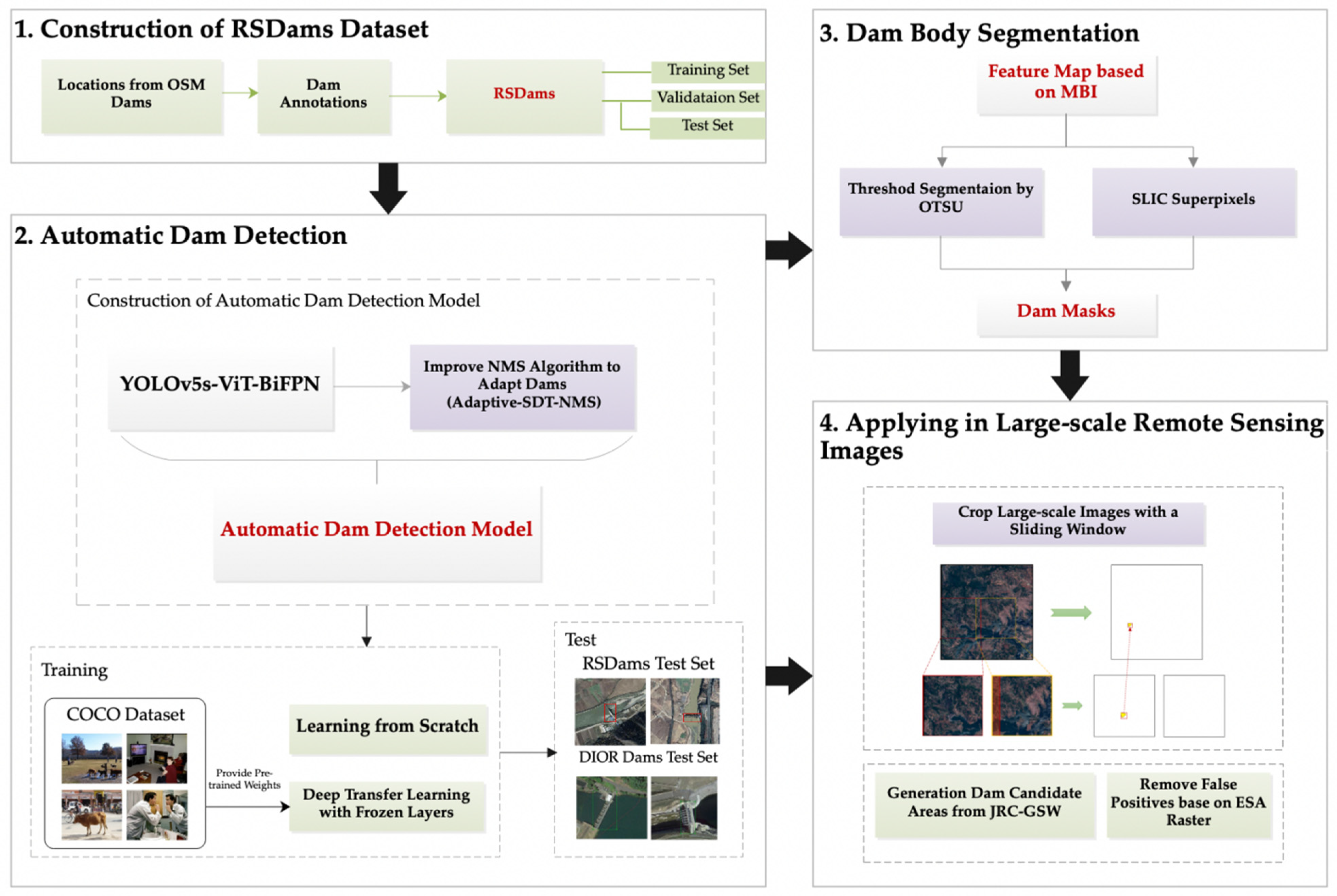
Article

Dam Extraction from High-Resolution Satellite Images Combined with Location Based on Deep Transfer Learning and Post-Segmentation with an Improved MBI

1
Aerospace Information Research Institute, Chinese Academy of Sciences, Beijing 100101, China
2
University of Chinese Academy of Sciences, Beijing 100049, China
*
Author to whom correspondence should be addressed.
These authors contributed equally to this work.
Remote Sens. 2022, 14(16), 4049; https://doi.org/10.3390/rs14164049
Submission received: 28 June 2022 / Revised: 9 August 2022 / Accepted: 16 August 2022 / Published: 19 August 2022
(This article belongs to the Special Issue Information Retrieval from Remote Sensing Images)

Abstract

:
Accurate mapping of dams can provide useful information about geographical locations and boundaries and can help improve public dam datasets. However, when applied to disaster emergency management, it is often difficult to completely determine the distribution of dams due to the incompleteness of the available data. Thus, we propose an automatic and intelligent extraction method that combines location with post-segmentation for dam detection. First, we constructed a dataset named RSDams and proposed an object detection model, YOLOv5s-ViT-BiFPN (You Only Look Once version 5s-Vision Transformer-Bi-Directional Feature Pyramid Network), with a training method using deep transfer learning to generate graphical locations for dams. After retraining the model on the RSDams dataset, its precision for dam detection reached 88.2% and showed a 3.4% improvement over learning from scratch. Second, based on the graphical locations, we utilized an improved Morphological Building Index (MBI) algorithm for dam segmentation to derive dam masks. The average overall accuracy and Kappa coefficient of the model applied to 100 images reached 97.4% and 0.7, respectively. Finally, we applied the dam extraction method to two study areas, namely, Yangbi County of Yunnan Province and Changping District of Beijing in China, and the recall rates reached 69.2% and 81.5%, respectively. The results show that our method has high accuracy and good potential to serve as an automatic and intelligent method for the establishment of a public dam dataset on a regional or national scale.

1. Introduction

Dams are barriers to rivers or streams used to impound water for the construction of reservoirs or to head up water levels. There are various purposes for the construction of dams, including the generation of hydroelectricity, flood mitigation, irrigation, water supply, and navigation [1]. Accurate mapping of dams can provide useful information regarding geographical locations and boundaries for safety management. Currently, several global datasets for dams exist, such as the Global Reservoir and Dam database (GRanD) [1], AQUASTAT from the FAO’s Global Information System on Water and Agriculture [2], Future Hydropower Reservoirs and Dams (FHReD) [3], the Global Georeferenced Database of Dams (GOODD) [4], OpenStreetMap (OSM) Dams [5], and the International Commission on Large Dams (ICOLD) [6]. These were mostly collected from existing databases, national archives, news from the Internet or images from Google Earth. However, for realistic needs, such as disaster emergency management, these datasets are deficient when it comes to data sharing; they also lack information regarding medium or small dams and contain unreliable location or boundary information for dams.
Remote sensing satellite technology should function despite geographic restrictions, which makes it possible to detect dams in any region. Therefore, developing a means by which to detect dams automatically and intelligently from high-resolution satellite images with high accuracy is both a challenge and a requirement for dam dataset updates. Deep learning is one of the most used artificial intelligent technologies and has been utilized in many fields, such as medical diagnosis, voice recognition, and image identification. There has already been some research on dam detection using deep learning methods. For example, Balaniuk et al. [7] used Fully Convolutional Networks (FCN) [8] to classify 263 non-registered tailing dams in Brazil. SSD (Single Shot MultiBox Detector) [9] and YOLO (You Only Look Once) [10] are the most popular series of one-stage object detection models that have been successfully applied in dam detection [11,12,13,14] with high accuracy. With regard to the types of dams, most research has focused on tailing dams [7,11,13], while there has been little focus on other types [12,14].
Notably, deep learning is an unsupervised or semi-supervised feature learning method that requires a large amount of data [15]. Its traditional training method is to construct different models according to different targets. However, there are some conflicts that deep learning methods cannot solve. For example, conflicts often exist between the rapid growth of big data and the limited availability of labeled data, massive training data and low computing power, generic descriptors and specific tasks [16,17].
Transfer learning can save computational and time resources and improve the generalization performance and robustness of deep learning methods with limited data by using knowledge from large-scale annotated open datasets [16,17,18]. Deep transfer learning employs this strategy in the training process of deep learning, which has great potential to solve the above conflicts [15].
Computer vision problems can be categorized as image classification when the goal is to judge whether the target object exists in an image, object detection when the goal is to classify and detect the target object by bounding boxes, and object segmentation when the goal is to generate masks of the target object in an image [7]. Current studies mostly focus on locating or displaying the positions of dams with bounding boxes. Because dams are sparsely distributed targets, it is not easy to segment them out of their complicated backgrounds with small errors in high-resolution remote sensing imagery. However, clear edges of dams are necessary for the construction and updating of datasets. Therefore, we used a post-segmentation method to provide informative masks within the bounding boxes of dams generated by an object detection model.
As a crucial manmade object, dams are similar to buildings in optical images in that they present higher reflectance than that of their periphery and are also built with similar concrete materials. Hence, building segmentation algorithms can be used to generate masks for dams. The Morphological Building Index (MBI) [19] was used to automatically extract buildings from high-resolution images. The basic idea of the MBI is based on the low spatial variation within the building’s body and the high variation at the edge, which represents the brightness, contrast, size, and directionality characteristics of buildings with a series of morphological operators [20]. When applying MBI, four thresholds, namely, the MBI, NDVI, the length–width ratio, and the area, are used to extract buildings manually from MBI feature images [19,20]. OTSU [21] is an adaptive threshold algorithm that has been used to help automatically detect buildings from the background [22]. Moreover, there is noise within buildings. The Simple Linear Iterative Cluster (SLIC) algorithm [23] is a segmentation algorithm that can generate superpixels and accurate homogeneous boundaries. To remove noise in building images, Wei et al. proposed [24] an approach that combines MBI and SLIC, which can remove small noise in building binary maps. Given these points, we attempted to introduce an improved MBI into dam segmentation within the bounding boxes of dams.
In this paper, we propose a method that extracts dams automatically and intelligently from high-resolution remote sensing satellite images. First, we exploited an object detection model using a training method with deep transfer learning to generate bounding boxes for dams. Second, we used an improved MBI to further extract the dam masks. Then, we illustrate the application of dam location and post-segmentation to high-resolution remote sensing satellite images.

2. Materials and Methods

In this study, we propose an automatic and intelligent extraction method for dams. This mainly consists of four parts, as shown in Figure 1: the construction of the RSDams dataset, automatic dam detection by YOLOv5s-ViT-BiFPN with a training method using deep transfer learning, dam segmentation, and application in high-resolution remote sensing images. The details are described in the following sections.

2.1. Study Areas and Satellite Data

The selected study areas were Yangbi County of Yunnan Province and the Changping District of Beijing in China, with areas of 1860 km2 and 1343.5 km2, respectively (Figure 2). Considering regional diversity, we selected these two study areas because one is a typical mountainous area, mostly in the countryside, with lots of small reservoirs and several hydroelectric stations in the Yangbi River and its branches, and the other is a mostly urbanized region with some large reservoirs and dams, which is one of the fastest-growing regions in terms of its economy in Beijing. There are 40 dams in the two areas.
To verify the robustness of different satellite sensors for the dam extraction method, we used two types of satellite resources. The remote sensing data for the above two study areas were acquired using the ZY-3 and Jilin-1GXA satellites, respectively. The ZY-3 satellite images for the study area of Yangbi were acquired on 26 January 2021 and downloaded from the China Centre for Resources Satellite Data and Application. The Jilin-1GXA images covered the study area of Changping, which was obtained on 11 May 2021 from Chang Guang Satellite Technology Co., Ltd. The resolutions for the panchromatic and multispectral bands of the ZY-3 images were 2.1 m and 5.8 m, respectively, and those of the Jilin-1GXA images were 0.72 m and 2.88 m, respectively. All images were orthorectified, geometrically corrected, atmospherically corrected, and processed with image mosaics, image fusion by pan-sharpening, and true-color composition. The final spatial resolution for the ZY-3 images was 2.1 m, and 0.8 m for the Jilin-1GXA images.

2.2. Construction of the Dam Detection Model

To achieve automatic and intelligent dam detection, the related procedures are dataset preparation and construction of the dam detection model based on YOLOv5s-ViT-BiFPN using a training method of deep transfer learning, which is described in the following subsections.

2.2.1. Datasets

We used four datasets for the establishment of the dam detection model: (1) OSM Dams, which was used to search for dam image samples from Google Earth; (2) the RSDams dataset, which was constructed by us in this study; (3) DIOR Dams [14], which was used to verify the generalization errors of the dam detection model; and (4) the COCO dataset [25], which was chosen as the source domain for deep transfer learning when we trained the YOLOv5s-ViT-BiFPN model.
(1)
OSM Dams Dataset
OpenStreetMap (OSM) was constructed by users based on handheld GPS devices, aerial photographs, other free content, or even local knowledge alone. OSM Dams is a subset of OSM that we used to obtain geographical information for the construction of the RSDams dataset.
(2)
RSDams Dataset
The RSDams dataset was developed to provide samples for the construction of the dam detection model. The samples were the cardinal data for automatic object detection, which are usually composed of images and annotations. The images are normally processed into patches with fixed sizes of hundreds or thousands of pixels. We used high-resolution satellite images from Google Earth to obtain image patches that contained dams, but it was difficult to locate dams with sparse spatial distributions. While the OSM Dams dataset in vector format can provide geographic locations of dams, for this study, we selected 2072 dams and labeled their bounding boxes from 2000 image patches with a size of 416 × 416 pixels (Figure 3). The samples for feature learning were split into three categories, namely training, validation, and testing (Table 1); updating the parameters for the object detection model; and the verification of generalization errors after model training, respectively.
(3)
DIOR Dams Dataset
The DIOR dataset contains 23,463 images of 20 classes, primarily including man-made objects in optical remote sensing images. The DIOR Dams dataset is a subset containing 986 dams, which was used to further verify the generalization performance of our dam detection model. A total of 410 images that included 443 dams were randomly selected as the test set for evaluating the generalization performance of the model.
(4)
COCO Dataset
The COCO dataset includes 328,000 images of 80 categories of objects covering transportation, public facilities, animals, objects for daily use, sports equipment, tableware, fruit, furniture, electronic products, domestic appliances, and other common products in realistic scenes. Although the distribution of the images of the COCO dataset is different from that of the above two datasets for dams from remote sensing images, it shows great potential to transfer the generic features of objects from a large-scale dataset to improve the efficiency and robustness of the target task.

2.2.2. Improved Deep Learning Network for Dam Detection

To achieve automatic and intelligent dam detection, we adopted YOLOv5 [26] series models to classify and detect dams by bounding boxes, owing to their high accuracy and fast speed. YOLOv5s is the smallest volume model among the YOLOv5 series models. In view of the single-object detection task, we chose YOLOv5s as the dam detection model. However, we took advantage of an improved YOLOv5s network, namely, YOLOv5s-ViT-BiFPN, for two reasons. First, to solve the deficiency in global features during learning, we added the Vision Transformer (ViT) [27]. Second, to make the model more robust at different scales, we used the Bi-Directional Feature Pyramid Network (BiFPN) [28] to replace the original multi-scale feature fusion network. Moreover, considering the sparse distribution of the dams, we improved the Non-Maximum Suppression (NMS) [29] and proposed an Adaptive-Sparsely Distributed Targets-NMS (Adaptive-SDT-NMS).
(1)
Network Structure of YOLOv5s-ViT-BiFPN
The structure of the detection networks for deep learning consists of Input, Backbone, Neck, and Head/Prediction [30]. Here, we briefly describe the object detection model used in this work. We used the YOLOv5s-ViT-BiFPN model, which was proposed and improved upon based on the YOLOv5s model (the smallest model of YOLOv5—Version 5.0) [26] by our group [31]. The main structures are shown in Table 2.
CPSDarnet53 performed better on the COCO dataset, and it was thus selected as the Backbone network in YOLOv4 [30]. In YOLOv5s, the Focus structure is added in the first layer, and two kinds of CSPNet are used [32]. CBL is an abbreviation of Convolution, Batch Normalization, and Leaky ReLU, which is the basic structure. SPP can separate the most significant contextual information [33]. ViT is used to aggregate global features to overcome the weaknesses of CNN features [27]. To detect the targets at different scales, the BiFPN network [28] was used as a substitute for PANet [34] of the original YOLOv5s because BiFPN has a stronger integration ability for multi-scale features. The YOLOv3 Head [35] executes the final prediction process.
Before the model training, we set some hyperparameters in advance. The YOLOv5s-ViT-BiFPN used the Pytorch framework with an initial learning rate of 0.01, and the training optimizer was Adam. As for the training strategies, we describe the details in Section 2.2.3.
(2)
Improved Adaptive-SDT-NMS Algorithm
The NMS algorithm is an integral operation used to reduce the number of redundant bounding boxes [36]. Although there are many improvements based on traditional NMS [29], such as Soft-NMS [36], IoU_Guided NMS [37], Adaptive NMS [38], DIoU-NMS [39], and Weighted Boxes Fusion (WBF) [40], these are mainly driven by decreasing false depressions in crowd scenarios or by generating bounding boxes that are closer to the ground truth. The original YOLOv5s uses NMS [26] or weighted NMS, which can merge the overlapping boxes by the weighted mean [41]. However, because the distribution of dams is sparse, there are few overlapping dams in remote sensing imagery, so the current NMS algorithms are not adapted for the sparse distribution of dams. To remove redundant bounding boxes for dams, which are typically sparsely distributed targets, we propose an improved Adaptive-SDT-NMS algorithm according to the maximum ratios for the areas of each overlapping area to the relevant bounding boxes. The algorithm’s pseudo code is shown in Algorithm 1. Given the detected bounding boxes B and scores S for each bounding box, the output bounding boxes D are acquired by removing redundant bounding boxes. The NMS uses the threshold of the IoU NT to limit the overlapped boxes. When the IoU of the two bounding boxes is larger than NT, those with the lower score will be deleted. However, when the range of scales between the two bounding boxes is too large and the distance between their centers is far, the smaller one may be in the corner of the bigger one, and one of them should be deleted. Thus, we added a stricter limitation with an overlap area ratio IT to remove the redundant bounding boxes for sparsely distributed dams. When the max ratio of the overlap area with two overlapped bounding boxes is larger than IT, the bounding box with a lower score will be removed. We found that when the IoU ≥ NT = 0.5 or when the maximum overlap area ratio ≥ IT = 0.5 between two bounding boxes, one of them should be removed.
Figure 4 shows an example of different results for the same dam dealing with no NMS, NMS, and Adaptive-SDT-NMS algorithms. There were 21 bounding boxes without NMS after dam detection. With NMS, two bounding boxes were left, and the bigger one with a lower score did not match well with the dam. However, the bounding box with the highest score can be selected by our Adaptive-SDT-NMS.
Algorithm 1 Adaptive-SDT-NMS algorithm
Remotesensing 14 04049 i001

2.2.3. Model Training Using Deep Transfer Learning

For YOLOv5s, the whole network has about 7 million parameters. Using it directly to train several thousands of samples may cause overfitting problems [16]. However, there is no need to collect millions of samples, as is the case with the high capacity of large-scale open datasets used only for specific applications because the annotation of these samples is extremely time-consuming and laborious. As investigated and verified in visual recognition tasks [16,42] and in breast cancer classification from histology slides [43], transfer learning has proven to be a promising method with limited labeled data.
Domains and tasks are two basic concepts of transfer learning. A domain is the subject of learning and consists of data and their probability distribution. A task is the target of learning, including labels and a map function. Given a source domain DS and learning task TS, and a target domain DT and learning task TT, then DS ≠ DT or TS ≠ TT. When TS and TT are achieved separately by the predictive functions fS(·) and fT(·) from DS and DT, it is called learning from scratch. Transfer learning is capable of utilizing knowledge from DS to TS to facilitate learning from DT to TT. When fT(·) refers to a deep neural network, it is called deep transfer learning, which was first defined in [15].
The transfer of knowledge using the deep learning technique mainly includes four categories: instance-based, mapping-based, network-based, and adversarial-based deep transfer learning [15]. Based on the assumption that partial source data share a similar distribution space to the target data, the instance-based method can be achieved by auxiliary instances from the source domain with a specific weight. The mapping-based method is usually applicable when the source and target domains are different but can be mapped to a new data space by a representation tool. If the feature extractor of the neural network has already been trained on a large-scale dataset, part of the network can be directly reused to accomplish the target task, which is called network-based deep-transfer learning. Adversarial-based deep transfer learning refers to the use of Generative Adversarial Nets (GAN) [44] to find transferable representations that are applicable to both the source and target domains. As the first two methods have limitations on data space, and the last one must use specific adversarial networks, the network-based method is the most feasible due to most state-of-the-art neural networks having been normally trained on the available open datasets to verify their performances.
In this study, we used network-based deep transfer learning to improve the robustness of the proposed dam detection model and to speed up its training efficiency. Specifically, the first n layers of the source network can be copied to those of the target network by fine-tuning or by being frozen [18]. Whether to use fine-tuning or frozen layers depends on the scale of the target data and the number of parameters of the transferred network. If the target dataset is large or the number of parameters is small, the features can be fine-tuned to the target task. Instead, fine-tuning on small datasets and with a large number of parameters may lead to overfitting. Thus, freezing the features is better in this case. Since the RSDams dataset has only about 2000 samples, which is not sufficient, deep transfer learning with frozen layers was chosen. During the training process, some of the initial weights were frozen, and the rest of the weights were used to compute the loss and to be updated by the optimizer.
As for the source domain, we used the pretrained weights of the COCO dataset on the original YOLOv5s from [26] so we did not have to train on the COCO dataset from scratch. This achieved an mAP of 56.8% on the original YOLOv5s. We set n to 1–9 (belonging to the Backbone of YOLOv5s) to find the appropriate transition layers, as shown in Figure 5, and the results are discussed in Section 3.1.2.

2.3. Post Segmentation for Dams

After the detection of the bounding boxes for the dams was carried out using the above approach, we aimed to segment the dams based on the Morphological Building Index (MBI) [19,20]. As crucial manmade objects, dams are similar to buildings in visible bands because they both present a higher reflectance than their periphery and are usually built with similar concrete materials. Hence, the MBI was selected to generate dam masks. However, the original MBI is not automatic, and it may cause a small amount of noise; therefore, we used an improved MBI to automatically generate more homogeneous dam masks.
The MBI can be calculated by morphological transformation according to the characteristics of brightness, size, contrast, and directionality [19,20,45]. First, we chose the brightness image as the initial input because high reflectance indicates the candidate area of the dams. Second, the white top-hat (WTH) operator was used to suppress dark structures constrained by a given parameter (Structural Element, SE) and is calculated by subtracting γRE from b (Equation (1)). γRE is an opening-reconstruction filter, and s and dir represent the length and direction of a linear SE, respectively. Third, local contrast, size, and directionality with limitations on shape and directions are embedded by differential morphological profiles (DMPs) (Equation (2)). Finally, we took the average of the DMPs as the MBI (Equation (3)). ND and DS are the directionality and scale of the profiles, respectively. In this study, we set D = 4, smin = 2, smax = 22, and Δs = 1.
WTH(s, r) = b − γRE(s, dir)
DMPWTH(s, dir) = |WTH(s + Δs, dir) − WTH(s, dir)|,
DMPWTH = {DMPWTH(s, dir): smin ≤ s ≤ smax, dir ∈ D}
MBI = s , dir DMP WTH ( s , dir ) N D × N S
After generation of the MBI feature image, post-processing is required to generate the dam binary map. We used the OTSU adaptive algorithm to segment dams from the background. However, there was tiny noise in the dam binary map. To solve this problem, we utilized SLIC to generate homogeneous regions. We computed the average MBI within every superpixel. If it was larger than the threshold of the OTSU, then the superpixel belonged to dams; otherwise, it was classified into the background. Thus, an improved MBI was established.

2.4. Application for High-Resolution Satellite Images

This section illustrates how to extract dams using the YOLOv5s-ViT-BiFPN model and the improved MBI in high-resolution satellite images and how to reduce false positives to improve accuracy using geospatial information.
(1)
Clip for Image Patches
A single high-resolution satellite image covers a wide range of an area and contains millions of pixels [46]. Thus, it cannot be directly input into YOLOv5s-ViT-BiFPN, which has a size limitation of 416 × 416 pixel image patches. To solve this problem, we employed a sliding window to clip the pre-processed large image into small image patches with a 10% overlap between neighboring image patches (Figure 6).
(2)
Removing Irrelevant Regions Using Water Raster
It is difficult to detect dams in high-resolution satellite images because the background is complicated, and most regions do not contain dams. Considering the typical spatial characteristics of dams, in that most are adjacent to water, the European Commission Joint Research Centre’s Global Surface Water Dataset (JRC-GSW) [47] was used to remove irrelevant regions; this was also used in [12] and showed significant improvements in accuracy. First, we converted the water raster data of JRC-GSW into a polygon in Shapefile format. Then, we changed the water polygon into points. Finally, we created a buffer vector for the water points at a distance of 300 m by clipping the original high-resolution images to remove irrelevant regions and generate dam candidate areas. An example is shown in Figure 7.
(3)
Removing False Alarm Targets
As man-made objects, dams have a spatial reflectance that differs from that of natural objects. By overlapping the European Space Agency (ESA) World Cover dataset [48] with dam images, we found that dams normally belong to built-up or bare land classes, as shown in Figure 8. Thus, we used the ESA World Cover dataset to remove possible false alarm targets. If the mask result of the dam extraction did not contain the two classes, or if the overlapped areas with the two classes were 20% smaller than the whole dam mask, it was regarded as a false positive.

3. Results

The results of this study include (1) the accuracy assessments for YOLOv5s-ViT-BiFPN with a training method of deep transfer learning by ablation experiments; (2) the evaluation of the dam segmentation approach based on the improved MBI algorithm; and (3) the performance of dam extraction in high-resolution satellite images for two study areas.

3.1. Dam Detection Results

We used precision, recall, F1 score, and mAP as the four evaluation matrixes and training time as the efficiency assessment index to evaluate the training performance for dam detection on the RSDams validation set and used omission and commission errors to analyze the detection errors of dams on the RSDams and DIOR Dams test datasets.

3.1.1. Training Results of Different Models

(1)
Comparison with Different Object Detection Models
To evaluate the performance of YOLOv5s-ViT-BiFPN, we empirically compared it with SSD, YOLOv3, YOLOv5s, and YOLOv5s-BiFPN for dam detection by learning from scratch without any pretrained weights on the RSDams validation set. In Table 3, the results demonstrate that YOLOv5s-ViT-BiFPN outperformed the other models in accuracy. Specifically, it improved precision, recall, F1, and mAP by 3.6%, 4%, 3.8%, and 3.6%, respectively, compared with YOLOv5s, but with a slight reduction in training efficiency. Compared with YOLOv3, the three YOLOv5s models had two-fold higher accuracy and higher efficiency for training speed. The mAP of SSD was 80.1%, which was only 0.1% lower than that of YOLOv5s-ViT-BiFPN, and the training time was shorter due to the input size being 300 × 300 pixels, which increased the detection time when applied in a large-scale image. In summary, YOLOv5s-ViT-BiFPN was the most suitable model for dam detection compared with the other models shown in Table 3.
(2)
Comparison with Different Training Methods
We used different training strategies to compare the performances of different object detection models, including learning from scratch, retraining with pretrained weights (when transferring learning with zero frozen layers), and deep transfer learning with 1–9 frozen layers. As shown in Table 3, when n = 3, YOLOv5s-ViT-BiFPN achieved the best accuracy, where precision, recall, F1, and mAP were all the highest. By giving initial values for the parameters rather than using random values, the retraining method with pretrained weights showed no advantages in accuracy compared with learning from scratch. However, it still has the potential to improve training speed.
In addition, Figure 9 depicts the change in training time and accuracy for deep transfer learning using different frozen layers over the RSDams validation dataset. Figure 9a shows that the training time gradually decreased with an increase in the number of frozen layers. The four accuracy indexes shown in Figure 9b, i.e., precision, recall, F1 score, and mAP, reached the maximum values when we froze the first three transferable layers. However, the accuracy curves showed ups and downs in some places because the transferred network contained co-adapted features between the adjacent layers.
Figure 10 shows a comparison of the validation losses and precision curves of learning from scratch and deep transfer learning with the first three layers of YOLOv5s-ViT-BiFPN on the RSDams validation set. Because learning from scratch requires a longer training time, we set the iteration times to 300 epochs with 100 epochs for transfer learning. In Figure 10, it can be observed that the loss values of deep transfer learning decreased faster, especially at the beginning, than learning from scratch, and the precision curve showed a similar trend. After 100 epochs, the precision of the model with deep transfer learning reached 88.2%, which was 3.4% higher than learning from scratch. Therefore, it is concluded that deep transfer learning using frozen layers can improve the accuracy and efficiency of dam detection.

3.1.2. Test Results for RSDams and DIOR Dams

(1)
Assessment of the RSDams Test Set
To verify the efficacy of the trained model, we first evaluated the generalization performance according to omission and commission errors in the RSDams test set. According to Table 4, YOLOv5s-ViT-BiFPN had the fewest omission errors, which were 4.8% and 6.5% lower than those of SSD and YOLOv3, respectively, which means that our model was able to detect more positive targets. However, the commission errors in dam detection using the traditional NMS algorithm were higher than those of the other two models. When we replaced NMS with the proposed Adaptive-SDT-NMS for dam detection, the commission errors were reduced by 8.5%. In general, our model performed well on the RSDams test sets.
(2)
Assessment on the DIOR Dams Dataset
Next, we explored the generalization ability of our dam detection model on the DIOR Dams dataset. As shown in Table 4, the generalization errors are listed. The YOLOv5s-ViT-BiFPN had the fewest commission and omission errors compared with the SSD and YOLOv3. When we compared the test results of the RSDams and DIOR Dams test sets, there were two findings: (1) differences in spatial resolution, the size ratio between the targets and images, and other factors inevitably affected the omission errors of the DIOR Dams test sets when training and testing between different datasets, and (2) the commission errors seemed fewer than those of the RSDams test sets, which means the number of negative targets was small. Overall, the test results demonstrate that our dam model is transferable and performs well on other datasets for dam detection.
(3)
Comparison of NMS and Adaptive-SDT-NMS Algorithms
The test results of the RSDams and DIOR Dams test sets are shown by the confusion matrixes in Figure 11. The commission errors of Adaptive-SDT-NMS were 8.5% and 8.4% lower on the two test sets in comparison to those of NMS (Table 4). Additionally, it was found that the improved NMS algorithm had no influence on the omission rate and only decreased the commission rate. As shown in Figure 12, the false alarm targets were clearly removed using the improved Adaptive-SDT-NMS algorithm.

3.2. Post-Dam Segmentation Results

The post-segmentation procedure for dams from the original images is depicted in Figure 13. Based on the dam detection results, the final dam binary images were generated using the extraction of MBI feature maps and adaptive threshold segmentation using the OTSU and SLIC algorithms. In addition, the prediction results of our dam segmentation algorithm fit well with the visual interpretation (Figure 13f).
The overall accuracy, Kappa, omission errors, and commission errors were the four quantitative statistics [45] used to evaluate the performance of our dam segmentation algorithm. We randomly selected 100 samples from RSDams to evaluate the performance of the dam segmentation algorithm. The results are shown in Figure 14. The average overall accuracy and Kappa reached 97.4% and 0.7, respectively, and the average omission and commission errors were 7.1% and 44.3%, respectively. The results show that our dam segmentation algorithm has high accuracy and few errors. The overall accuracy and omission errors remained steady across the average values, which means that our dam segmentation algorithm could correctly generate dam masks in 100 samples. However, the Kappa and commission errors fluctuated greatly, which means that they incorrectly included the background pixels, mainly due to the influences of homogeneous spectral objects such as bare land or water spray.

3.3. Applications in High-Resolution Satellite Images

We tested our dam method in two independent study areas, as shown in Table 5 and Figure 15. A total of 10 dams were correctly detected, and 3 dams were missed in Yangbi, and the recall rate reached 76.9%. One dam was missed because a mountain casts a shadow on it, and the other ones were misidentified due to their small size. In Changping, 23 dams were correctly identified out of 27 real targets, so the recall was 85.2%. The reasons for omission errors include uncommon features and small sizes. Moreover, constraints from water and built-up and bare land may also lead to omissions. In Figure 15, several well-matched examples of dam segmentation are shown.
The false positives were too numerous to trigger low precision. The false positives in Changping were mainly distributed in urbanized areas, where other objects presented similar characteristics. These objects included buildings, levees, and bridges. In contrast, the incorrectly detected targets in Yangbi were mainly riverbanks and bridges. Some false-positive examples are shown in Figure 16. The mountainous area of Yangbi County accounts for 96% of the total area, and 60% in Changping, but the omission and commission errors of our dam detection model were relatively few, with few false positives in these areas.

4. Discussion

Below, we describe the procedure for the dam detection model using the visual technology of feature maps (Section 4.1), followed by extensive comparisons of dam segmentation algorithms (Section 4.2) and a comparison of the dam extraction results with different open datasets in Yangbi and Changping (Section 4.3).

4.1. Visualization and Understanding the Process of Automatic Dam Detection

Until now, the process of dam detection has seemed to be a “black hole,” and the parts of an image that are decisive for dam detection should be discussed. Understanding the decision process requires interpreting the feature activity in intermediate layers [49]. Since Grad-CAM (Gradient-weighted Class Activation Mapping) [50] technology can generate visual explanations for any CNN-based network without architecture changing or re-training, we adopted it to produce visual explanations for model decisions. In Figure 17, the first column shows the original test images. The middle three columns, from left to right, are the Grad-CAM maps in the first column, Backbone+ViT, and the BiFPN layers, and the last column represents the final results. The detection pattern is not apparent from the first convolution layer, which contains only low general features. After extracting information from the backbone network (the 1–9 layers), errors still existed, but some targets were detected. After the BiFPN layers, the Grad-CAM map highlighted regions considered by YOLOv5s-ViT-BiFPN to be important for decisions. Additionally, we were able to see that the central parts of the dams were usually the strongest hotspots.

4.2. Comparison of Dam Segmentation Results with and without the SLIC Algorithm

SLIC can be used to improve the performance of segmentation algorithms. We compared the dam segmentation results for the use and non-use of the SLIC algorithm. Figure 18 depicts the overall accuracy, Kappa coefficient, omission errors, and commission errors of 100 dam segmentation results without the use of the SLIC algorithm, and Table 6 shows the average four evaluation matrixes of dam segmentation with and without the SLIC algorithm. It was found that SLIC significantly decreased the average omission errors for dam segmentation by 53.1%. Additionally, the average Kappa coefficient increased to 0.3, and the average commission errors decreased by 0.4%. Although the average overall accuracy decreased slightly by 0.1%, it still remained high. As can be seen in Figure 19c,d, SLIC can improve dam segmentation results by removing small noise inside dams.

4.3. Comparison of Dam Extraction Results with Open Dam Datasets

For further analysis of the practical applications of our dam extraction method, we compared our results in Yangbi and Changping with several dam datasets, including GOODD, GRanD, and OSM Dams. All three datasets have geographical locations for dams. The results are illustrated in Table 7. The total of the two areas is 3203.5 km2, and there are 40 dams altogether. Based on YOLOv5s-ViT-BiFPN, 31 dams were detected. The GOODD dataset has more than 38,000 dams and was constructed by digitizing visible dams from Google Earth’s satellite imagery. However, of all 40 dams, only 6 dams were recorded in GOODD. The GRanD dataset contains 7320 reservoirs and their associated dams in version 1. Although Yangbi and Changping have reservoirs and associated dams, there are no records of dams in GRandD. There are 13 dams in vector file format for OSM Dams, but as shown in Figure 20, the boundaries of some dams are poorly matched due to the characteristics of open-source datasets. It was found that the number of dams in the three datasets was not consistent with the visual interpretation results, and our method can overcome this deficiency to a certain extent.

5. Conclusions

In this paper, we propose a dam extraction method by which to automatically and intelligently obtain the locations and boundaries of dams with high accuracy in high-resolution remote sensing images. Our main contribution lies in addressing the issue of generating homogeneous masks for dams based on knowledge of their geographical locations. The major improvements in our method can be summarized as follows:
(1)
To make the dam location fully automatic, intelligent, and accurate, we constructed a dam detection model based on YOLOv5s-ViT-BiFPN. Compared with YOLOv5s, our model had improved precision, recall, F1, and mAP, which showed improvements of 3.6%, 4%, 3.8%, and 3.6%, respectively. Moreover, using deep transfer learning with the first three layers being frozen, the precision, recall, F1, and mAP of the model achieved rates of 88.2%, 85.3%, 86.7%, and 81.8%, respectively. Compared to training from scratch, the four matrixes increased by 3.4%, 2.6%, 3%, and 1.6%, respectively. The omission and commission errors of our model with the Adaptive-SDT-NMS algorithm on the test set were 3.6% and 4.1%, respectively. Likewise, the model can be easily transferred to other datasets and produces few omission and commission errors.
(2)
Furthermore, we introduced a dam segmentation algorithm based on an improved MBI algorithm for the results of dam detection. By using it, we automatically generated homogeneous masks for dams with high accuracy and removed tiny noise. The average overall accuracy, Kappa, omission rate, and commission rate for dam segmentation in 100 random test images were 97.4%, 0.7, 7.1%, and 44.3%, respectively, which demonstrates our model’s applicability and efficacy.
(3)
When applying our proposed method to the pilot areas of Yangbi County of Yunnan Province and the Changping District of Beijing in China, the recall rates were 69.2% and 81.5%, respectively, which represent more positive targets than the results of the GOODD, GRanD, and OSM Dams datasets. Therefore, we conclude that our dam extraction method can achieve satisfactory performance in realistic high-resolution satellite image scenarios.
In further studies, we will expand our method for dam extraction to a regional or national scale and supplement the open dam datasets. Additionally, we considered using other remote sensing data sources for updates. Moreover, we hope that our method encourages the community to develop advanced deep transfer learning methods for information retrieval from high-resolution satellite images.

Author Contributions

Conceptualization, Y.J. and Y.L.; methodology, Y.J. and Y.R.; software, Y.J.; validation, Y.R. and Y.L.; formal analysis, Y.R.; investigation, Y.R.; resources, Y.R. and Y.L.; data collection and processing, Y.J.; writing—original draft preparation, Y.J. and Y.L.; writing—review and editing, Y.R. and Y.L.; visualization, D.W.; supervision, L.Y.; project administration, Y.L. All authors have read and agreed to the published version of the manuscript.

Funding

This research was funded by the National Key Research and Development Program, China, grant number, NO. 2017YFC1500902.

Data Availability Statement

Not applicable.

Acknowledgments

The authors are very grateful for people who helped in the acquisition of the satellite images for this article and thank the anonymous reviewers for their helpful comments and suggestions.

Conflicts of Interest

The authors declare no conflict of interest.

Abbreviations

The following abbreviations are used in this manuscript:
Adaptive-SDT-NMSAdaptive-Sparsely Distributed Targets-NMS
BiFPNBi-Directional Feature Pyramid Network
CAMClass Activation Mapping
CNNConvolutional Neural Network
COCOThe Microsoft Common Objects in Context
CSPNetCross Stage Partial Network
DIORDetection in Optical Remote sensing images
DMPDifferential Morphological Profiles
ESAEuropean Space Agency
FAOFood and Agriculture Organization of the United Nations
FCNFully Convolutional Networks
FHReDFuture Hydropower Reservoirs and Dams
GANGenerative Adversarial Nets
GOODDGlobal Georeferenced Database of Dams
Grad-CAMGradient-weighted Class Activation Mapping
GRanDGlobal Reservoir and Dam database
ICOLDInternational Commission On Large Dams
IoUIntersection over Union
JRC-GSWEuropean Commission Joint Research Centre’s Global Surface Water Dataset
mAPmean Average Precision
MBIMorphological Building Index
NMSNon-Maximum Suppression
OAOverall Accuracy
OSMOpenStreetMap
PANetPath Aggregation Network
RSDamsRemote Sensing Dams dataset
SEStructural Element
SLICSimple Linear Iterative Clustering
SPPSpatial Pyramid Pooling
SSDSingle Shot Multibox Detector
ViTVision Transformer
WBFWeighted Boxes Fusion
WTHwhite top-hat
YOLO You Only Look Once
YOLOv5s-ViT-BiFPNYou Only Look Once version 5s-Vision Transformer-Bi-Directional Feature Pyramid Network

References

  1. Lehner, B.; Liermann, C.R.; Revenga, C.; Vorosmarty, C.; Fekete, B.; Crouzet, P.; Doll, P.; Endejan, M.; Frenken, K.; Magome, J.; et al. High-resolution mapping of the world’s reservoirs and dams for sustainable river-flow management. Front. Ecol. Environ. 2011, 9, 494–502. [Google Scholar] [CrossRef]
  2. AQUASTAT-FAO’s Global Information System on Water and Agriculture (Food and Agriculture Organization of the United Nations). Available online: http://www.fao.org/nr/water/aquastat/dams/ (accessed on 20 January 2022).
  3. Zarfl, C.; Lumsdon, A.E.; Berlekamp, J.; Tydecks, L.; Tockner, K. A global boom in hydropower dam construction. Aquat. Sci. 2015, 77, 161–170. [Google Scholar] [CrossRef]
  4. Mulligan, M.; van Soesbergen, A.; Saenz, L. GOODD, a global dataset of more than 38,000 georeferenced dams. Sci. Data 2020, 7, 31. [Google Scholar] [CrossRef] [PubMed]
  5. OpenStreetMap. Available online: https://www.openstreetmap.org (accessed on 20 December 2021).
  6. ICOLD (International Commission on Large Dams). Available online: https://www.icold-cigb.org/GB/icold/icold.asp (accessed on 1 September 2020).
  7. Balaniuk, R.; Isupova, O.; Reece, S. Mining and tailings dam detection in satellite imagery using deep learning. Sensors 2020, 20, 6936. [Google Scholar] [CrossRef]
  8. Long, J.; Shelhamer, E.; Darrell, T. Fully Convolutional Networks for Semantic Segmentation. In Proceedings of the 2015 IEEE Conference on Computer Vision and Pattern Recognition (CVPR), Boston, MA, USA, 7–12 June 2015; IEEE: New York, NY, USA, 2015; pp. 3431–3440. [Google Scholar] [CrossRef]
  9. Liu, W.; Anguelov, D.; Erhan, D.; Christian, S.; Reed, S.; Fu, C.-Y.; Berg, A.C. SSD: Single Shot Multibox Detector. In Proceedings of the 14th European Conference on Computer Vision (ECCV), Amsterdam, The Netherlands, 11–14 October 2016; Springer: Cham, Switzerland, 2016; pp. 21–37. [Google Scholar] [CrossRef]
  10. Redmon, J.; Divvala, S.; Girshick, R.; Farhadi, A. You Only Look Once: Unified, Real-Time Object Detection. In Proceedings of the 2016 IEEE Conference on Computer Vision and Pattern Recognition (CVPR), Las Vegas, NV, USA, 27–30 June 2016; IEEE: New York, NY, USA, 2016; pp. 779–788. [Google Scholar] [CrossRef]
  11. Li, Q.; Chen, Z.; Zhang, B.; Li, B.; Lu, K.; Lu, L.; Guo, H. Detection of tailings dams using high-resolution satellite imagery and a single shot multibox detector in the Jing-Jin-Ji Region, China. Remote Sens. 2020, 12, 2626. [Google Scholar] [CrossRef]
  12. Jing, M.; Cheng, L.; Ji, C.; Mao, J.; Li, N.; Duan, Z.; Li, Z.; Li, M. Detecting unknown dams from high-resolution remote sensing images: A deep learning and spatial analysis approach. Int. J. Appl. Earth Obs. Geoinf. 2021, 104, 102576. [Google Scholar] [CrossRef]
  13. Ferreira, E.; Brito, M.; Balaniuk, R.; Alvim, M.S.; dos Santos, J.A. Brazildam: A Benchmark Dataset for Tailings Dam Detection. In Proceedings of the 2020 IEEE Latin American GRSS & ISPRS Remote Sensing Conference (LAGIRS), Santiago, Chile, 22–26 March 2020; IEEE: New York, NY, USA, 2020; pp. 343–348. [Google Scholar] [CrossRef]
  14. Li, K.; Wan, G.; Cheng, G.; Meng, L.; Han, J. Object detection in optical remote sensing images: A survey and a new benchmark. ISPRS J. Photogramm. Remote Sens. 2020, 159, 296–307. [Google Scholar] [CrossRef]
  15. Tan, C.; Sun, F.; Kong, T.; Zhang, W.; Yang, C.; Liu, C. A Survey on Deep Transfer Learning. In Proceedings of the 27th International Conference on Artificial Neural Networks (ICANN 2018), Rhodes, Greece, 4–7 October 2018; Springer: Cham, Switzerland, 2018; pp. 270–279. [Google Scholar] [CrossRef]
  16. Oquab, M.; Bottou, L.; Laptev, I.; Sivic, J. Learning and Transferring Mid-Level Image Representations Using Convolutional Neural Networks. In Proceedings of the 2014 IEEE Conference on Computer Vision and Pattern Recognition (CVPR), Columbus, OH, USA, 23–28 June 2014; IEEE: New York, NY, USA, 2014; pp. 1717–1724. [Google Scholar] [CrossRef]
  17. Razavian, A.S.; Azizpour, H.; Sullivan, J.; Carlsson, S. CNN Features Off-the-Shelf: An Astounding Baseline for Recognition. In Proceedings of the 2014 IEEE Conference on Computer Vision and Pattern Recognition Workshops (CVPR), Columbus, OH, USA, 23–28 June 2014; IEEE: New York, NY, USA, 2014; pp. 512–519. [Google Scholar] [CrossRef]
  18. Yosinski, J.; Clune, J.; Bengio, Y.; Lipson, H. How Transferable are Features in Deep Neural Networks? In Proceedings of the Advances in Neural Information Processing Systems 27 (NIPS’14), Montreal, QU, Canada, 8–11 December 2014; MIT Press: Cambridge, MA, USA, 2014; pp. 3320–3328. Available online: https://arxiv.org/abs/1411.1792 (accessed on 16 December 2021).
  19. Huang, X.; Zhang, L. A Multidirectional and Multiscale Morphological Index for Automatic Building Extraction from Multispectral GeoEye-1 Imagery. Photogramm. Eng. Remote Sens. 2011, 77, 721–732. [Google Scholar] [CrossRef]
  20. Huang, X.; Wen, D.; Xie, J.; Zhang, L. Quality Assessment of Panchromatic and Multispectral Image Fusion for the ZY-3 Satellite: From an Information Extraction Perspective. IEEE Geosci. Remote Sens. Lett. 2014, 11, 753–757. [Google Scholar] [CrossRef]
  21. Otsu, N. A threshold selection method from gray level histograms. IEEE Trans. Syst. Man Cybern. 1979, 9, 62–66. [Google Scholar] [CrossRef]
  22. Jung, S.; Lee, K.; Lee, W.H. Object-Based High-Rise Building Detection Using Morphological Building Index and Digital Map. Remote Sens. 2022, 14, 330. [Google Scholar] [CrossRef]
  23. Achanta, R.; Shaji, A.; Smith, K.; Lucchi, A.; Fua, P.; Susstrunk, S. SLIC Superpixels Compared to State-of-the-Art Superpixel Methods. IEEE Trans. Pattern Anal. Mach. Intell. 2012, 34, 2274–2282. [Google Scholar] [CrossRef] [PubMed]
  24. Wei, X.; Gao, X.; Yue, Q.; Guo, Z. Remote Sensing Image Building Extraction Method that Combination of MBI and SLIC Algorithm. Geomat. Spat. Inf. Technol. 2019, 42, 100–103. Available online: https://kns.cnki.net/KCMS/detail/detail.aspx?dbcode=CJFD&filename=DBCH201910029 (accessed on 14 February 2021). (In Chinese).
  25. Lin, T.Y.; Maire, M.; Belongie, S.; Hays, J.; Perona, P.; Ramanan, D.; Dollar, P.; Zitnick, C.L. Microsoft coco: Common objects in context. In Proceedings of the 13th European Conference on Computer Vision (ECCV), Zurich, Switzerland, 6–12 September 2014; Springer: Cham, Switzerland, 2014; pp. 740–755. [Google Scholar] [CrossRef]
  26. Jocher, G.; Stoken, A.; Borovec, J. Ultralytic/Yolov5. Available online: https://github.com/ultralytics/yolov5 (accessed on 25 June 2021).
  27. Dosovitskiy, A.; Beyer, L.; Kolesnikov, A.; Weissenborn, D.; Zhai, X.; Unterthiner, T.; Dehghani, M.; Minderer, M.; Heigold, G.; Gelly, S.; et al. An Image is Worth 16x16 Words: Transformers for Image Recognition at Scale. In Proceedings of the 2021 International Conference on Learning Representations (ICLR), Vienna, Austria, 4 May 2021; Available online: https://arxiv.org/abs/2010.11929 (accessed on 23 September 2021).
  28. Tan, M.; Pang, R.; Le, Q.V. EfficientDet: Scalable and Efficient Object Detection. In Proceedings of the 2020 IEEE Conference on Computer Vision and Pattern Recognition (CVPR), Seattle, WA, USA, 13–19 June 2020; pp. 10778–10787. Available online: https://ieeexplore.ieee.org/document/9156454 (accessed on 23 September 2021).
  29. Neubeck, A.; Van Gool, A. Efficient Non-Maximum Suppression. In Proceedings of the 18th International Conference on Pattern Recognition (ICPR’06), Hong Kong, China, 20–24 August 2006; IEEE: New York, NY, USA, 2006; pp. 850–855. [Google Scholar] [CrossRef]
  30. Bochkovskiy, A.; Wang, C.Y.; Liao, H.Y.M. YOLOv4: Optimal Speed and Accuracy of Object Detection. arXiv 2020, arXiv:2004.10934. [Google Scholar]
  31. Jing, Y.; Ren, Y.; Liu, Y.; Wang, D.; Yu, L. Automatic Extraction of Damaged Houses by Earthquake Based on Improved YOLOv5: A Case Study in Yangbi. Remote Sens 2022, 14, 382. [Google Scholar] [CrossRef]
  32. Wang, C.-Y.; Mark Liao, H.-Y.; Wu, Y.-H.; Chen, P.-Y.; Hsieh, J.-W.; Yeh, I.-H. CSPNet: A New Backbone that can Enhance Learning Capability of CNN. In Proceedings of the 2020 IEEE Computer Society Conference on Computer Vision and Pattern Recognition Workshops, Seattle, WA, USA, 14–19 June 2020; pp. 1571–1580. [Google Scholar] [CrossRef]
  33. He, K.; Zhang, X.; Ren, S.; Sun, J. Spatial Pyramid Pooling in Deep Convolutional Networks for Visual Recognition. IEEE Trans. Pattern Anal. Mach. Intell. 2015, 37, 1904–1916. [Google Scholar] [CrossRef]
  34. Liu, S.; Qi, L.; Qin, H.; Shi, J.; Jia, J. Path Aggregation Network for Instance Segmentation. In Proceedings of the 2018 IEEE Conference on Computer Vision and Pattern Recognition (CVPR), Salt Lake City, UT, USA, 18–23 June 2018; pp. 8759–8768. Available online: https://ieeexplore.ieee.org/document/8579011 (accessed on 16 April 2020).
  35. Redmon, J.; Farhadi, A. YOLOv3: An Incremental Improvement. arXiv 2018, arXiv:1804.02767. [Google Scholar]
  36. Bodla, N.; Singh, B.; Chellappa, R.; Davis, L.S. Improving Object Detection with One Line of Code. In Proceedings of the 2017 IEEE International Conference on Computer Vision (ICCV), Venice, Italy, 22–29 October 2017; IEEE: New York, NY, USA, 2019; pp. 5562–5570. [Google Scholar] [CrossRef]
  37. Jiang, B.; Luo, R.; Mao, J.; Xiao, T.; Jiang, Y. Acquisition of Localization Confidence for Accurate Object Detection. In Proceedings of the European Conference on Computer Vision (ECCV), Munich, Germany, 8–14 September 2018; Springer: Cham, Switzerland, 2018. [Google Scholar] [CrossRef]
  38. Liu, S.; Huang, D.; Wang, Y. Adaptive NMS: Refining Pedestrian Detection in a Crowd. In Proceedings of the 2019 IEEE/CVF Conference on Computer Vision and Pattern Recognition (CVPR), Long Beach, CA, USA, 15–20 June 2019; IEEE: New York, NY, USA, 2020; pp. 6452–6461. [Google Scholar] [CrossRef]
  39. Zheng, Z.; Wang, P.; Liu, W.; Li, J.; Ye, R.; Ren, D. Distance-IoU Loss: Faster and Better Learning for Bounding Box Regression. In Proceedings of the AAAI Conference on Artificial Intelligence, Hilton, New York Midtown, NY, USA, 7–12 February 2020; AAAI Press: Palo Alto, CA, USA, 2020; Volume 34, pp. 12993–13000. [Google Scholar] [CrossRef]
  40. Solovyev, R.; Wang, W.; Gabruseva, T. Weighted boxes fusion: Ensembling boxes from different object models. Image Vis. Comput. 2021, 107, 104117. [Google Scholar] [CrossRef]
  41. Qi, J.; Liu, X.; Liu, K.; Xu, F.; Guo, H.; Tian, X.; Li, M.; Bao, Z.; Li, Y. An improved YOLOv5 model based on visual attention mechanism: Application to recognition of tomato virus disease. Comput. Electron. Agric. 2022, 194, 106780. [Google Scholar] [CrossRef]
  42. Shao, L.; Zhu, F.; Li, X. Transfer Learning for Visual Categorization: A Survey. IEEE Trans. Neural Netw. Learn. Syst. 2015, 26, 1019–1034. [Google Scholar] [CrossRef]
  43. Soumik, M.F.I.; Aziz, A.Z.B.; Hossain, M.A. Improved Transfer Learning Based Deep Learning Model for Breast Cancer Histopathological Image Classification. In Proceedings of the 2021 International Conference on Automation, Control and Mechatronics for Industry 4.0 (ACMI), Rajshahi, Bangladesh, 8–9 July 2021; IEEE: New York, NY, USA, 2021. [Google Scholar] [CrossRef]
  44. Goodfellow, I.; Pouget-Abadie, J.; Mirza, M.; Xu, B.; Warde-Farley, D.; Ozair, S.; Courville, A.; Bengio, Y. Generative Adversarial Networks. In Proceedings of the Advances in Neural Information Processing Systems 27 (NIPS’14), Montreal, QU, Canada, 8–11 December 2014; MIT Press: Cambridge, MA, USA, 2014; pp. 2672–2680. Available online: https://arxiv.org/abs/1406.2661 (accessed on 18 October 2021).
  45. Huang, X.; Zhang, L. Morphological building/shadow index for building extraction from high-resolution imagery over urban areas. IEEE J. Sel. Top. Appl. Earth Obs. Remote Sens. 2012, 5, 161–172. [Google Scholar] [CrossRef]
  46. Van Etten, A. You Only Look Twice: Rapid multi-scale object detection in satellite imagery. arXiv 2018, arXiv:1805.09512. [Google Scholar]
  47. Pekel, J.F.; Cottam, A.; Gorelick, N.; Belward, A.S. High-resolution mapping of global surface water and its long-term changes. Nature 2016, 540, 418–422. [Google Scholar] [CrossRef] [PubMed]
  48. Zanaga, D.; Van De Kerchove, R.; De Keersmaecker, W.; Souverijns, N.; Brockmann, C.; Quast, R.; Wevers, J.; Grosu, A.; Paccini, A.; Vergnaud, S.; et al. ESA WorldCover 10 m 2020 v100. Available online: https://doi.org/10.5281/zenodo.5571936 (accessed on 20 January 2022).
  49. Zeiler, M.D.; Fergus, R. Visualizing and Understanding Convolutional Networks. In Proceedings of the 13th European Conference on Computer Vision (ECCV), Zurich, Switzerland, 6–12 September 2014; Springer: Cham, Switzerland, 2014; pp. 818–833. [Google Scholar] [CrossRef]
  50. Selvaraju, R.R.; Cogswell, M.; Das, A.; Vedantam, R.; Parikh, D.; Batra, D. Grad-CAM: Visual Explanations from Deep Networks via Gradient-Based Localization. In Proceedings of the 2017 IEEE International Conference on Computer Vision (ICCV), Venice, Italy, 22–29 October 2017; IEEE: New York, NY, USA, 2017; pp. 618–626. [Google Scholar]
Figure 1. The workflow of the proposed method for dam extraction.
Remotesensing 14 04049 g001
Figure 2. Study areas were Yangbi County in Yunnan Province and Changping District in Beijing, China.
Remotesensing 14 04049 g002
Figure 3. Examples of the visualization of bounding boxes for dams in the RSDams dataset.
Remotesensing 14 04049 g003
Figure 4. An example of different results for the same dam dealing with no NMS, NMS, and Adaptive-SDT-NMS algorithms. (a) There were 21 bounding boxes without NMS; (b) two bounding boxes were left, and the other redundant bounding boxes were removed by NMS; (c) the bounding box with the highest score was selected by our Adaptive-SDT-NMS.
Remotesensing 14 04049 g004
Figure 5. Sketch map of the transferred 1–9 layers of YOLOv5s-ViT-BiFPN in this study. Source domain indicates the COCO dataset trained on the YOLOv5s network, of which the first nine layers were the same as those of YOLOv5s-ViT-BiFPN. The target domain was the RSDams dataset.
Remotesensing 14 04049 g005
Figure 6. An example of pre-processing on high-resolution satellite imagery and post-processing for the results of dam detection and segmentation. (a) The original image; (b) one image patch; (c) the image patch with a 10% overlap that is adjacent to (b); (d) dam extraction result of (b), which has a dam. The red rectangle is the result of dam detection, and the yellow irregular polygon is the result of dam segmentation. (e) Dam extraction result of (c), which has no dam targets; (f) dam extraction result of the original image.
Remotesensing 14 04049 g006
Figure 7. Construction of dam candidate areas based on the JRC-GSW raster. (a) Original image; (b) JRC-GSW raster; (c) water polygon; (d) water points; (e) water buffer; (f) dam candidate areas.
Remotesensing 14 04049 g007
Figure 8. Overlap dam image with built-up and bare land from the ESA Global Land Cover dataset.
Remotesensing 14 04049 g008
Figure 9. Performance of deep transfer learning using different frozen layers on the RSDams validation set. (a) Column graphs for training time by different frozen layers. (b) Line and symbol graphs for accuracy using different frozen layers. Black circles represent the index of precision. Red squares represent the recall rate. Green diamonds represent the F1 score. Blue triangles represent mAP.
Remotesensing 14 04049 g009
Figure 10. Training losses and precision curves of YOLOv5s-ViT-BiFPN based on learning from scratch and transfer learning with pretrained weights over the COCO dataset. (a) Change curves of loss values for YOLOv5s-ViT-BiFPN based on learning from scratch (blue line) and deep transfer learning (red line). (b) The change curves of precision for YOLOv5s-ViT-BiFPN based on learning from scratch (blue line) and deep transfer learning (red line).
Remotesensing 14 04049 g010
Figure 11. Confusion matrixes for different NMS algorithms on the RSDams (left) and DIOR Dams (right) test sets.
Remotesensing 14 04049 g011
Figure 12. Comparison of the post-processing results for the NMS and Adaptive-SDT-NMS algorithms. The examples in the first row contain the false positives of the original NMS of YOLOv5s, and the second row shows the real positive cases from the Adaptive-SDT-NMS algorithm.
Remotesensing 14 04049 g012
Figure 13. Processes of dam segmentation. (a) Original images: randomly selected from validation samples of RSDams. (b) Dam detection results: the bounding boxes are the visualizations of the results for dam detection. (c) MBI feature images: increasing MBI values from black to bright white. (d) SLIC images: visualization for superpixels using SLIC operation. (e) Dam segmentation results: the white areas are dam bodies, and the black ones are background. (f) The results according to a visual interpretation: the blue areas are dam bodies, and the black ones are background.
Remotesensing 14 04049 g013
Figure 14. Performance of dam segmentation. The blue dots indicate the evaluation results of 100 test images, and the dark red dotted lines represent the trend lines for (a) overall accuracy, (b) Kappa, (c) omission errors, and (d) commission errors.
Remotesensing 14 04049 g014
Figure 15. Results of dam extraction in the two study areas. (a) The results of dam extraction in Yangbi. (b) The results of dam extraction in Changping. (c) Examples of dam segmentation in Yangbi. (d) Examples of dam segmentation in Changping.
Remotesensing 14 04049 g015
Figure 16. False positives in Yangbi (a,b) and Changping (ce): (a) riverbank, (b) bridge, (c) building, (d) levee, and (e) bridge.
Remotesensing 14 04049 g016
Figure 17. Grad-CAM maps of several critical layers in the dam detection process. The first column shows the original images. The middle three columns are the Grad-CAM maps, Backbone+ViT, and the BiFPN convolution layers. The last column is the visualization of the bounding boxes.
Remotesensing 14 04049 g017
Figure 18. Performance of dam segmentation without the SLIC algorithm. The blue dots indicate the evaluation results of the 100 test images, and the dark red dotted lines represent the trend lines for (a) overall accuracy, (b) Kappa, (c) omission errors, and (d) commission errors.
Remotesensing 14 04049 g018aRemotesensing 14 04049 g018b
Figure 19. Comparison of dam segmentation without and with the SLIC algorithm. (a) Original images; (b) dam detection results; (c) dam segmentation results without the SLIC algorithm; (d) dam segmentation results with the SLIC algorithm.
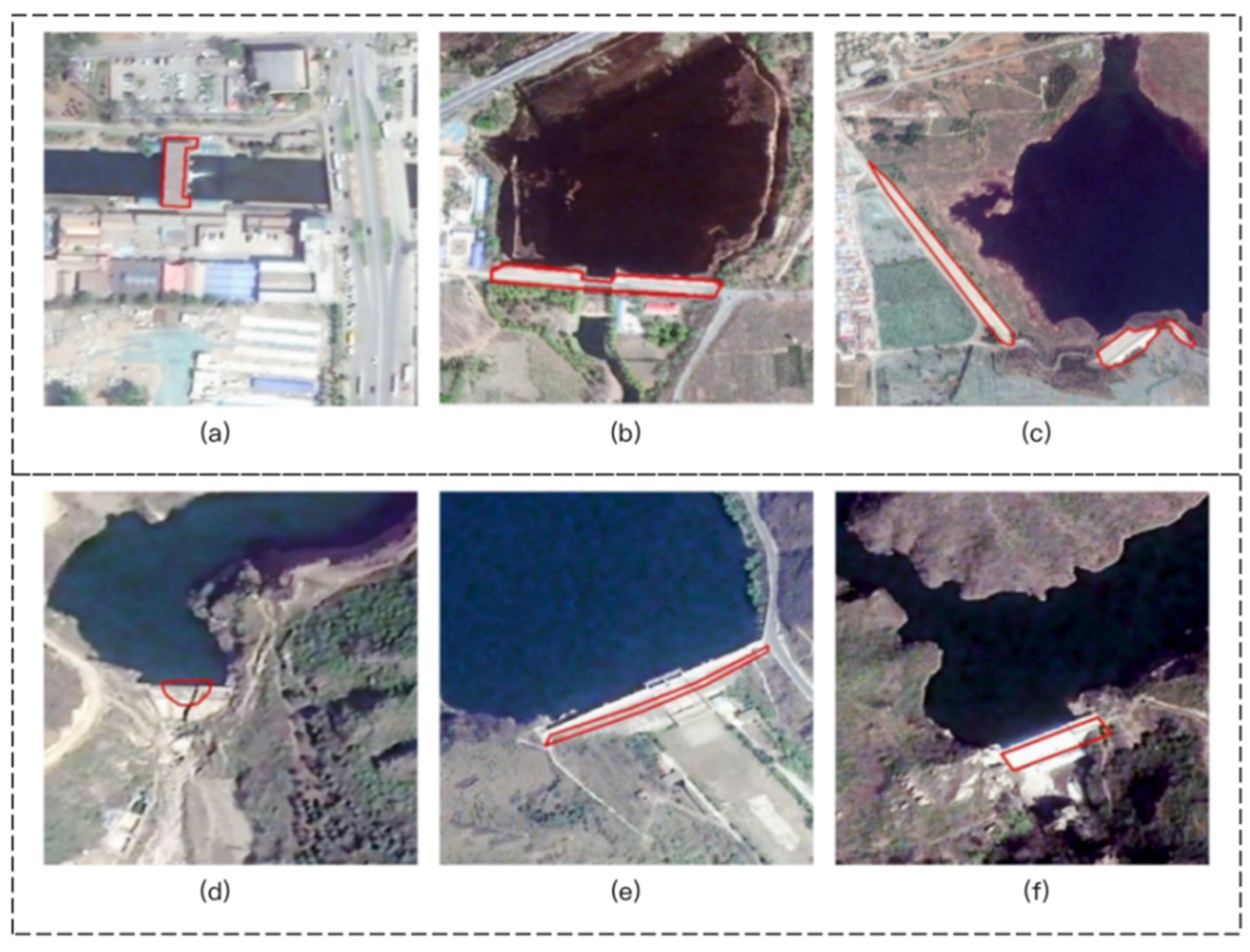
Remotesensing 14 04049 g019
Figure 20. Examples of OSM Dams overlapped by satellite images. (ac) Well-matched dam masks; (df) poorly matched dam masks.
Remotesensing 14 04049 g020
Table 1. The allocation of samples in RSDams for training, validation, and testing.
DatasetCategoriesTrainingValidationTestTotal
RSDamsImage patches12803204002000
Dam13303264162072
Table 2. Comparison of the structures of YOLOv5s and YOLOv5s-ViT-BiFPN.
YOLOv5sYOLOv5s-ViT-BiFPN
InputImages or PatchesImages or Patches
BackboneCSPDarknet53
(Focus, CSP, CBL, SPP)
CSPDarknet53
(Focus, CSP, CBL, SPP), ViT
NeckPANetBiFPN network
Head/PredictionYOLOv3 headYOLOv3 head
Table 3. Comparisons of accuracy and time for training with different detection models and training methods on the RSDams validation set.
Training MethodModelnAccuracy (%)Training Time (h)
PrecisionRecallF1mAP
Learning from ScratchSSD----80.11.3
YOLOv3-78.477.978.171.39.3
YOLOv5s-81.278.779.976.64.2
YOLOv5s-BiFPN-83.281.682.478.54.3
YOLOv5s-ViT-BiFPN-84.882.783.780.24.4
Transfer Learning with Different Frozen LayersYOLOv5s-ViT-BiFPN083.28081.673.13.1
185.382.88479.21.0
284.984.184.580.11.0
388.285.386.781.81.0
487.882.585.179.31.0
587.783.885.780.10.9
687.181.284.178.80.9
786.179.482.677.30.9
884.780.682.676.50.9
983.177.880.470.40.9
Table 4. Comparison of generalization errors on the RSDams and DIOR Dams test sets.
ModelNMSRSDams Test SetsDIOR Dams Test Sets
Omission Errors (%)Commission Errors (%)Omission Errors (%)Commission Errors (%)
SSD-8.45.020.11.7
YOLOv3-10.15.318.72.7
YOLOv5s-ViT-BiFPNNMS3.612.616.38.4
Adaptive-SDT-NMS3.64.116.30
Table 5. Evaluation results of dam detection in two study areas. (A check mark means the method is used.)
Study AreaJCR-GSWESANumbers of Predicted Bounding BoxesTrue PositivesFalse NegativesPrecision (%)Recall (%)
Yangbi 1051039.576.9
489418.869.2
8310310.876.9
449420.569.2
Changping 17082341.485.2
6502253.981.5
14712251.581.5
6202253.681.5
Table 6. Accuracy comparison of dam segmentation results with and without the SLIC algorithm. (A check mark means the method is used.)
SLIC AlgorithmAverage Overall Accuracy
(%)
Average Kappa (%)Average Omission Errors (%)Average Commission Errors (%)
97.50.460.244.7
97.40.77.144.3
Table 7. Comparison of the number of dams in Yangbi and Changping from different datasets with visual interpretation results.
DatasetData FormatNumber of Dams in YangbiNumber of Dams in Changping
Visual Interpretation ResultsGeographical Point1327
Our MethodDam Masks Raster922
GOODDGeographical Point42
GRanDGeographical Point00
OSM DamsDam Polygon Vector211
Publisher’s Note: MDPI stays neutral with regard to jurisdictional claims in published maps and institutional affiliations.

