Modelling the Influence of Geological Structures in Paleo Rock Avalanche Failures Using Field and Remote Sensing Data

Abstract

This paper focuses on the back analysis of an ancient, catastrophic rock avalanche located in the small city of Lettopalena (Chieti, Italy). The integrated use of various investigation methods was employed for landslide analysis, including the use of traditional manual surveys and remote sensing (RS) mapping for the identification of geological structures. The outputs of the manual and RS surveys were then utilised to numerically model the landslide using a 2D distinct element method. A series of numerical simulations were undertaken to perform a sensitivity analysis to investigate the uncertainty of discontinuity properties on the slope stability analysis and provide further insight into the landslide failure mechanism. Both numerical modelling and field investigations indicate that the landslide was controlled by translational sliding along a folded bedding plane, with toe removal because of river erosion. This generated daylighting of the bedding plane, creating kinematic freedom for the landslide. The formation of lateral and rear release surfaces was influenced by the orientation of the discrete fracture network. Due to the presence of an anticline, the landslide region was constrained in the middle-lower section of the slope, where the higher inclination of the bedding plane was detected. The landslide is characterized by a step-path slip surface at the toe of the slope, which was observed both in the modelling and the field. This paper highlights the combined use of a geological model and numerical modelling to provide an improved understanding of the origin and development of rock avalanches under the influence of river erosion, anticline structures, and related faults and fractures.

1. Introduction

Catastrophic rock avalanches can involve rock failures of million cubic meters in size [1,2,3] that lead to high velocity flows of fragmented rocks with the release of enormous energy that can be highly destructive [4,5,6]. In addition, rock avalanches may cause indirect hazards related to their debris flow deposition (e.g., upstream flooding induced by river obstruction) [7,8]. Unfavourably oriented discontinuities are deemed to be one of the critical preconditioning factors for rock avalanches [9,10,11,12,13]. It has been found that catastrophic rock avalanches are usually related to the presence of large and persistent discontinuities (e.g., faults and bedding), which is emphasized by the cases of translational sliding [14,15], wedge sliding [16], and toppling failures [17]. The influence of the local fracture network has also been observed in catastrophic landslides, contributing to the disintegration of the failed rock mass and the formation of release surfaces [18,19].

For rock landslide analysis, the interpretation of on-site discontinuity orientation and persistence is critical as it can provide the basis for rock mass characterization, estimation of rock mass properties, and the prediction of possible failure mechanisms [20]. Discontinuity characterisation has been conventionally performed through traditional manual surveys used to collect important information on discontinuity geometry, orientation, and strength properties [21]. However, engineering-geology survey use is limited to hazardous or inaccessible sites (e.g., coastal cliffs, unstable slopes, and steep slopes). Recent advancements in remote sensing (RS) techniques can provide a 3D topographic mapping of outcrops at these sites, thus allowing remote discontinuity detection. These include the utilization of aerial/terrestrial light detection and ranging (LiDAR) mapping to directly acquire a 3D point cloud (or TIN mesh) of an outcropping rock mass [22]. Digital photogrammetry can also be deployed to acquire a series of stereo images to construct 3D topography of outcrops by using a structure-from-motion (SfM) algorithm [23,24]. The application of optical sensors mounted on unmanned aerial vehicles (UAV) for digital photogrammetry, termed UAV remote sensing (UAV-RS), becomes a low-cost, lightweight, time-saving, and user-friendly option to map rocky outcrops where discontinuities daylight [23].

Following the interpretation of on-site discontinuities, stability analysis can then be undertaken. Initial evaluation of potential instability is typically undertaken through kinematic analysis to predict potential failure modes of discontinuous rock slopes. The inclusion of internal (weight) and/or external stresses (e.g., pore-water pressure, earthquake loading, and the effect blasting) can be undertaken using 2D and/or 3D limit equilibrium (LE) analysis to evaluate the factor of safety (FoS) of a rock block that is constrained by a simple geometrical representation of the identified discontinuities [25]. Both kinematic and LE analysis can provide an initial estimation of the stability condition of a rock slope. However, they are not applicable for the analysis of slope displacement and other complex situations, e.g., anisotropic and/or heterogeneous rocks and complicated discontinuity networks [26]. Numerical modelling, especially based on discontinuum and hybrid methods, can provide further insight into landslide failure mechanisms, particularly where the discrete fracture network has a controlling influence on potential failure [27]. For example, discontinuum modelling has been preferentially employed to investigate the displacement and/or deformation of rock blocks [28] and used for the analysis of rockfalls and the mobility or run-out of landslides as large displacements and rotation of blocks are allowed in the modelling [29,30].

Therefore, it is clear that rock mass characterization plays a key role in the analysis of rock failures. Another crucial aspect in such types of analyses is represented by the geological and evolutional model of the area. During the numerical simulation, the structural and geological models are often simplified to facilitate the modelling process. However, the structural/geological model can play a key role in understanding the evolution of the rock avalanche failure mechanism [9,31].

In this context, this paper presents the representative case study of the Lettopalena rock avalanche to examine the influence of an anticline on a catastrophic translational landslide in sedimentary rocks. The Lettopalena rock avalanche occurred at approximately 4.8 kyr BP [32], and it is in the Italian Apennines, where the influence of structural/tectonic features plays a key role in the evolution/triggering of such large phenomena. The rock avalanche, the estimated volume of which was around 30 × 10⁶ m³ [33], has been studied over the years by several authors who have analysed both the ancient rock avalanche mechanisms and evolution [32,34] and the most recent rockfall events. In fact, several rockfalls event have been documented in recent decades [35], with the most recent one dated 2005 and estimated at around 2000 m³ by Bianchi-Fasani et al. [33]. Such rockfall events are mainly controlled by the unfavourable orientation of structural features (bedding and joints) and by water infiltration along discontinuities [33]. Such minor events must be studied in a more general context that involves the structural-morphotectonic evolution of the area, which has led to failures varying from a few cubic meters to millions of cubic meters (such as the Lettopale rock avalanche [32,34].

Scarascia-Mugnozza et al. [32] performed a comprehensive study of morphological, structural, and lithological constraints on the rock avalanche slope. A geological and numerical model of the rupture developed by the authors highlighted the key role of the pre-existing topography/geomorphic features and the high deformability of the out-cropping Mio-Pliocene formation.

Most recently, further studies in the area have been carried out by Bianchi Fasani et al. [34], who developed a morpho-structural evolution model of the study area by the integration of detailed geological–structural and geomorphological surveys. Based on this model, the authors performed numerical simulations through the Finite Difference Method (FEM) with the goal of evaluating the effect of the uplift-related morphological changes of the valley–slope system and the role of the horizontal/vertical stress ratio variations due to geodynamic regime shifts. The results of the modelling presented by the authors confirmed the presence of stress–strain conditions associated with the massive rock slope failures which occurred.

In this context, this research aims to integrate the existing studies with a different type of numerical simulation/model, carried out using the discrete element method, to highlight the role of the structural setting (bedding inclination) and potential river erosion in the Lettopalena rock avalanche. Various RS techniques (i.e., UAV-RS and satellite RS) have been combined to detect structural features and post-landslide features. Subsequent 2D modelling was employed to simulate, as mentioned above, the development of the landslide following river erosion at the toe of the slope. The remotely captured data was used to constrain and validate the numerical modelling undertaken. It will be highlighted how the geological model and the interpretation of the geological-geostructural evolution of the area can play a key role in the results of rock avalanche numerical back analyses. The use of distinct element analysis, combined with previous FEM simulation [32,34], can represent a further tool for landslide interpretation.

2. Study Area Description

The study area is located in the Central Apennines of Italy, at 40°00′35″N 14°09′56″E, on the NW side of Lettopalena in Chieti, at an altitude in the range of approximately 500 m a.s.l. to 1200 m a.s.l. (Figure 1). The valley where the rock avalanche is sited is the Caramanico Valley, a north–south-oriented tectonic depression located on the SE of Monte Amaro and about 40 km west of the Adriatic Sea. The area is still monitored for potential instability due to the hazard posed to a village built up adjacent to landslide deposits and the section of a state road (SS84) constructed along the landslide scar. A recent landslide, which occurred on the 20 April 2005 that resulted in a 2000 m³ rock block failure, highlights the ongoing risk. The run-out from the failure blocked the SS84 state road, destroyed a private house along the route, and led to the death of one resident.

2.1. Geological Setting

Geologically, the study area is situated on the southeast side of the Majella anticline on a carbonate platform succession [36]. The platform is characterized by an N–S oriented anticline with a steeply-dipping forelimb and a thrust fault underlying the Majella unit at the E margin [36,37]. The sedimentary record of the platform comprises a wide time interval from the Late Jurassic to the late Miocene [36]. The undeformed platform was initially formed, transecting approximately 20 km long to the adjacent northern basin, which was separated by a 1000-m-high non-depositional escarpment trending E-W [36]. During the Cretaceous period, basinal sedimentary rocks buried the escarpment, causing the gradual decrease of the slope angle [36]. At the end of the Campanian, the basin was almost filled, and the Maastrichtian sequences were deposited onto the platform, consequently forming a distally steepened ramp [36,38,39]. A carbonate ramp, consisting of Bolognano formation, was subsequently developed overlying the shallow water deposits during the late Rupelian to early Messinian interval [38]. The schematic platform-basin cross section has been provided by [36].

On a local scale, a primary geological characteristic is the Molise unit overlying the younger Majella unit, which was caused by overthrust faulting. The major component of the Molise unit is the Argille Policrome (APO), comprised of the alternation of pinkish/reddish to greenish marly claystone, chert, and calcilutite. The Majella unit, in the order of the depositional sequence from the bottom to top, is composed of Morrone di Pacentro Formation (MOR), Monte Acquaviva Formation (ACQ), Scaglia Formation (SCZ), Orfento Formation (OR), Santo Spirito Formation (FFS), Bolognano Formation (BOL), Gessoso-Solfifera Formation (GES), and Majella Flysch (MAJ) [40]. The characteristics of these formations are summarized in

Table 1. Characteristics of the formations that constitute the Majella unit [40].

Formation		Lithology	Thickness
MAJ		Yellowish pelite with decimetres-to-metres thick intercalations of sandstone	˃900 m
GES		Gypsum and gypsumarenite deposits intercalated in alternating grayish marl and siltstone	30–100 m
BOL	BOL1	Marly limestone and cherty limestone	0–20 m
	BOL2	Bryozoan-rich calcarenite	0–70 m
	BOL3	Massive-bedded whitish limestone with rodolites of coralline algae, bryozoan, echinoids, molluscs, macroforaminifera	30–60 m
FSS	FSS1	Whitish calcilutite with chert alternating with calciturbidites	20–50 m
	FSS2	Whitish-to yellowish porous calcarenite with chert	100–300 m
OR		Biocalcarenite and whitish porous calcirudite	60–200 m
SCZ		White hemipelagic calcilutite, in decimetres thick beds, with red-to violet chert, alternating with porous bioclastic calcisiltite and calcarenite	50–400 m
ACQ		White fine-grained biocalcarenite and calcirudite rich in Rudists	200–300 m
MOR		Massive micritic limestone and oolitic and oncolitic calcarenite	˃400 m

. In addition, Talus Deposits are distributed in the valleys adjacent to the analysed slope, consisting of well-sorted centimetres-to-decimetres sized rock fragments that are characterized by openwork to partially openwork texture [40]. Figure 2a shows the geological map of the area after Vezzani and Ghisetti [41] and Miccadei et al. [42]. The base Digital Elevation Model (DEM) used in the map is the 10 × 10 m resolution DEM available from Abruzzo Region GIS portal (http://geoportale.regione.abruzzo.it/Cartanet, accessed on 1 May 2019). The slope profiles 1–4 in the geological map have been created to highlight landslide geometry. Profile 2 has been used to create the 2D geological section of Figure 2b. Profiles 1, 3, and 4 will be shown and discussed in Section 4.1.

Regarding the structural geology, the slope is characterized by the convex relief of the bedding as the presence of an anticline, whose bedding inclination undergoes a gradual increase from sub-horizontal angles (10°–20°) on the crest of the slope to tilted angles (25°–30°) in the medium-low part of the slope (Figure 2). There are two thrust faults in the analysed slope (Figure 2a). One is dipping towards SE and causing the Molise unit to overlie the Majella unit (as aforementioned), and the second dipping towards NW and resulting in uplift of hanging wall of Majella unit.

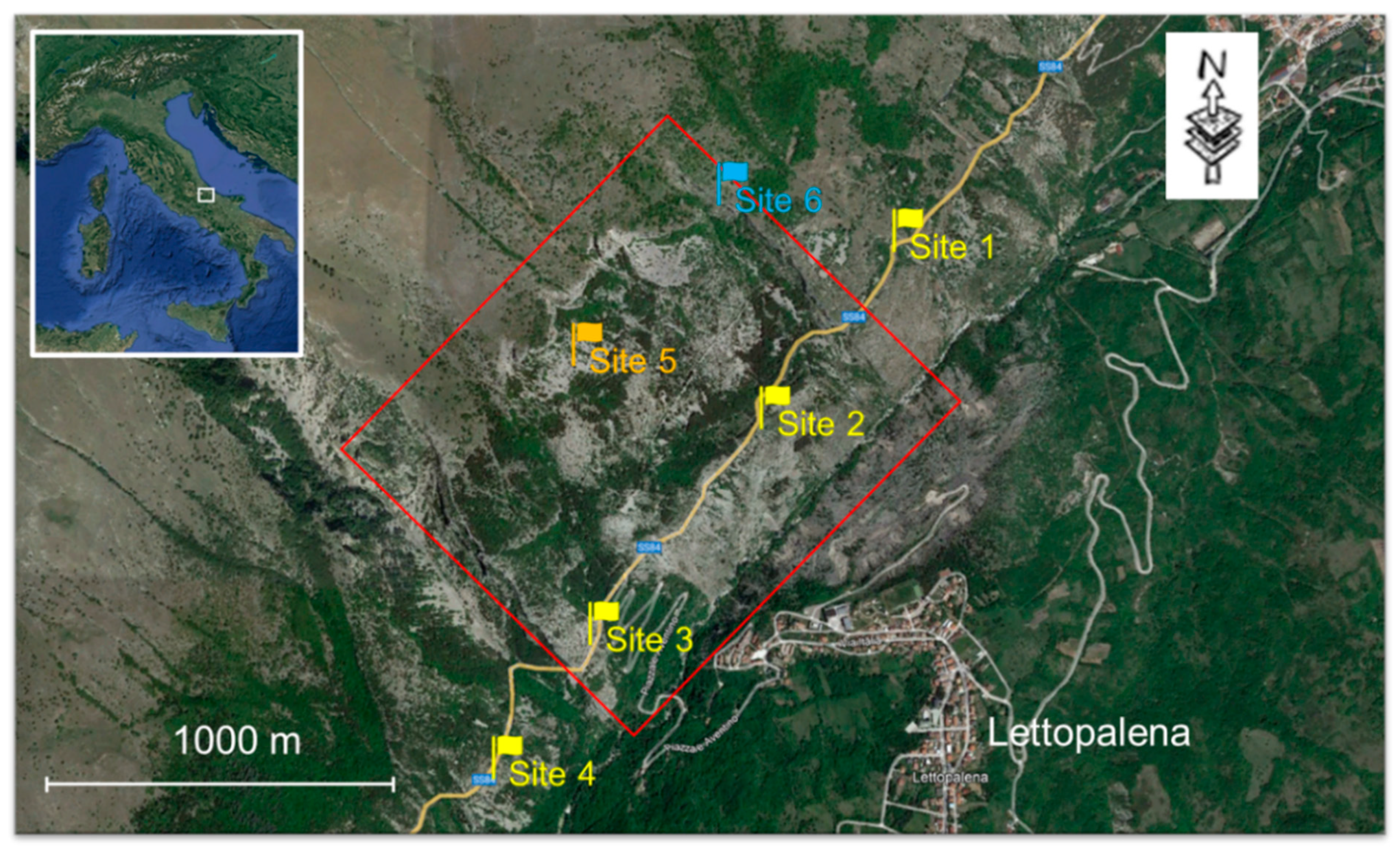
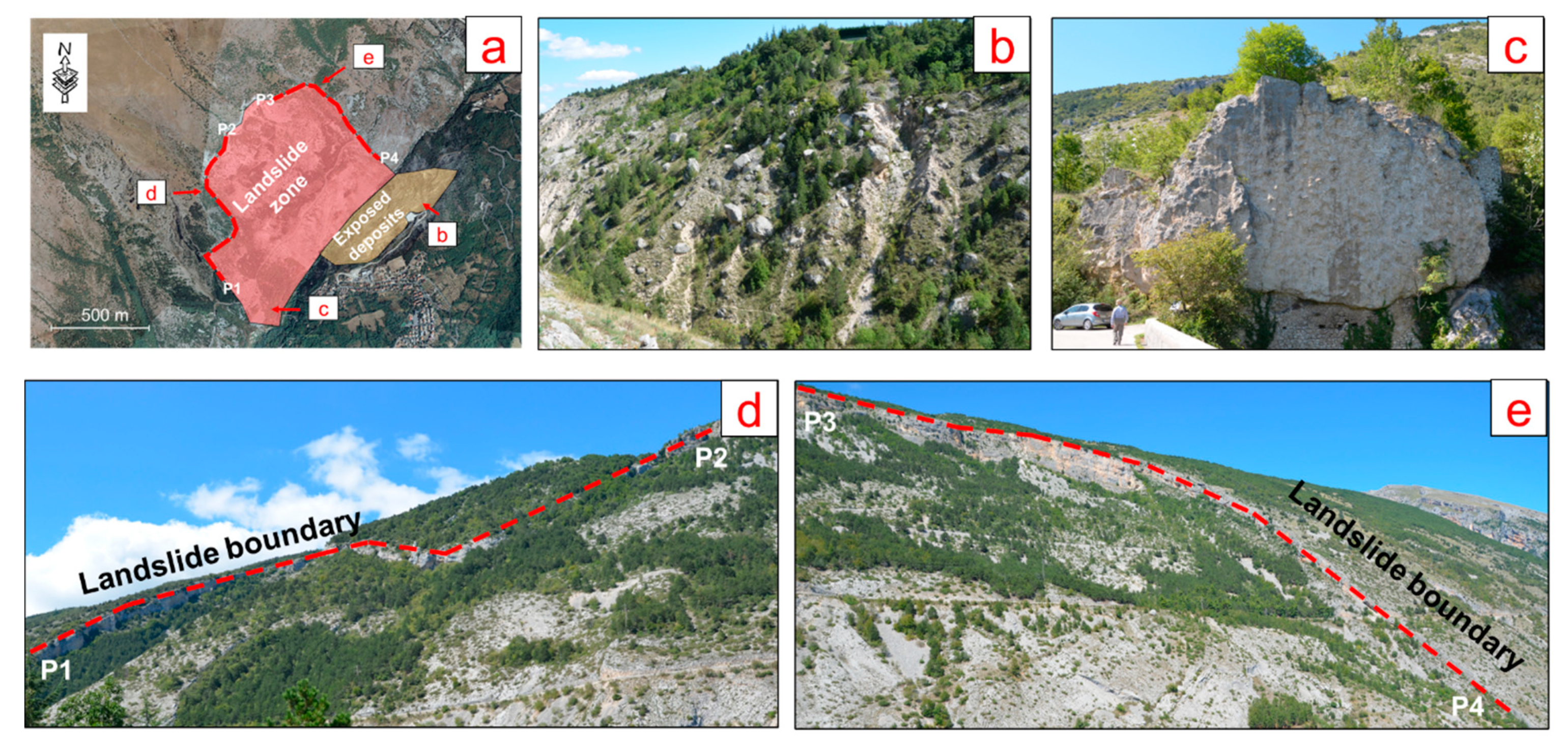
2.2. The Lettopalena Paleolandslide

The Lettopalena Paleolandslide (sometimes named Taranta-Peligna Paleolandslide) is a historic landslide with a delineated boundary (shown in Figure 3a) that probably occurred in the Mid- Holocene [35]. The landslide features an elongated headscarp characterised by a ‘Z’ shape on the SW side (Figure 3d) and a right-angle corner on the NE side (Figure 3e). Landslide deposits, composed of scree and talus with various sizes of fragmented rocks (Figure 3b), are observed at the toe of the slope and on the opposite side of the valley where the village of Lettopalena has been built. Some blocks, tens of metres in size, are still visible at the toe slope and along the river, which testify to the heterogeneity of the paleo-landslide deposits. An example of such blocks is shown in Figure 3c; the planar condition of the block surface facing the camera implies the block was detached along a highly persistent geological structure.

Although there is a scarcity of additional detail for the ancient landslide, a recent small-scale landslide in 2005 [33], adjacent to the study site, can be a useful indicator of potential triggers for the ancient landslide. The two landslides are located in identical geological environments and have a similar mechanism that is controlled by the bedding and the lateral and rear release surfaces and were defined by the discrete fracture network. For the 2005 landslide, rainfall was suggested as a contributing trigger factor [33]. This may also be applicable to the catastrophic landslide because water saturation is effective in reducing the shear strength of discontinuities [43,44]. Paolucci et al. also suggested that the paleolandslide may have been triggered by an earthquake [35], as for other paleolandslide in the region (e.g., Scanno Paleolandslide, [31]). The high mobility of the landslide is evidenced by the distribution of landslide deposits in proximity to the village (see Figure 3a,b), with the presence of talus deposits on the opposite flank of the valley that ran out 150 m away from the toe of the slope.

3. Materials and Methods

3.1. Interpretation of Geological Structures and Kinematic Analysis

Geological structures were interpreted through the combination of traditional manual surveys and RS mapping to investigate the potential mechanism and kinematics of the landslide. More precisely, in relation to the six survey sites shown in Figure 1 (sites 1–6), traditional manual surveys and terrestrial photogrammetry have been carried out at accessible sites (sites 1-2-3-4 of Figure 1) between 2019 and 2021. Sites 5 and 6 were investigated using Google Earth satellite imagery from 2009 (site 5) and a UAV survey (site 6). This provided a method to gather further structural information in the inaccessible upper part of the landslide scar and therefore verify that main lineaments have a constant orientation along the entire slope.

At sites 1–4, a scanline survey was conducted at each location to detect on-site discontinuities with the measurement of their properties, including orientations (dip and dip direction), estimated joint wall compressive strength (JCS), spacing, persistence, surface weathering condition, surface shape and joint roughness coefficient (JRC). Persistence is measured by the exposed trace length of a discontinuity.

Additional discontinuity data were collected at sites 1-2-3-4 through terrestrial photogrammetric mapping to complement and verify the results of manual surveys. Terrestrial photogrammetry provides a series of stereo images to construct a 3D point of rock outcrops by using the SfM technique, which was carried out by using the Agisoft Metashape software [45]. Based on the point cloud, local geological structures (joints and fractures) were manually identified by using the Compass plugin [46], provided by CloudCompare software [47]. The plane tool of the Compass plugin was used to measure the orientation of an exposed planar structure where its plane was fitted to all points sitting within the circle (using least squares). This method provides an orientation estimate (dip/dip direction) for the fitted plane. The use of this software made it possible to plot the data on a stereonet for comparison with the conventional engineering geology data.

A 2019 satellite image at site 5 (Figure 1) was obtained from Google Earth, orientated towards the north. Using this image, it was possible to determine the strike of daylighting discontinuities.

Site 6 is a representative section of the landslide scarp at the upper right corner of the failure zone. This area was surveyed using UAV photogrammetric mapping in October 2019. A total of 92 photographs were acquired with a lateral and vertical overlap of 70/80%. The aircraft used for the survey was a DJI Mavic 2 Pro, and the final resolution of the extracted point cloud was between 3 and 4 cm.

An analysis was undertaken to evaluate the kinematic potential of the slope (dip/dip direction: 40°/110°) for planar sliding, wedge sliding, and direct toppling using the features and discontinuities identified at the six sites described above.

Finally, satellite DEM data (10 × 10 m resolution, provided by Abruzzo Region) was used to identify the post-landslide features for the entire slope. Various thematic maps have been generated using the lidar data, including a slope map to delineate the inclination of the slope, a hillshape map to produce a grayscale 3D representation of the terrain surface, and an aspect map to quantify the slope direction. A 2022 Google Earth image (0.5 × 0.5 m) was used to interpret the geometric characteristics of the failure scar at the toe of the slope.

3.2. Numerical Analysis of the Landslide and Sensitivity Study

Given the landslide characteristics (i.e., a structurally-controlled mechanism and relatively simple geometry), the 2D Universal Distinct Element Code (UDEC) [48] was used to model the landslide. The code uses an explicit time-stepping system to solve equations of motion, simulating the response of rock mass that is subject to either static or dynamic loading. In the model, a rock slope is represented as an assemblage of discrete blocks separated by discontinuities which are treated as boundary conditions between blocks. In this case study, individual blocks behave as deformable, and deformation behaviours are defined by the Mohr-Coulomb failure criterion. Typical limestone property values, as provided in

Table 2. Rock properties associated with Mohr-Coulomb failure criterion [49].

Density	Shear Modulus	Bulk Modulus	Friction Angle	Cohesion	Tensile Strength
2750 kg/m3	30 GPa	50 GPa	40°	8 MPa	2.5 MPa

, were used for landslide modelling [49].

3.2.1. Landslide Back Numerical Analysis

Using the geological section in Figure 2 and post-landslide slope geometry that was delineated using satellite DEM data (10 × 10 m resolution, provided by Abruzzo Region), pre-landslide scenarios have been constructed along profile 2 (Figure 4). The models highlight how the thrust fault at the toe of the slope generates the contact between the BOL and the GES formations. The BOL formation, being made of limestone materials, has higher erosion resistance compared with the GES formation. Therefore, we have indicated that the Aventino River erodes the GES formation at the toe of the slope, daylighting the bedding planes of the BOL formation. The erosional evolution (pre-failure) has been illustrated in Figure 4a. Figure 4b shows the current slope profile (post-failure) with landslide deposits at the toe of the slope and on the opposite side of the valley.

Using the assumed pre-landslide slope geometry (as shown in Figure 4a), the 2D distinct element model in UDEC (Figure 5) was created. The model incorporates the identified discontinuity network (i.e., S0 and J1) with the properties listed in

Table 3. The property of discontinuities used in numerical modelling.

Normal Stiffness	Shear Stiffness	Friction Angle	Cohesion
10 (GPa/m)	5 (GPa/m)	22 (°)	25 (KPa)

, but with sets J2 and J3 excluded from the modelling as they are sub-parallel to the cross-section. Generic properties of discontinuity and rock were used for numerical modelling. The values of these parameters were determined within reference to relevant literature [50] and calibrated through back analysis. The thrust fault is considered with the uplift of the hanging wall in which a folded bedding plane is configured by a curve of 20° inclination at the crest of the slope and 25° inclination at the toe of the slope.

Gradual river erosion is also incorporated into the modelling through the sequential removal of rock blocks in three stages. Note that the folded bedding plane at the base of the modelled slope does not daylight until the third stage of erosion is completed. The modelling sequence occurred between 2021 and 2022 and consisted of 4 simulation intervals (1–4). Interval 1 simulates the mechanical behaviour of the slope before river erosion); Interval 2 models the mechanical behaviour of the slope in response to stage 1 of the simulated river erosion; Interval 3 is associated with the mechanical behaviour of the slope in response to stage 2 of the simulated river erosion; Interval 4 models the mechanical behaviour of the slope in response to stage 3 of the simulated river erosion.

A fixed boundary condition was applied to the sidewalls and the base of the model. Boundaries (sidewalls and the base) were extended 200 m from the zone of interest to ensure no boundary effects on the zone of interest. Three representative history points (H1, H2, and H3) were placed in BOL rocks within the model to monitor the displacement of BOL in the lower, middle, and upper parts (see Figure 5) of the modelled slope.

3.2.2. Sensitivity Analysis

In numerical simulations, material properties are usually the most difficult parameters to determine. In this context, a sensitivity analysis was carried out to assess the potential impact of variations in the material properties on the modelling of the landslide. Considering that the catastrophic landslide was most likely associated with translational sliding along bedding planes, the sensitivity analysis focused on the variation of the friction angle and cohesion of S0, as shown in

Table 4. Variations in dip, dip direction, persistence, friction angle of the folded bedding plane were characterized by mean, minimum and maximum values.

J1 Property	Mean Value	Minimum	Maximum
Friction angle (°)	22	17	27
Cohesion (Pa)	2.5 × 104	0	5 × 104

. For each parameter, a sensitivity analysis was performed by varying its value from the minimum, the mean, to the maximum using a control variate method [28] in order to examine the influence of the uncertainties on the slope stability analysis.

4. Results

4.1. The Characteristics of Geological Structures and Result of Kinematic Analysis

4.1.1. The Characteristics of Geological Structures

As discussed in Section 3, the characteristics of the geological structures have been investigated through different survey methods. Traditional manual surveys and terrestrial photogrammetry have been performed at sites 1-2-3-4. A total of 79 discontinuities were measured using the traditional manual approach and a further 81 through photogrammetric analysis. Figure 6a shows a lower hemisphere stereonet plot representing the poles of 76 discontinuities (joints and bedding planes) collected from traditional manual surveys at sites 1-2-3-4, where four main discontinuity sets (S0, J1, J2, and J3) were identified. Figure 6b presents a stereonet representation of the poles of 81 discontinuities measured from the terrestrial and UAV photogrammetric surveys at sites 1-2-3-4-6. Both results are generally consistent, although J3 is less pronounced.

The two datasets were then combined (Figure 6c). The relatively low-angle discontinuities dipping towards SE in set S0 are related to the bedding of Majella rock units, with a mean orientation (35°/099°) and high persistence (more than 20 m); J2 (81°/257°) and J3 (80°/230°) are sub-parallel with J2 being the predominant one; joints in sets J1 (80°/348°) and J2 are sub-vertical and sub-orthogonal to each other. J1, J2, and J3 are less persistent compared with S0, whilst they have similar degrees of spacing (approximately 0.4 m) throughout the four sampling sites (

Table 5. Properties of identified discontinuity sets, including the mean orientations obtained from the traditional manual survey, mean orientations obtained from photogrammetric surveys, mean orientations obtained from the combination of both surveys, mean discontinuity spacing and mean discontinuity persistence.

Set	Mean Orientation (Dip°/Dip Direction°)			Mean Spacing (m)	Mean Persistence (m)	Mean Infilling (mm)
	From Traditional Manual Survey	From 3D Model	Combined
S0	36/105	33/93	35/99	0.4	>20	Hard filling < 5
J1	84/341	74/356	80/348	0.3	1–3	Hard filling < 5
J2	83/257	78/255	81/257	0.4	1–3	Hard filling < 5
J3	80/230	(Nah)	80/230	0.4	1–3	Hard filling < 5

). The spatial relationship between S0, J1, and J2 and their geometric characteristics are presented in Figure 7, which shows a terrestrial photogrammetric built 3D model for a roadside section of the analysed slope.

Table 6. Site-dependent discontinuity properties (site 1/site 2/site 3/site 4), including UCS, surface weathering condition, surface shape and JRC.

Set	JCS (MPa)	Weathering	JRC
S0	50/32/48/44	moderately/slightly/moderately/moderately	3/7/3/1
J1	44/30/50/48	moderately/slightly/moderately/moderately	3/7/3/3
J2	50/30/44/50	moderately/slightly/moderately/moderately	3/9/5/3
J3	48/30/(Nah)/50	moderately/slightly/(Nah)/moderately	3/9/(Nah)/3

summarizes geomechanical discontinuity properties (i.e., JCS, weathering condition, surface shape condition and JRC) at sites 1-2-3-4 (where traditional manual survey was conducted). Discontinuity properties measured at site 2 differ from the properties detected at other sites. For example, for the four sets, the JCS measured at site 2 is lower than the one measured at sites 1, 3, and 4. Less weathering and increased undulation of discontinuity surfaces was observed at site 2.

Regarding sites 5 and 6, as mentioned in Section 3, they have been investigated using Google Earth satellite images (site 5) and a UAV survey (site 6). This provided a basis to validate the results gathered from the traditional manual surveys and terrestrial photogrammetry and, more importantly, to confirm that the orientation of major lineaments at the crest of the landslide scarp was similar to the ones measured along the state road (SS84). Figure 8a shows the strikes of daylighting discontinuities on a Google Earth at site 5, where the observed discontinuities are delineated by blue and red lines. From the rosette plot of strikes of the features (Figure 8b), the discontinuities highlighted in blue are SSW-NNE trending, and discontinuities highlighted in red are SSE-NNW trending, implying their close relation with J1 and J2/J3, respectively (Figure 6). However, discontinuities related to S0 are absent in the image as S0 is parallel to the slope surface and has less potential for daylighting on the slope.

The UAV photogrammetry at site 6, with a flight plan depicted in Figure 9a, generated a 3D point cloud consisting of approximately 36 million points with spatial resolution between 3 and 4 cm to delineate the section of the escarpment. Where X indicates the E direction, Y points towards the N direction, and Z infers the vertical (Figure 9b). The survey was unable to map the entire base of the valley due to occlusion caused by vegetation. However, two sections of the escarpment related to the rear and lateral release surfaces of the landslide are clearly presented. It shows that two sections of the escarpment are characterized by near-vertical limestone cliffs of 60-m height. The rear release surface is formed by major features (88°/155°) belonging to J1, while the lateral release surface by two features (79°/202° and 85°/038°) belonging to J2/J3. The bare slope (slip surface) underlying the escarpment also exhibits a low-angle planar surface related to bedding.

Regarding the 10 × 10 DEM analysis, the raster data presents a clear topographic contrast between the carbonate reliefs of the NW slope, with altitudes exceeding 1700 m a.s.l., and the predominantly clayey hilly landscape of the SE foothills, with average altitudes of less than 900 m a.s.l. (Figure 10a). The contact between the two parts is marked by the deep incision of the NE-SW trending Aventino river valley (Figure 10b). The SE slope underlying the Lettopalena village exhibits a flat terrain represented by low slope angles in Figure 10c and white colour on the hillshade map (Figure 10d). Compared with the SE slope, the NW slope is relatively steep, characterized by a convex terrain where the inclination, in general, increases from the crest to the toe (Figure 10c). In addition, the slope where the landslide occurred is constrained by two valleys (the NE-SW trending Aventino river valley and an NW-SE trending valley).

The landslide scar is also clearly visible on these maps. For example, the elevation map (Figure 10a) and the hillshade map (Figure 10d) identify the landslide zone through a sudden colour change. The high slope angle values (approximately 70°) highlighted in red along the upper landslide boundary indicate the presence of an escarpment connecting the NW-SE trending valley at the lower sector of the slope (as shown in Figure 10c).

The landslide extent is depicted in the high-resolution satellite image (Figure 3a) and the thematic maps (Figure 10) with a measured area of 0.94 million m². In addition, the thickness of the BOL rock layer (failure body) is approximately 50 m according to the height of the escarpment (Figure 9b). It is estimated that the failure volume of the catastrophic landslide was approximately 4.7 million m³.

Using the DEM data, 2D geometric models have been generated along the four slope profiles of Figure 2a to highlight the terrain change associated with the landslide (Figure 11). Profile 1 is out of the landslide zone, while profiles 2–4 pass across the landslide zone and capture the geometry of the landslide scar. It can also be seen in profiles 2–4 that the upper boundary of the landslide is marked by the presence of an escarpment and located at approximately 1000 m a.s.l. In addition, the height of the escarpment gradually reduces from profile 2 to profile 4 (from NE to SW).

4.1.2. Results of Kinematic Analysis

The kinematic analysis highlighted that the slope is prone to planar sliding along a subset of the set S0/bedding (Figure 12a). Wedge sliding is also possible, constrained by S0/J1 and S0/J2 and slides along S0 (Figure 12b). Concerning potential direct toppling, J1 and J2 could intersect to form block edges dipping into the slope, and S0 acts as the potential basal sliding surface (Figure 12c). The results of kinematic analysis highlight the dominant influence of bedding (set S0) on the potential for planar sliding, wedge sliding, and direct toppling.

The topographic mapping highlights that the slope exhibits a convex terrain, with an increasing slope angle towards the toe (Figure 10c). Furthermore, at the toe of the slope during the phases of river erosion, the slope face alongside the river could reach an inclination much higher than 20–25°. In this context, the kinematic analysis examined the kinematic potential of the slope for planar sliding with different values of slope angle (

Table 7. Probability of planar sliding along S0 with different slope angles.

Slope Angle	40°	50°	60°
Probability for all joints	10.19%	14.01%	14.01%
Probability for S0	59.26%	81.48%	81.48%

). When the slope angle is 40°, 59% of joints in S0 can behave as a slip surface for potential planar sliding. This percentage was calculated based on the total number of the surveyed planes of S0. Increasing the slope angle allows a higher probability of planar sliding. When the slope angle increases above 50°, the probability of failure achieves a convergence.

4.2. Landslide Numerical Modelling and Sensitivity Analysis

4.2.1. Landslide Numerical Modelling

Figure 13 shows a modelling result associated with slope displacement in the X direction after river erosion. The modelling successfully simulates the catastrophic translational sliding along the bedding plane. The result supports field observations and the depicted evolution of the area (Figure 11), with the lower and middle sections of the slope being susceptible to failure. The landslide is characterized by a step-path slip surface at the toe of the slope, as highlighted in the close-up image 2 in Figure 13. At the NW tip, the failure terminates in the upper-middle section of the slope, and the headscarp is defined by the interaction and connection of S0 and J1, as highlighted in the close-up image 1 in Figure 13.

The X displacement of the history points has been recorded with the advancement of the modelling sequence (Figure 14). The modelled sequence consists of 4 temporal intervals of calculation timesteps.

(1)

Interval 1 (timestep 0–100,000): The three history points all achieve a limited equilibrium state that is characterized by the convergence of X displacement. During this interval, H3 experiences more X displacement than H2/H1.

(2)

Interval 2 (timestep 100,000–180,000): During this interval, H1/H2/H3 are stable and experienced a minor increase in X displacement, caused by the debuttressing induced by river erosion. This debuttressing provides a gradually attenuated impact on the slope from H1 to H3, showing that H1 increased X displacement to 0.3 mm.

(3)

Interval 3 (timestep 180,000–260,000): Similar to interval 2, H1/H2/H3 remain stable. Additional increases in X displacement of the three history points can be observed. During interval 3, the debuttressing effect is more noticeable than in interval 2, which is reflected by increased X displacement of H1/H2/H3.

(4)

Interval 4 (timestep 260,000–340,000): When river erosion advances to stage 3, the displacement of H1/H2 sharply increases, whilst H3 approaches stable convergence. This infers that the daylighting of the bedding plane caused by river erosion in stage 3 creates kinematic freedom for translational sliding of the layered rocks. The contrasting displacement behaviours between H1/H2 and H3 is potentially caused by the folded bedding plane (associated with the anticline) that has an inclination of 20° on the crest of the slope and 25° at the toe of the slope (valley). This is consistent with the interpretation of field observation and that the translational landslide occurred in the lower section of the slope whilst the upper section of the slope remains stable (Figure 3a, Figure 4, and Figure 11).

At a local scale, the modelling indicates that the development of river erosion promotes rock failures in the vicinity of the valley, as shown in Figure 15a–c. After the erosion of stage 1, a planar instability occurs along a single slip surface related to S0 (Figure 15a). The erosion of stage 2 causes further sliding on a step-path surface defined by the connection of S0 and J1 (Figure 15b); and finally when the erosion advances to stage 3, a second step-path surface forms connecting the bedding plane in the hanging wall of the thrust fault to generate the entire slip surface of the catastrophic landslide (Figure 15c), which is also highlighted in Figure 4.

The same step-path geometry highlighted in the simulation is still visible in the field. The Google Earth image shows a step-path failure geometry at the toe of the slope (Figure 16). The step-path geometry is mainly constrained by multiple bedding planes and joints related to J1.

4.2.2. Sensitivity Analysis

A sensitivity analysis of the bedding friction angle was then undertaken. It can be seen from Figure 17 that three history points maintain a stable state after the staged river erosion when the friction angle increases to 27°. This indicates that when the friction angle of S0 is higher than 27°, translational sliding is unlikely to occur. The reduction of friction angle to 17° shows that the three modelled history points become unstable, implying the translational sliding could impact the lower, middle and upper sections of the analysed slope. As would be expected, a reduction in the friction angle causes more displacement of failed blocks.

The effect of cohesion is presented in Figure 18. A decrease in cohesion from 25 kPa to 0 results in further displacement of H3 and demonstrates the development of a larger failed zone from the middle section to the upper section of the slope. When the cohesion increases to 50 kPa, the X displacement of the three history points approaches convergence, indicating a stable condition of the BOL slope. The sensitivity analysis demonstrates that slope stability is highly sensitive to the modelled friction angle and cohesion of the potential slip surface (bedding).

5. Discussion

This research has presented the combined use and application of RS techniques (e.g., terrestrial and UAV photogrammetry and satellite RS) and numerical modelling for landslide investigation.

The use of the Google Earth satellite images has demonstrated its effectiveness for the extraction of large-scale landslide features (e.g., post-landslide slope topography and entire landslide boundary), as well as the identification of the strike of daylighting discontinuities in this study. Therefore, the combined use of UAV-RS and satellite RS can provide data for multi-scale landslide investigation: from the large-scale mapping of the entire slope to small-scale mapping of the escarpment.

The data acquired from RS has been combined with the geological interpretation of landslide areas to develop a basis for landslide numerical modelling. As reported by Agliardi et al. [10], Stead and Wolter [26], and Bianchi Fasani et al. [34], geological structures can control slope instabilities through the interaction with slope and discontinuity networks in different ways. In particular, referring to this specific case study, Scarascia Mugnozza et al. [32] and Bianchi Fasani et al. [32] presented the analysis, modelling, and evolutional model of the area of the Caramanico Valley. The evolutional model was based on the studies from Patacca et al. [51] and has been simulated through the use of FEM analysis. These studies demonstrated the role of the tectonic activity in producing local stress regimes that lead to large-scale slope instabilities and slope movements, especially in the case of high-rate tectonic uplift in a short time interval and consequent releasing effects.

In agreement with what showed by these authors, this research attempted to model the behaviour of the Lettopalena rock avalanche using numerical distinct element analysis. Unlike the previous study, in this case the numerical simulation was mainly focused on the role of anticline structures, structural setting of the slope (bedding variation) and river erosion.

Although previous studies have investigated the role of anticlines in slope instabilities using field investigations [52,53], the simulation of landslide behaviour in anticline limbs through numerical modelling has not been well documented. Neither has the potential role of river erosion on the removal of the toe and subsequent development of instability.

In this context, we employed traditional manual surveys and RS mapping to construct pre- and post-landslide geological models of the Lettopalena Paleolandslide. The geological models were then used to constrain numerical modelling, with the bedding inclination varying within the model in relation to the structural evidence extracted from field observations and RS analyses. We highlight that geological models and the interpretation of the geological-geostructural evolution of the area under study can play a key role in the rock avalanche back analyses, in agreement with what showed by Scarascia-Mugnozza et al. [32] and Bianchi Fasani et al. [34]. We also point out how the integration of geological models and numerical analyses can provide an improved understanding of the landslide behaviour and factors controlling landslide triggering, such as the influence of river erosion and folded bedding with increasing inclination. Although river erosion may have been one of the predisposing factors, the modelling confirms that folded bedding (with inclination increasing at the toe of the slope) controlled the geometry of the failure, with the upper part of the slope (less inclined) remaining stable (in agreement with field observation and current landslide scar).

In addition, numerical modelling also infers a step-path sliding surface in proximity to the river valley at the toe of the slope, which agrees with the field observation depicted in Figure 16.

6. Conclusions

This paper presents the results of the back analysis of a catastrophic historic landslide that occurred in the province of Chieti, Italy, to provide a further understanding of the slope failure mechanisms. Various methods (e.g., UAV-RS, satellite RS, and traditional manual surveys) were combined to identify geological structures and interpret post-landslide features. Given the structurally controlled characteristics of the landslide, UDEC modelling was undertaken to determine the role of structural geology (e.g., folded bedding due to the presence of an anticline, discrete fracture network, and a thrust fault) and the influence of river erosion on slope stability. Due to potential variations in material properties associated with the potential basal slip surface, a series of sensitivity analyses were undertaken to investigate the effects of these uncertainties on slope stability analysis.

The key conclusions arising from the study are:

(1)

Satellite images can be useful to improve data acquired from engineering geological and photogrammetric surveys.

(2)

Lidar data was able to effectively provide information on elevation, slope angle, and aspect from the topography of the post-landslide slope. This also allowed the depiction of the variation in the dip of S0 along the slope.

(3)

The point cloud generated by a series of UAV stereo images showed that the formation of a section of landslide escarpment was controlled by the discrete fracture network, where the upper boundary was related to the set J1, and the left boundary was related to sets J2/J3.

(4)

UDEC modelling was able to recreate the translational landslide failure mechanism, highlighting the fundamental role of gradual river erosion, which daylighted the bedding planes providing a kinematic release for the landslide to occur.

(5)

The modelling suggests that termination of the landslide rear release surface was influenced by the presence of an anticline which provides variation in the inclination of folded bedding planes.

(6)

The investigation highlights the important role of the geological and geostructural model in numerical landslide simulations, both in terms of predisposing factors and landslide geometry.

(7)

The modelling highlights the influence of step-path failure in the vicinity of the toe of the slope.

(8)

The sensitivity analysis emphasises the influence of discontinuity strength properties (i.e., friction angle and cohesion) of the basal slip surface on the extent of potential slope instability.

References

1. Geertsema, M.; Clague, J.J.; Schwab, J.W.; Evans, S.G. An overview of recent large catastrophic landslides in northern British Columbia, Canada. Eng. Geol. 2006, 83, 120–143. [Google Scholar] [CrossRef]
2. Runqiu, H. Some catastrophic landslides since the twentieth century in the Southwest of China. Landslides 2009, 6, 69–81. [Google Scholar] [CrossRef]
3. Singeisen, C.; Ivy-Ochs, S.; Wolter, A.; Steinemann, O.; Akçar, N.; Yesilyurt, S.; Vockenhuber, C. The Kandersteg rock avalanche (Switzerland): Integrated analysis of a late Holocene catastrophic event. Landslides 2020, 17, 1297–1317. [Google Scholar] [CrossRef]
4. Chen, X.; Ma, T.; Li, C.; Liu, H.; Ding, B.; Peng, W. The catastrophic 13 November 2015 rock-debris slide in Lidong, South-western Zhejiang (China): A landslide triggered by a combination of antecedent rainfall and triggering rainfall. Geomat. Nat. Hazards Risk 2018, 9, 608–623. [Google Scholar] [CrossRef] [Green Version]
5. Gao, Y.; Li, B.; Gao, H.; Chen, L.; Wang, Y. Dynamic characteristics of high-elevation and long-runout landslides in the Emeishan basalt area: A case study of the Shuicheng “7.23” landslide in Guizhou, China. Landslides 2020, 17, 1663–1677. [Google Scholar] [CrossRef]
6. Zhuang, Y.; Xu, Q.; Xing, A. Numerical investigation of the air blast generated by the Wenjia valley rock avalanche in Mianzhu, Sichuan, China. Landslides 2019, 16, 2499–2508. [Google Scholar] [CrossRef]
7. Allen, S.K.; Linsbauer, A.; Randhawa, S.S.; Huggel, C.; Rana, P.; Kumari, A. Glacial lake outburst flood risk in Himachal Pradesh, India: An integrative and anticipatory approach considering current and future threats. Nat. Hazards 2016, 84, 1741–1763. [Google Scholar] [CrossRef] [Green Version]
8. Pandey, V.K.; Kumar, R.; Singh, R.; Rai, S.C.; Singh, R.P.; Tripathi, A.K.; Soni, V.K.; Ali, S.N.; Tamang, D.; Latief, S.U. Catastrophic ice-debris flow in the Rishiganga River, Chamoli, Uttarakhand (India). Geomat. Nat. Hazards Risk 2022, 13, 289–309. [Google Scholar] [CrossRef]
9. Hutchinson, J.N. Morphological and Geotechnical Parameters of Landslides in Relation to Geology and Hydrogeology. Int. J. Rock Mech. Min. Sci. Geomech. Abstr. 1989, 26, 88. [Google Scholar] [CrossRef]
10. Agliardi, F.; Crosta, G.; Zanchi, A. Structural constraints on deep-seated slope deformation kinematics. Eng. Geol. 2001, 59, 83–102. [Google Scholar] [CrossRef]
11. Della Seta, M.; Esposito, C.; Marmoni, G.M.; Martino, S.; Scarascia Mugnozza, G.; Troiani, F. Morpho-structural evolution of the valley-slope systems and related implications on slope-scale gravitational processes: New results from the Mt. Genzana case history (Central Apennines, Italy). Geomorphology 2017, 289, 60–77. [Google Scholar] [CrossRef]
12. Bianchi-Fasani, G.; Esposito, C.; Petitta, M.; Scarascia-Mugnozza, G.; Barbieri, M.; Cardarelli, E.; Cercato, M.; Di Filippo, G. The Importance of Geological Models in Understanding and Predicting the Life Span of Rockslide Dams: The Case of Scanno Lake, Central Italy. In Natural and Artificial Rockslide Dams; Evans, S.G., Hermanns, R.L., Strom, A., Scarascia-Mugnozza, G., Eds.; Lecture Notes in Earth Sciences; Springer: Berlin/Heidelberg, Germany, 2011; Volume 133, pp. 323–345. [Google Scholar] [CrossRef]
13. Nicoletti, G.; Prestininzi, P.G.; Miccadei, E. The Scanno Rock Avalanche (Abruzzi, South-Central Italy). Boll. Soc. Geol. Ital. 1993, 112, 523–535. [Google Scholar]
14. Borrelli, L.; Gullà, G. Tectonic constraints on a deep-seated rock slide in weathered crystalline rocks. Geomorphology 2017, 290, 288–316. [Google Scholar] [CrossRef]
15. Arbanas, S.M.; Sečanj, M.; Gazibara, S.B.; Krkač, M.; Begić, H.; Džindo, A.; Zekan, S.; Arbanas, Ž. Landslides in the Dinarides and Pannonian Basin—From the largest historical and recent landslides in Croatia to catastrophic landslides caused by Cyclone Tamara (2014) in Bosnia and Herzegovina. Landslides 2017, 14, 1861–1876. [Google Scholar] [CrossRef]
16. Chigira, M.; Tsou, C.-Y.; Matsushi, Y.; Hiraishi, N.; Matsuzawa, M. Topographic precursors and geological structures of deep-seated catastrophic landslides caused by Typhoon Talas. Geomorphology 2013, 201, 479–493. [Google Scholar] [CrossRef]
17. Nichol, S.L.; Hungr, O.; Evans, S.G. Large-scale brittle and ductile toppling of rock slopes. Can. Geotech. J. 2002, 39, 773–788. [Google Scholar] [CrossRef]
18. Donati, D.; Stead, D.; Brideau, M.-A.; Ghirotti, M. Using pre-failure and post-failure remote sensing data to constrain the three-dimensional numerical model of a large rock slope failure. Landslides 2020, 18, 827–847. [Google Scholar] [CrossRef]
19. Fan, W.; Lv, J.; Cao, Y.; Shen, M.; Deng, L.; Wei, Y. Characteristics and block kinematics of a fault-related landslide in the Qinba Mountains, Western China. Eng. Geol. 2019, 249, 162–171. [Google Scholar] [CrossRef]
20. Goodman, R.E. Introduction to Rock Mechanics; John & Wiley & Sons: New York, NY, USA, 1980. [Google Scholar]
21. Hoek, E.; Bray, J.W. Rock Slope Engineering, 3rd ed.; The Institute of Mining and Metallurgy: London, UK, 1981. [Google Scholar]
22. Jaboyedoff, M.; Oppikofer, T.; Abellán, A.; Derron, M.-H.; Loye, A.; Metzger, R.; Pedrazzini, A. Use of LIDAR in landslide investigations: A review. Nat. Hazards 2012, 61, 5–28. [Google Scholar] [CrossRef] [Green Version]
23. Kong, D.; Saroglou, C.; Wu, F.; Sha, P.; Li, B. Development and application of UAV-SfM photogrammetry for quantitative characterization of rock mass discontinuities. Int. J. Rock Mech. Min. Sci. 2021, 141, 104729. [Google Scholar] [CrossRef]
24. Martino, S.; Mazzanti, P. Integrating geomechanical surveys and remote sensing for sea cliff slope stability analysis: The Mt. Pucci case study (Italy). Nat. Hazards Earth Syst. Sci. 2014, 14, 831–848. [Google Scholar] [CrossRef] [Green Version]
25. Kumar, N.; Verma, A.K.; Sardana, S.; Sarkar, K.; Singh, T.N. Comparative analysis of limit equilibrium and numerical methods for prediction of a landslide. Bull. Eng. Geol. Environ. 2017, 77, 595–608. [Google Scholar] [CrossRef]
26. Stead, D.; Wolter, A. A critical review of rock slope failure mechanisms: The importance of structural geology. J. Struct. Geol. 2015, 74, 1–23. [Google Scholar] [CrossRef]
27. Kawamoto, T.; Aydan, Ö. A Review of Numerical Analysis of Tunnels in Discontinuous Rock Masses. Int. J. Numer. Anal. Meth. Geomech. 1999, 23, 1377–1391. [Google Scholar] [CrossRef]
28. He, L.; Coggan, J.; Stead, D.; Francioni, M.; Eyre, M. Modelling discontinuity control on the development of Hell’s Mouth landslide. Landslides 2021, 19, 277–295. [Google Scholar] [CrossRef]
29. Bao, Y.; Zhai, S.; Chen, J.; Xu, P.; Sun, X.; Zhan, J.; Zhang, W.; Zhou, X. The evolution of the Samaoding paleolandslide river blocking event at the upstream reaches of the Jinsha River, Tibetan Plateau. Geomorphology 2020, 351, 106970. [Google Scholar] [CrossRef]
30. Mao, J.; Liu, X.; Zhang, C.; Jia, G.; Zhao, L. Runout prediction and deposit characteristics investigation by the distance potential-based discrete element method: The 2018 Baige landslides, Jinsha River, China. Landslides 2020, 18, 235–249. [Google Scholar] [CrossRef]
31. Francioni, M.; Calamita, F.; Coggan, J.; De Nardis, A.; Eyre, M.; Miccadei, E.; Piacentini, T.; Stead, D.; Sciarra, N. A Multi-Disciplinary Approach to the Study of Large Rock Avalanches Combining Remote Sensing, GIS and Field Surveys: The Case of the Scanno Landslide, Italy. Remote Sens. 2019, 11, 1570. [Google Scholar] [CrossRef] [Green Version]
32. Mugnozza, G.S.; Bianchi-Fasani, G.; Esposito, C.; Martino, S.; Saroli, M.; DI Luzio, E.; Evans, S.G. Rock Avalanche and Mountain Slope Deformation in a Convex Dip-Slope: The Case of The Maiella Massif, Central Italy. In Landslides from Massive Rock Slope Failure; Evans, S.G., Mugnozza, G.S., Strom, A., Hermanns, R.L., Eds.; NATO Science Series; Springer Netherlands: Dordrecht, The Netherlands, 2006; Volume 49, pp. 357–376. [Google Scholar] [CrossRef]
33. Bianchi-Fasani, G.; Esposito, C.; Scarascia-Mugnozza, G.; Stedile, L. La frana di Taranta Peligna (Chieti) del 20 Aprile 2005: Un altro caso di morte annunciata per frana. G. Geol. Appl. 2005, 2, 20–26. [Google Scholar] [CrossRef]
34. Fasani, G.B.; DI Luzio, E.; Esposito, C.; Martino, S.; Scarascia-Mugnozza, G. Numerical modelling of Plio-Quaternary slope evolution based on geological constraints: A case study from the Caramanico Valley (Central Apennines, Italy). Geol. Soc. Lond. 2011, 351, 201–214. [Google Scholar] [CrossRef]
35. Paolucci, G.; Pizzi, R.; Scarascia Mugnozza, G. Analisi Preliminare Della Frana Di Lettopalena (Abruzzo). Mem. Soc. Geol. It. 2001, 56, 131–137. [Google Scholar]
36. Vecsei, A.; Sanders, D.G.K.; Bernoulli, D.; Eberli, G.P.; Pignatti, J.S. Cretaceous to Miocene Sequence Stratigraphy and Evolution of the Maiella Carbonate Platform Margin, Italy. In Mesozoic and Cenozoic Sequence Stratigraphy of European Basins; SEPM Society for Sedimentary Geology: Oklahoma, OK, USA, 1999. [Google Scholar] [CrossRef]
37. Aydin, A.; Antonellini, M.; Tondi, E.; Agosta, F. Deformation along the leading edge of the Maiella thrust sheet in central Italy. J. Struct. Geol. 2010, 32, 1291–1304. [Google Scholar] [CrossRef]
38. Brandano, M.; Cornacchia, I.; Raffi, I.; Tomassetti, L. The Oligocene–Miocene stratigraphic evolution of the Majella carbonate platform (Central Apennines, Italy). Sediment. Geol. 2016, 333, 1–14. [Google Scholar] [CrossRef]
39. Mutti, M.; Bernoulli, D.; Stille, P. Temperate carbonate platform drowning linked to Miocene oceanographic events: Maiella platform margin, Italy. Terra Nova 1997, 9, 122–125. [Google Scholar] [CrossRef]
40. Festa, A.; Accotto, C.; Coscarelli, F.; Malerba, E.; Palazzin, G. Geology of the Aventino River Valley (Eastern Majella, Central Italy). J. Maps 2014, 10, 584–599. [Google Scholar] [CrossRef] [Green Version]
41. Vezzani, L.; Ghisetti, F. Carta Geologica Dell’Abruzzo; S.EL.CA.: Firenze, Italy, 1998. [Google Scholar]
42. Miccadei, E.; Piacentini, T.; Pozzo, A.D.; La Corte, M.; Sciarra, M. Morphotectonic map of the Aventino-Lower Sangro valley (Abruzzo, Italy), scale 1:50,000. J. Maps 2013, 9, 390–409. [Google Scholar] [CrossRef] [Green Version]
43. Pellet, F.; Keshavarz, M.; Boulon, M. Influence of humidity conditions on shear strength of clay rock discontinuities. Eng. Geol. 2013, 157, 33–38. [Google Scholar] [CrossRef]
44. Noël, C.; Baud, P.; Violay, M. Effect of water on sandstone’s fracture toughness and frictional parameters: Brittle strength constraints. Int. J. Rock Mech. Min. Sci. 2021, 147, 104916. [Google Scholar] [CrossRef]
45. Agisoft LLC. Metashape, version: 1.7.0; Agisoft LLC.: Saint Petersburg City, Russian, 2016; Available online: https://www.agisoft.com/ (accessed on 1 June 2021).
46. Thiele, S.T.; Grose, L.; Samsu, A.; Micklethwaite, S.; Vollgger, S.A.; Cruden, A.R. Rapid, semi-automatic fracture and contact mapping for point clouds, images and geophysical data. Solid Earth 2017, 8, 1241–1253. [Google Scholar] [CrossRef] [Green Version]
47. Girardeau-Montaut, D. CloudCompare: 3D Point Cloud and Mesh Processing Software, Version 2.12. 2017. Available online: https://www.danielgm.net/cc/ (accessed on 3 May 2022).
48. Itasca Consulting Group Inc. UDEC (Universal Distinct Element Code); Version: 6.0; Itasca Consulting Group Inc.: Minneapolis, MN, USA, 2011; Available online: https://www.itascacg.com/software/UDEC (accessed on 3 May 2022).
49. Lama, R.D.; Vutukuri, V.S. Handbook on Mechanical Properties of Rocks—Testing Techniques and Results; Series on rock and soil mechanics; Trans Tech Publications: Clausthal, Germany, 1978. [Google Scholar]
50. Antolini, F.; Barla, M.; Gigli, G.; Giorgetti, A.; Intrieri, E.; Casagli, N. Combined Finite-Discrete Numerical Modeling of Runout of the Torgiovannetto di Assisi Rockslide in Central Italy. Int. J. Géoméch. 2016, 16, 04016019. [Google Scholar] [CrossRef] [Green Version]
51. Patacca, E.; Scandone, P.; DI Luzio, E.; Cavinato, G.; Parotto, M. Structural architecture of the central Apennines: Interpretation of the CROP 11 seismic profile from the Adriatic coast to the orographic divide. Tectonics 2008, 27, TC3006. [Google Scholar] [CrossRef]
52. Cui, S.; Pei, X.; Huang, R. Effects of geological and tectonic characteristics on the earthquake-triggered Daguangbao landslide, China. Landslides 2017, 15, 649–667. [Google Scholar] [CrossRef]
53. Nilforoushan, A.; Khamehchiyan, M.; Nikudel, M.R. Investigation of the probable trigger factor for large landslides in north of Dehdasht, Iran. Nat. Hazards 2020, 105, 1891–1921. [Google Scholar] [CrossRef]
Figure 1. Location of the study area, showing the rough boundary of the analysed landslide (in red) and the sampling sites (site 1–4) of structural identification through traditional survey and UAV mapping, site 5 of structural identification using satellite mapping, and site 6 of topographic mapping.
Remotesensing 14 04090 g001
Figure 2. (a) the geological map of the study area after Vezzani and Ghisetti [41] and Miccadei et al., [42], highlighting the location of 4 profiles (profiles 1–4) and (b) 2D section (along Profile 2) of the analysed slope, showing the lithology, distribution of discontinuities and landslide deposits.
Remotesensing 14 04090 g002
Figure 3. Landslide scar and deposits, (a) the extent of the ancient landslide and the deposit, (b) landslide deposits characterized by scree and talus, (c) an isolated rock block located by the river, (d) the SW headscarp of the landslide, (e) the NE headscarp of the landslide.
Remotesensing 14 04090 g003
Figure 4. Geological models of the analysed slope with the consideration of the effect of sequential river incisions, (a) pre-landslide, (b) post-landslide.
Remotesensing 14 04090 g004
Figure 5. Model geometry used for numerical modelling of the landslide, highlighting gradual river erosion characterized by sequential removal of rock blocks, thrust faulting of a bedding plane, and the location of 3 history points (H1, H2 and H3).
Remotesensing 14 04090 g005
Figure 6. Lower hemisphere stereonet plots of discontinuity poles measured from: (a) engineering geological mapping, (b) photogrammetric surveys, (c) combination of engineering geological mapping and photogrammetric surveys.
Remotesensing 14 04090 g006
Figure 7. A terrestrial photogrammetric 3D model of a roadside section of the analysed slope.
Remotesensing 14 04090 g007
Figure 8. (a) the detection of strikes of daylighting discontinuities from a 2019 Google Earth image highlighted by red and blue lines, (b) a rosette plot showing the strike of detected discontinuities.
Remotesensing 14 04090 g008
Figure 9. UAV photogrammetry, (a) UAV flight plan over the upper right corner of the failure zone, (b) point cloud showing the topography of the upper right escarpment of the landslide zone with highlighted 3 discontinuities that define the rear and lateral release surfaces.
Remotesensing 14 04090 g009
Figure 10. Topography of the analysed slope, showing the information on (a) elevation, (b) aspect (c) inclination, and (d) hillshade.
Remotesensing 14 04090 g010
Figure 11. Slope profiles along the four cutting planes highlighted in Figure 2, (a) profile 1, (b) profile 2, (c) profile 3 and (d) profile 4.
Remotesensing 14 04090 g011
Figure 12. Kinematic analysis of the translational landslide, (a) planar sliding, (b) wedge sliding, and (c) direct toppling.
Remotesensing 14 04090 g012aRemotesensing 14 04090 g012b
Figure 13. The result of numerical stability analysis showing the contour of X displacement with the close-up (1 and 2) of structurally defined landslide scarp and step-path slip surface at the toe of the slope in the modelling.
Remotesensing 14 04090 g013
Figure 14. X displacement of 3 history points (H1, H2 and H3) against calculation timestep.
Remotesensing 14 04090 g014
Figure 15. Close-up view of the contour of X displacement in the valley during sequential removal of rock blocks caused by the staged river erosion, (a) stage 1, (b) stage 2 and (c) stage 3.
Remotesensing 14 04090 g015
Figure 16. Topography of the analysed slope at the toe showing the scar of a step-path failure constrained by multiple bedding planes and joints related to J1.
Remotesensing 14 04090 g016
Figure 17. Sensitivity analysis of S0 friction angle by varying from 17° to 27°, showing the displacement of history points in X direction (a) H1, (b) H2 and (c) H3.
Remotesensing 14 04090 g017
Figure 18. Sensitivity analysis of S0 cohesion by varying from 0 to 50 KPa, showing the displacement of history points in X direction (a) H1, (b) H2, and (c) H3.
Remotesensing 14 04090 g018