The Validation of Soil Moisture from Various Sources and Its Influence Factors in the Tibetan Plateau

Abstract

The tempo-spatial continuous soil moisture (SM) datasets of satellite remote sensing, land surface models, and reanalysis products are very important for correlational research in the Tibetan Plateau (TP) meteorology. Based on the in situ observed SM, AMSR2, SMAP, GLDAS-Noah, and ERA5 SM are assessed at regional and site scales in the TP during the non-frozen period from 2015 to 2016. The results indicate that SMAP and ERA5 SM (AMSR2 and GLDAS-Noah SM) present an overestimation (underestimation) of the TP regional average. Specifically, SMAP (ERA5) SM performs best in Maqu and south-central TP (Naqu, Pali, and southeast TP), with a Spearman’s rank correlation ($\rho$) greater than 0.57 and an unbiased root mean square error (ubRMSE) less than 0.05 m³/m³. In Shiquanhe, GLDAS-Noah SM performs best among the four SM products. At the site scale, SMAP SM has relatively high $\rho$ and low ubRMSE values at the most sites, except the sites at the Karakoram Mountains and Himalayan Mountains. The four SM products show underestimation in different degrees at Shiquanhe. The $\rho$ values between AMSR2 SM and rainfall are the highest in most study subregions, especially in Naqu and Pali. For the other SM products, they have the highest positive correlations with a normalized difference vegetation index (NDVI). Besides, land surface temperature (LST) has significant negative (positive) correlations with SM products in the summer (other seasons). Through the multiple linear stepwise regression analysis, NDVI has negative (positive) impacts on SM products in the spring (other seasons), while LST shows the opposite conditions. NDVI (rainfall) is identified as the main influencing factor on the in situ observed, SMAP, GLDAS-Noah, and ERA5 (AMSR2) SM in this study. Compared to previous studies, these results comprehensively present the applicability of SM products in the TP and further reveal their main influencing factors.

1. Introduction

The Tibetan Plateau (TP) is the highest plateau with the most complex terrain in the world. The thermal and dynamic effects of the TP have an impact on the regional and global weather and climate [1,2,3]. Soil moisture (SM) is a key parameter in the land–atmosphere interactions in the TP, which plays an essential role in the process of land–atmosphere energy and water exchange [4,5,6,7,8].

Currently, there are four main approaches to obtaining SM, including in situ measurements, reanalysis datasets, land data assimilation systems, and satellite products [7,9,10]. The in situ SM measurements could provide single-point accurate observation information. However, measuring SM in situ for a large area is difficult in the TP, which leads to the distribution of SM measurement stations being relatively sparse. This restricts the understanding of SM variation characteristics in the entire TP. As a supplement to the in situ observation, the reanalysis datasets, modeling products, and satellite products could provide the tempo-spatial continuous SM data over a wide area. In present, the feasibility studies of remote sensing SM products have been receiving a lot of attention [11,12,13,14,15]. Microwave remote sensing can measure SM through the emitted and reflected microwave radiation from the land surface to remote sensors (both passive and active). The Soil Moisture and Ocean Salinity (SMOS) satellite and the Soil Moisture Active Passive (SMAP) satellite use L-band passive spaceborne sensors. The Advanced Microwave Scanning Radiometer/Radiometer-2 for the Earth observing system (AMSR-E/AMSR2), with passive microwave sensors operating at X-band and C-band, is also used for SM measurement. Currently, the operational passive satellite SM products from SMAP, SMOS, and AMSR-E/AMSR2 have been widely used in the world. In addition, the land surface models (LSMs) and reanalysis products, such as the Global Land Data Assimilation System (GLDAS) and the global dataset for the fifth generation of European Reanalysis (ERA5), also could provide SM estimates at various depths and time scales [11,16]. Nevertheless, the SM datasets from satellites, LSMs, and reanalysis are associated with uncertainties due to the retrieval algorithms, model parameterizations, meteorological forcing data, etc. Thus, these products need to be comprehensively evaluated against the in situ SM observations, especially in the TP which has a sensitive climate and complex topography.

To validate the accuracy of SM products, SM measurements have been constructed in the TP during the last decade, including the SM observing networks and the Third Tibetan Plateau Atmospheric Scientific Experiment (TIPEX-III) SM measurements. In previous studies, the SM observations from observing networks have been used to evaluate the accuracy of SM products (e.g., SMAP, SMOS, AMSR-E, AMSR2, LSMs in GLDAS-1, and GLDAS-2) in the TP [9,17,18,19,20,21,22]. The above results have provided the information for further algorithm improvements in the LSMs and the retrieval algorithms. However, the limited observations from measurement networks restrict the understanding of the applicability of SM data in other TP regions [18,19,23]. Besides, there are a few evaluations that have been conducted based on the SM measurements built by TIPEX-III in the TP [3]. The spatial distributions of the SM uncertainties from various data sources in the TP are still unclear. The latest SM products also need to be evaluated using the relatively comprehensive in situ SM observations in the TP. For example, although many evaluations of SMAP SM products have been conducted, there are few studies on the assessments of SMAP L4 products in the TP [24].

Based on the above issues, the evaluation of SM from various data sources using the SM from measurement networks and TIPEX-III measurements in the TP has great significance. Thus, the objective of this study is to comprehensively evaluate the SM from AMSR2, SMAP, GLDAS-Noah, and ERA5 based on the above in situ observed SM in different seasons during the non-frozen period from 2015 to 2016 at the regional and site scales. Furthermore, three factors (rainfall, land surface temperature (LST), and normalized difference vegetation index (NDVI)) are considered to assess the main influencing factors on various SM datasets at regional and site scales in the TP.

2. Materials and Methods

The study area is situated on the TP with an altitude greater than 2500 m and a geographical domain of 25–42°N and 70–105°E, which is mainly covered with alpine meadow and bare soil (Figure 1) [25,26,27].

2.1. Data Sources

There are four different types of datasets used in this study: in situ measurements, reanalysis datasets, GLDAS, and satellite products. Since SM observation instruments can only measure the content of liquid water (unfrozen SM), the non-frozen period is selected as the study period in this research. The non-frozen period is defined as the duration from the beginning to the end of the non-frozen date. The daily 0-centimeter LST exceeding 0 °C (below 0 °C) for 5 consecutive days is defined as the date when the soil’s non-frozen period began (ended). Through the analysis of the in situ LST observations, the non-frozen period is during April–October in the TP (Figure not shown).

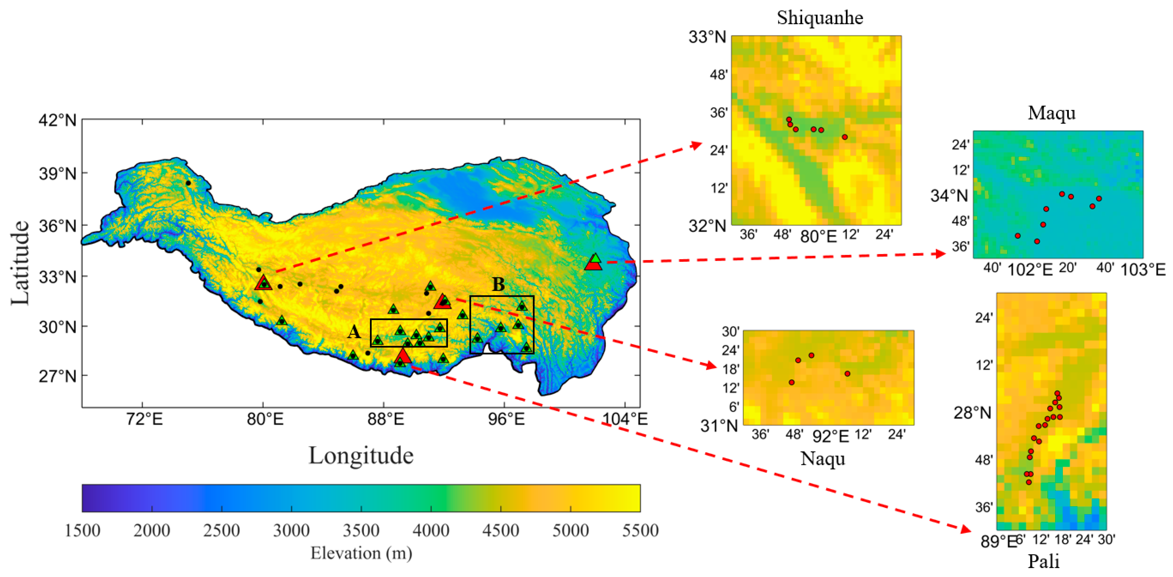
2.1.1. In situ Datasets

Detailed information on the in situ SM measurements during the non-frozen period from 2015 to 2016 is listed in

Table 1. Data sampling information of the in situ observations.

	Cover Period	Variable	Temporal Reso	Sites Number	Depth
TIPEX-III	2015–2016	SM	daily	32	0–10 cm
Pali	2015–2016	SM	1 h	16	0–5 cm
Shiquanhe	2015–2016	SM	15 min	6	0–5 cm
Naqu	2015–2016	SM	15 min	4	0–5 cm
Maqu	2015–2016	SM	15 min	8	0–5 cm
AWS	2015–2016	LST, Rainfall	daily	21	-

[23,28,29,30,31]. Note that the station-averaged SM is used to represent the SM reference data at each observing network. In addition to the in situ SM observations, the daily in situ rainfall and LST observations from Automatic Weather Stations (AWS) in the TP during the non-frozen period from 2015 to 2016 are also used in this study (Table 1).

2.1.2. Satellite Datasets

SMAP is the latest L-band satellite dedicated to providing a global-scale SM and freeze/thaw state. SMAP was launched on 31 January 2015 and carried two L-band microwave sensors, a radiometer, and a radar to sense soil conditions through moderate vegetation cover [18,24]. SMAP has been producing model-derived value-added Level 4 data to fill this gap with the root zone SM estimates, which are informed by and consistent with SMAP surface observations [32,33,34]. SMAP L4 observations are interpolated and extrapolated in time and space, producing 3-hour SM estimates at a 9 km resolution. SMAP L4 SM product provides a comprehensive and consistent picture of land surface hydrological conditions based on SMAP observations and complementary information from a variety of sources [33]. In this study, the surface SM of SMAP L4 Global 3-hourly 9 km EASE-Grid Surface and Root Zone Soil Moisture Analysis Update, Version 5 product (hereinafter referred to as SMAP) is adopted (

Table 2. Overview of the satellite, GLDAS, and reanalysis datasets used in this study.

	Variables	Cover Period	Temporal Reso	Spatial Reso	Depth
AMSR2	SM	2015–2016	daily	10 km	1–2 cm
SMAP	SM	2015–2016	15-min	9 km	3–5 cm
GLDAS-Noah	SM	2015–2016	15-min	0.25°	0–10 cm
ERA5	SM	2015–2016	hourly	0.25°	0–7 cm
MODIS	NDVI	2015–2016	16-day	250 m	-

).

AMSR2 as the successor of AMSR-E was on board the Global Change Observation Mission 1-Water (GCOM-W1) and launched on 18 May 2012 by the Japan Aerospace Exploration Agency (JAXA). AMSR2 has an antenna diameter of 2.0 m, an additional C-band (i.e., 7.3 GHz C2-band) channel to mitigate RFI, and an improvement in calibration accuracy through a modified thermal design [35]. AMSR2 observations are available twice daily, consisting of descending (01:30 local time) and ascending (13:30 local time) overpasses [36]. The daily GCOM-W1/AMSR2 SMC L3 standard product at 10 km × 10 km is evaluated in this study (Table 2). AMSR2 SM is combined from the ascending and descending observations in this study.

NDVI of the Moderate Resolution Imaging Spectroradiometer/Terra Vegetation Indices 16-Day L3 Global 250 m SIN Grid V006 (MOD13Q1) product is selected in this study [37] (Table 2).

2.1.3. GLDAS Product

The Global Land Data Assimilation System (GLDAS) is jointly developed by the National Aeronautics and Space Administration’s (NASA’s) Goddard Space Flight Center (GSFC) and the NCEP of the United States National Oceanic and Atmospheric Administration (NOAA). GLDAS products are produced by combining a huge quantity of observation-based data using advanced land surface modeling and data assimilation techniques. The four LSMs in the GLDAS system (i.e., NOAH, Community Land Model, Variable Infiltration Capacity, and MOSAIC) have simulated SM products with different spatial and temporal resolutions [16,38]. The surface layer SM (0–10 cm) from the GLDAS Noah Land Surface Model L4 3-hourly 0.25 × 0.25 degree V2.1 (hereinafter referred to as GLDAS-Noah) is used in our analysis (Table 2).

2.1.4. Reanalysis Product

ERA5 is the fifth and latest global climate reanalysis dataset produced by ECMWF, which provides hourly estimates of large numbers for atmospheric, land, and oceanic climate variables [39]. ERA5 is produced using 4D-Var data assimilation and model forecasts in CY41R2 of the ECMWF Integrated Forecast System (IFS), which improves with many modifications, representing a decade of research and development in modeling and data assimilation. The upper layer ERA5 SM (0–7 cm) is used in this study [10,16,40] (Table 2).

2.2. Methodology

2.2.1. Statistical Indices

Taking the in situ observed SM as the reference data, the statistical indices, including the nonparametric Spearman’s rank correlation ($\rho$), root mean square error (RMSE), bias (bias), and unbiased RMSE (ubRMSE) of SM products, are calculated to describe their performances in different seasons during the non-frozen period from 2015 to 2016 at regional and site scales in the TP.

$$\begin{array}{c}\rho =1-\frac{6{{\displaystyle \sum }}_{i=1}^N{\left(M_i-O_i\right)}^2}{N\left(N^2-1\right)}\end{array}$$

(1)

$$\begin{array}{c}RMSE=\sqrt{\frac{1}{N}{\displaystyle {\displaystyle \sum }_{i=1}^N}{\left(M_i-O_i\right)}^2}\end{array}$$

(2)

$$\begin{array}{c}bias=\frac{1}{N}{\displaystyle {\displaystyle \sum }_{i=1}^N}\left(M_i-O_i\right)\\ \end{array}$$

(3)

$$\begin{array}{c}ubRMSE=\sqrt{RMS{E}^2-bia{s}^2} \end{array}$$

(4)

where $M_i$ and $O_i$ are SM products and in situ observed SM, respectively. $\rho$ is a nonparametric measure of rank correlation measuring the strength and direction of association between SM products and in situ observed SM. The RMSE depicts the degree of deviation from different SM products. The bias represents the differences between the SM products and in situ SM observations. Note that RMSE (Equation (2)) could be compromised if there are biases associated with the amplitude fluctuations within SM products or in situ observations. Hence, ubRMSE is also adopted to evaluate the temporal dynamic variabilities of SM products in this study. The statistical metrics are calculated when the minimum sample size is equal to 30 in this study.

The spatial scale mismatch between the in situ observation point data and grid data is an issue. Since an interpolation method may produce a large error, the SM of various data sources is extracted from the original grids corresponding to each measurement station separately using the nearest neighboring grid approach (based on its latitude and longitude) [10,40,41]. To further reduce the error caused by the spatial scale mismatch, the extracted original grid data are averaged to produce the time series of the four SM products in each study region [15,17,21]. Besides, ubRMSE is used to avoid the effects of biases caused by the spatial scale mismatch between SM products and in situ observations in this study [18,40].

2.2.2. Multiple Linear Stepwise Regression

Multiple linear regression is one of the linear regression analyses that is used to analyze the relationship between a single response variable (dependent variable) and two or more controlled variables (independent variables) [42]. Compared with multiple linear regression analysis, stepwise regression has a more reasonable independent variable screening mechanism, which could avoid the influence of insignificant independent variables on the regression equation through forward selection and backward elimination [43]. The stepwise multiple regression method is able to find a meaningful subset of independent variables and explains the dependent variable efficiently. Therefore, the stepwise multiple regression analysis enables us to clearly comprehend the relationships between SM and the possible influencing factors [44]. The stepwisefit function of MATLAB is used to carry out the stepwise multiple regression analysis in this study (Equation (5)).

$$\begin{array}{c}\widehat{Y}=b_0+b_1{X}_1+b_2{X}_2+\dots +b_p{X}_p\end{array}$$

(5)

$$\begin{array}{c}{\beta }_i=\frac{std\left(X_i\right)}{std\left(\widehat{Y}\right)}, \left(i=1,2,3,\dots ,p\right)\end{array}$$

(6)

where $\widehat{Y}$ is the dependent variable. $X_1$ through $X_p$ are $p$ independent variables. $b_0$ is the value of $\widehat{Y}$ when all of the independent variables ($X_1$ through $X_p$) are equal to zero. $b_1$ through $b_p$ are the estimated regression coefficients. However, as the units of the independent variables are inconsistent, this makes the different regression coefficients incomparable. The standardized regression coefficient (β) (Equation (6)) could eliminate the influence of dimensional units of the independent variables. Then, the β values of different independent variables are comparable. Thus, β could directly reflect the influence degree of the independent variables, and further assess the effect, predictive power, or explanative power of an independent variable. In this study, β is adopted to analyze the associations between SM products and influencing factors (rainfall, NDVI, and LST).

3. Results

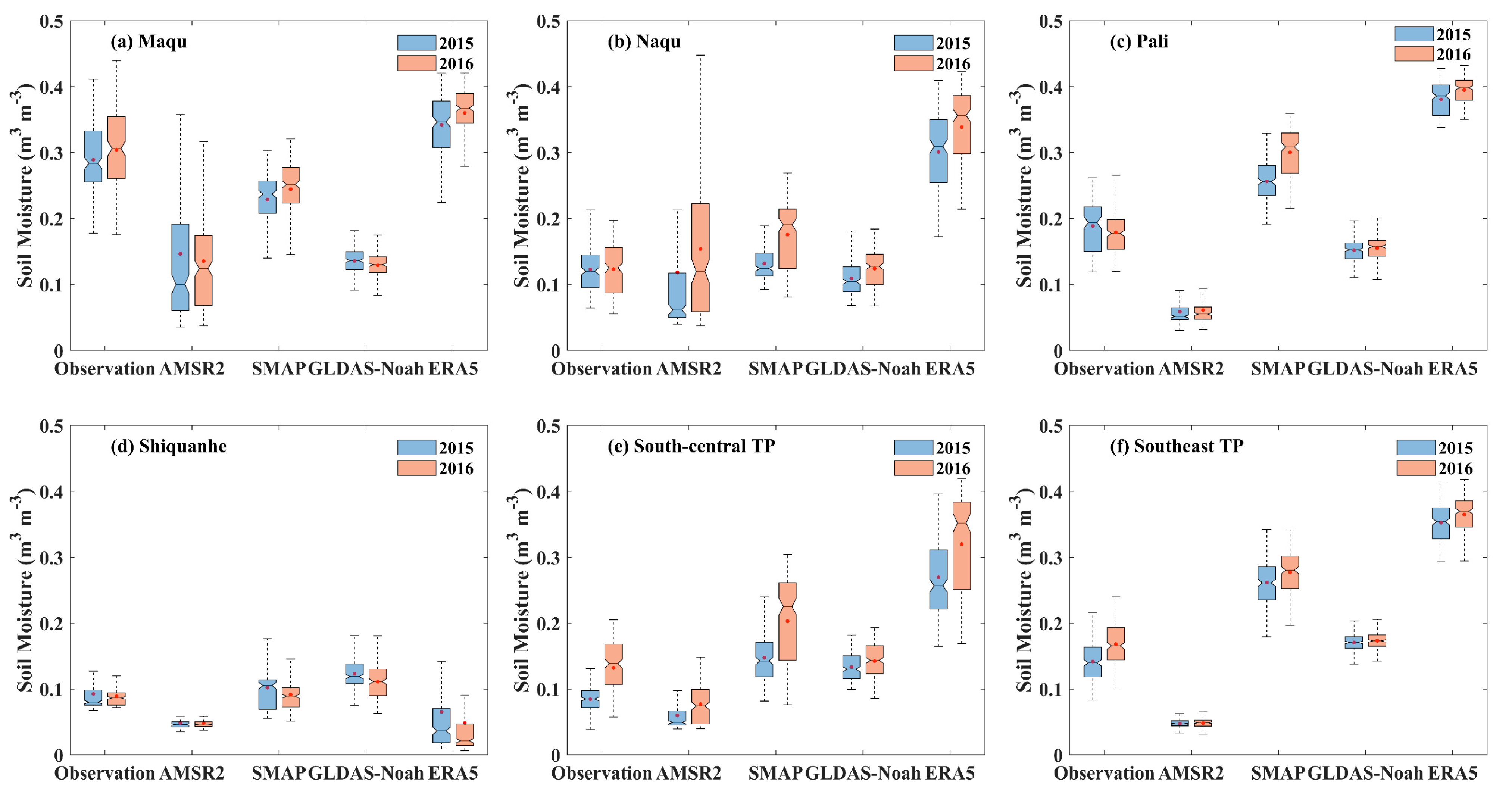
3.1. Tempo-Spatial Variations of the SM Observations

The time series and boxplots of the daily in situ observed SM in April–October during 2015–2016 in the TP are shown in Figure 2 and Figure 3. Here, the TIPEX-III SM measurement stations are mainly divided into two regions (TIPEX-III A: the south-central TP; TIPEX-III B: the southeast TP) (Figure 1). The averaged SM and rainfall observations in each region are calculated through the measured data at their overlapping stations in Figure 1.

The alpine humid climate in Maqu leads to its SM being larger than that in other observing networks. Its rainfall concentrates in May–September. The maximum SM is 0.41 m³/m³ (0.44 m³/m³) in September 2015 (August 2016) with the averaged value of 0.29 m³/m³ (0.31 m³/m³) during the non-frozen period in 2015 (2016). Naqu and Pali have a semi-arid monsoon climate, with averaged SM values above 0.12 m³/m³ during the study period. Their rainfall mainly concentrates in May–September. In Naqu, the maximum SM is 0.23 m³/m³ (0.20 m³/m³) on 25 June 2015 (13 July 2016). Note that its maximum rainfall (28.6 mm) occurs on 16 September 2016, but the maximum SM occurs in July. This may be caused by the rainfall intensity on 13 July 2016 being higher than that on 16 September 2016. In Pali, its maximum SM is 0.26 (0.31) m³/m³ on 8 August 2015 (25 July 2016). Shiquanhe is located in an arid climate zone and is covered by sparse grassland and bare soil. Its rainfall concentrates in June–August. The averaged SM value is 0.093 (0.089) m³/m³ during the non-frozen period in 2015 (2016). The maximum SM value is 0.18 m³/m³ on 11 July 2015 (Figure 3d). There are no obvious fluctuations in the in situ observed SM in April–May and September–October due to the low amount of rainfall (Figure 2d).

In addition to the in situ observed SM from the four observing networks above, the TIPEX-III SM observations are also analyzed in this study. The south-central TP has a plateau valley topography with a climate drier than central TP. Its rainfall concentration period (May–September) is the same as that in Naqu and Pali. However, the amount of rainfall is less than those in the above two regions (Figure not shown). The averaged SM is 0.12 m³/m³, which is comparable with that of Naqu and obviously less than that of Pali (Figure 3). The maximum SM (0.23 m³/m³) occurs on 28 July 2016 caused by its high rainfall intensity. Note that the averaged SM observation in 2015 is greater than that of Naqu and less than that of Pali, while the rainfall is the opposite (Figure 2). This indicates that the rainfall is not the only factor affected by SM in the south-central TP. Affected by the temperate–humid climate and topography in the southeast TP, rainfall occurs throughout the whole non-frozen period and is relatively larger than those in other TP regions. The averaged SM is 0.14 (0.17) m³/m³ in 2015 (2016) (Figure 3). The maximum value is 0.24 m³/m³ on 26 July 2016. Same as that in Maqu, the SM in southeast TP fluctuates obviously, which may be caused by the high frequency of rainfall.

The spatial distributions of the in situ observed SM in different seasons are shown in Figure 4. The in situ observed SM increases from northwest to southeast in the TP. The SM values are lower in April–May and September–October than those in June–August. Note that the averaged SM value at Shiquanhe is 0.09 m³/m³ during the study period. However, at the Shiquanhe network, the averaged SM value (0.19 m³/m³) at the SQ04 station is larger than those in other sites, which may be due to its underlying surface type being wetland (Figure 4(a1–d1)). Similarly, at the Maqu network, the SM at the NST05 station is greater than those in other stations, which may be also caused by its different local underlying surface type.

3.2. Comparison among Different SM Products

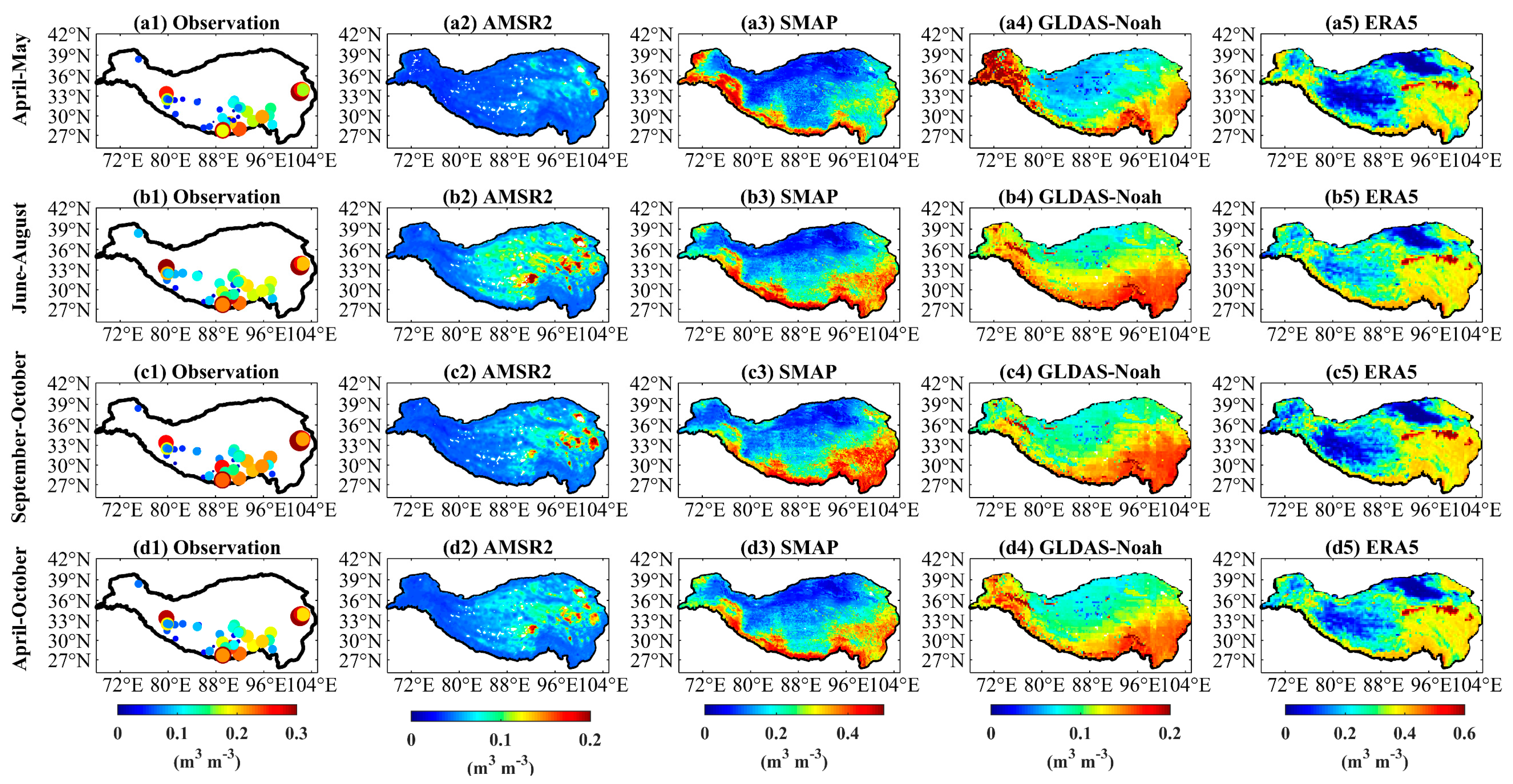
3.2.1. Tempo-Spatial Variations of SM Products

Similar to the in situ observed SM, there are obvious seasonal variations for AMSR2, SMAP, GLDAS-Noah, and ERA5 SM during the study period, especially in the summer (Figure 2). SMAP SM captures the seasonal variations of the in situ observed SM well at all regions, with the correlations greater than 0.55, ubRMSEs lower than 0.042 m³/m³ (Figure 2 and Figure 5). In Maqu, SMAP SM slightly underestimates the observations with the $\rho$ of 0.74 and ubRMSE of 0.037 m³/m³ (Figure 2 and Figure 5). The performance of ERA5 SM is slightly second to that of SMAP SM. In Naqu, the ubRMSEs of SMAP and ERA5 SM are around 0.041 m³/m³. The correlation between ERA5 SM and in situ observation is highest (0.77). In Pali, for SMAP and ERA5 SM, the correlations between them and the in situ observed SM are comparable, with the $\rho$ values around 0.55. ERA5 SM has the lowest ubRMSE of 0.029 m³/m³ (Figure 2 and Figure 5). In Shiquanhe, SMAP and GLDAS-Noah SM have the highest $\rho$ values of 0.66. The GLDAS-Noah SM slightly underestimates the observations with the lowest ubRMSE of 0.020 m³/m³ (Figure 5). For AMSR2 SM, it seriously overestimates (underestimates) the in situ observed SM during the periods with large (less) quantities of rainfall in Maqu and Naqu (Figure 2b and Figure 3b). The ubRMSEs of AMSR2 SM in the above two regions are greater than 0.08 m³/m³. GLDAS-Noah SM present serious underestimation with the bias value of −0.16 m³/m³ and a small $\rho$ value in Maqu (Figure 5). Except for Maqu, GLDAS-Noah SM values are closer to in situ observed SM values than those of other SM products with the small ubRMSEs and biases. However, its $\rho$ values are relatively low in Naqu and Pali observing networks (Figure 2, Figure 3 and Figure 5).

In terms of the TIPEX-III observations, the variations of the four SM products agree well with those of in situ SM observations in south-central TP, with correlations greater than 0.59 (Figure 2, Figure 3 and Figure 5). SMAP SM has a maximum $\rho$ of 0.92 and the smallest ubRMSE of 0.028 m³/m³ among the four SM products. AMSR2 and GLDAS-Noah SM also capture the in situ observed SM values with the ubRMSEs of 0.030 and 0.033 m³/m³, respectively. In southeast TP, the seasonal variations of AMSR2 SM are relatively flat (Figure 2f and Figure 3f). ERA5 SM has the highest $\rho$ (0.76) and smallest ubRMSE (0.022 m³/m³) among the four SM products. The $\rho$ value of SMAP SM is 0.60, behind that of ERA5 SM. For AMSR2 and GLDAS-Noah SM, their consistencies with the in situ SM observations are poor, with correlations around 0.51.

Figure 6 shows the scatterplots between the four SM products and in situ observed SM in the TP in different seasons during the non-frozen period from 2015 to 2016. The $\rho$ values of the four SM products are lowest in April–May, and highest in September–October. SMAP and ERA5 SM have bias values greater than 0.043 and 0.12 m³/m³ in all the seasons, respectively (Figure 6). The results indicate that ERA5 SM seriously overestimates the in situ observations, especially during the summer. This may be due to ERA5 LST showing an underestimation with a bias about −9.5 K during the study period in the TP (Figure not shown). The seasonal variations of the in situ observed SM are well captured by those of SMAP and ERA5 SM with the $\rho$ values greater than 0.81 during the entire study period (Figure 6). Meanwhile, AMSR2 and GLDAS-Noah SM underestimate the in situ observed SM with bias values less than −0.010 m³/m³. Although GLDAS-Noah SM values are closer to in situ observed SM values than those of other SM products, the correlations between them and in situ observations are relatively low in all study periods. Note that although SMAP and ERA5 (AMSR2) SM are sometimes lower (higher) than the in situ observations in different study regions (Figure 2), they overestimate (underestimate) the in situ observations for the average across all measurement sites in the TP during the study period (Figure 6).

The spatial distributions of the four SM products are also given in Figure 3. The lowest (largest) values of SMAP, GLDAS-Noah, and ERA5 SM are found in western TP and the Qaidam Basin in northern TP (south and eastern TP). In contrast with the three SM products above, AMSR2 SM has the lowest values in northwest TP and southeast TP. ERA5 SM obviously overestimates the in situ observations in eastern TP. AMSR2 and GLDAS-Noah SM obviously underestimate the in situ observations in the whole TP (Figure 3). In general, the spatial distributions of SMAP and ERA5 SM are well consistent with those of in situ observations at the site scale in the TP during the study periods.

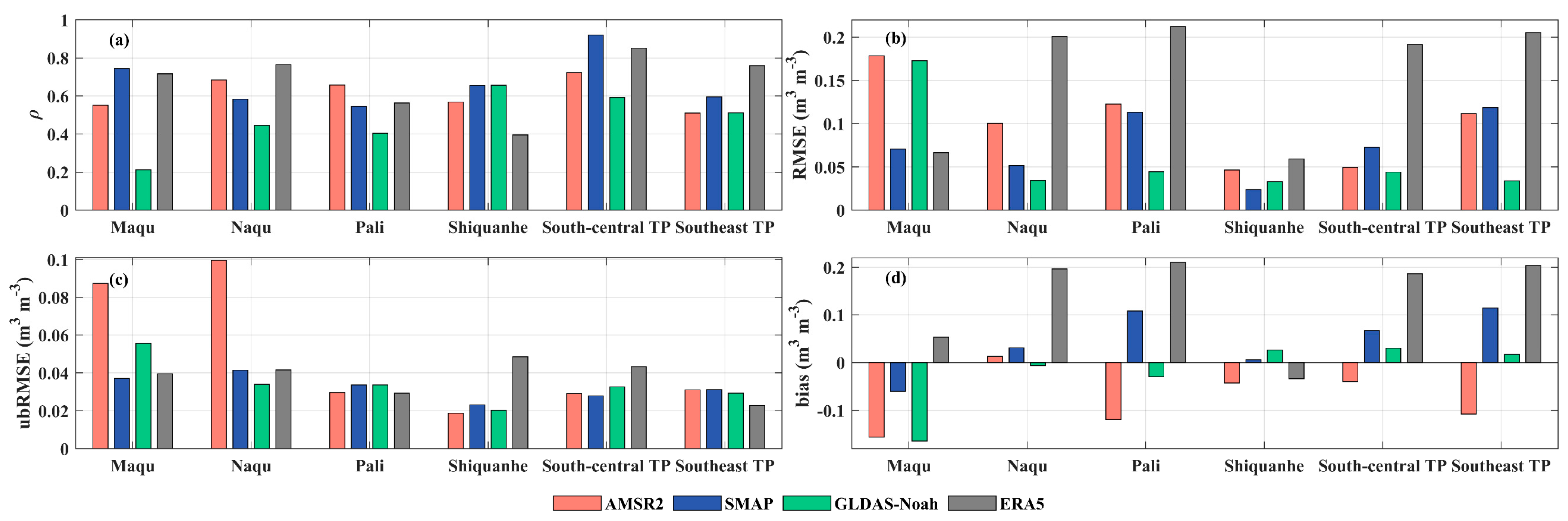
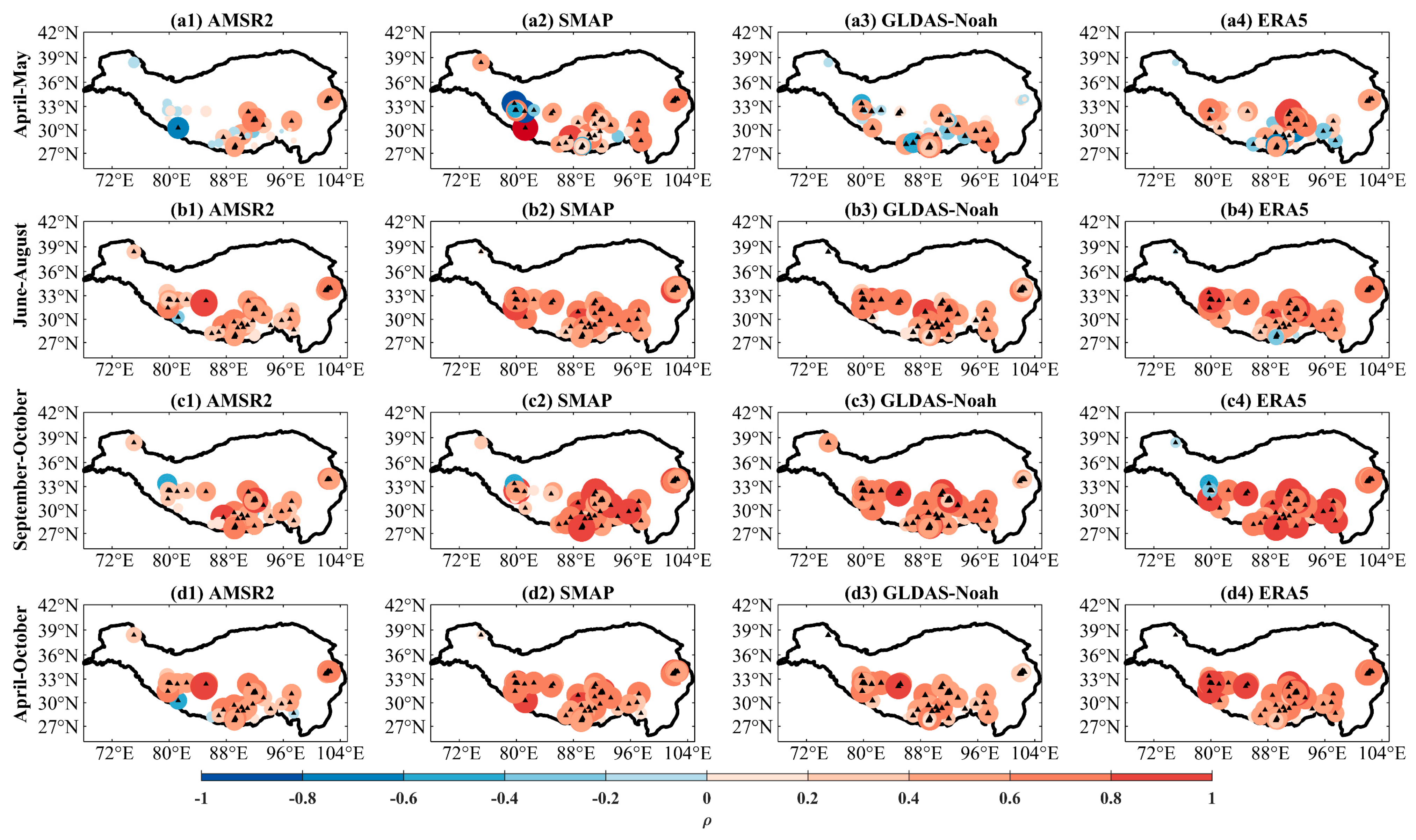
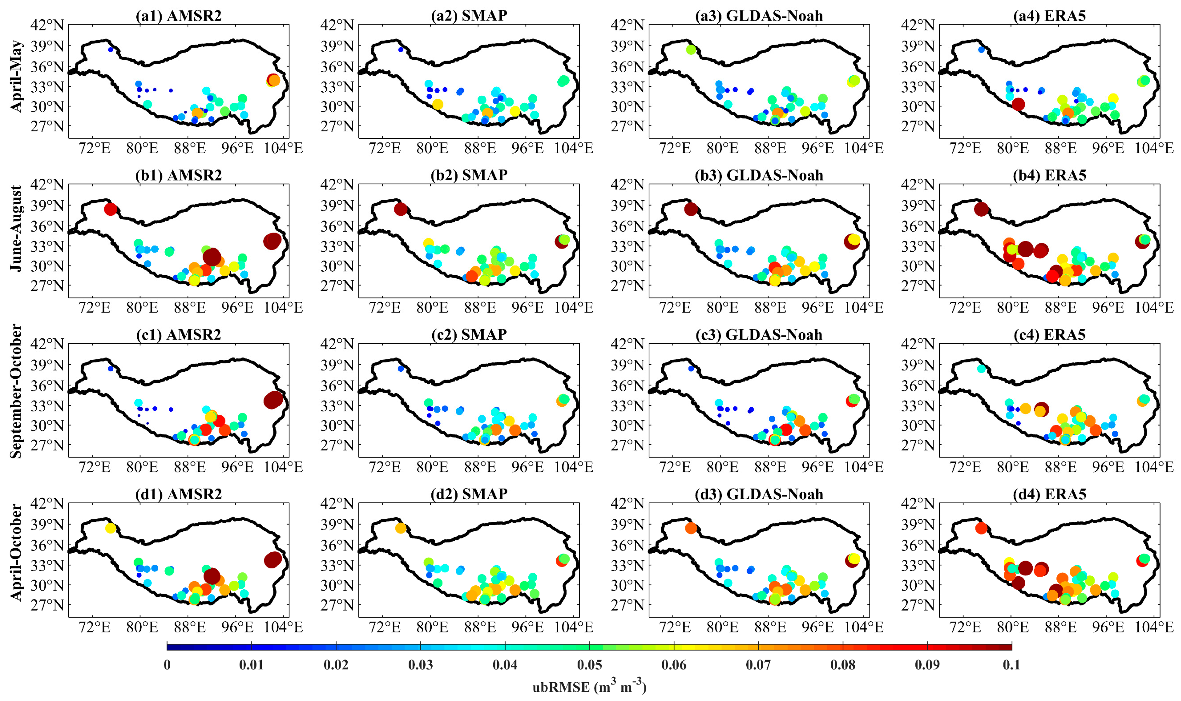
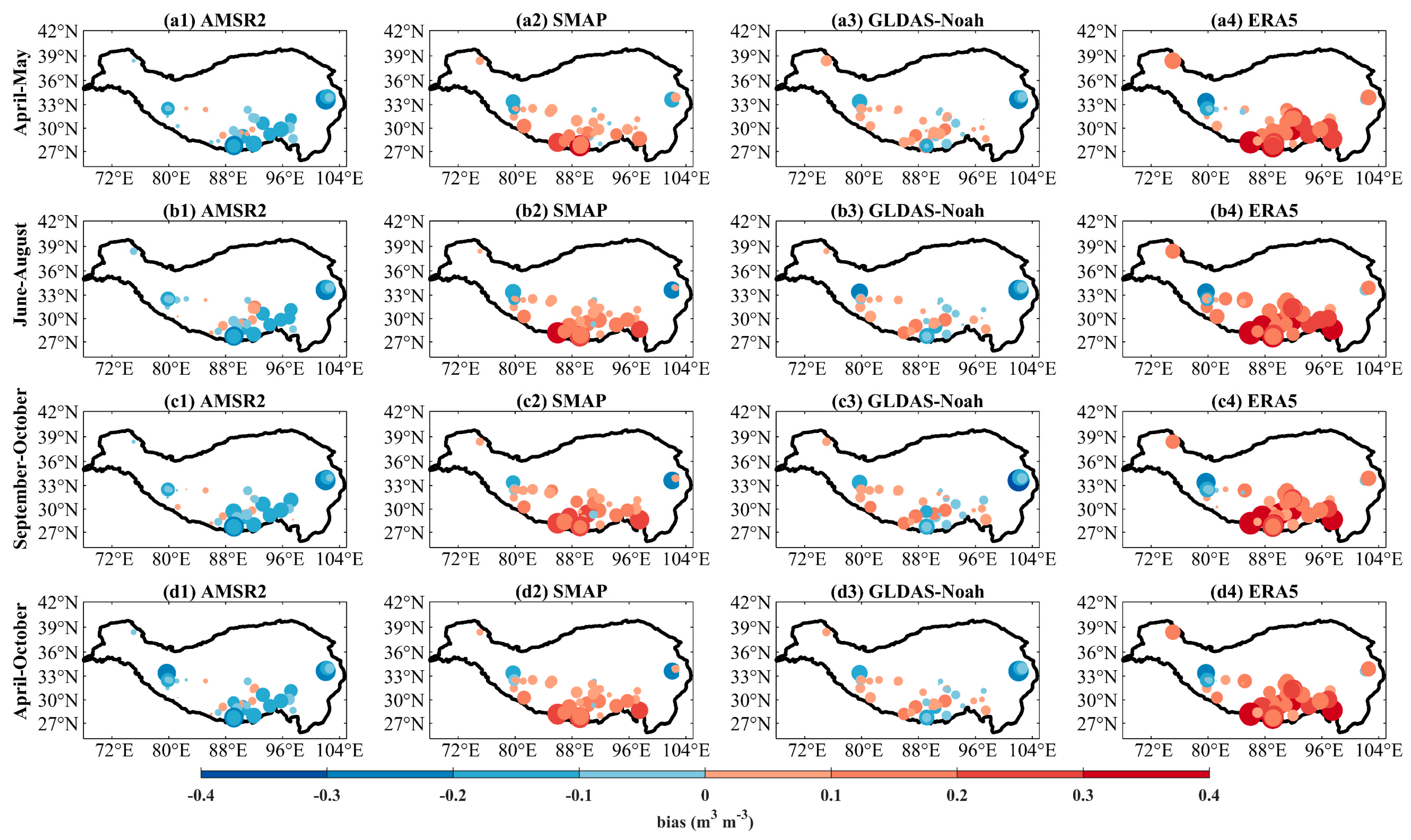
3.2.2. Spatial Distributions of Statistical Indices for SM Products

The spatial distributions of the statistical indices ($\rho$, ubRMSE, and bias) for AMSR2, SMAP, GLDAS-Noah, and ERA5 SM at 66 TP observation stations in different seasons during the study period are shown in Figure 7, Figure 8 and Figure 9.

At the site scale, the significant positive correlations between the four SM products and in situ measured SM are between 0.19 and 0.88 in April–May and between 0.15 and 0.89 in June–August. In April–May, the $\rho$ value between AMSR2/GLDAS-Noah/ERA5 SM and in situ observed SM is relatively low, which may be due to the number of stations with significant correlations being less than 46% (

Table 3. The number of sites with positive correlation (statistically significant at 95% confidence level) between the four SM products (AMSR2, SMAP, GLDAS-Noah, and ERA5 SM) and in situ observed SM in different seasons during the non-frozen period from 2015 to 2016.

Periods	AMSR2	SMAP	GLDAS-Noah	ERA5
April–May	24	40	29	32
June–August	58	59	61	55
September–October	52	56	59	56
April–October	57	62	62	63

). Meanwhile, the $\rho$ value of GLDAS-Noah (AMSR2) SM with in situ observation is lowest among the four SM products in April–May (June–August) in terms of TP regional mean. In general, SMAP (GLDAS-Noah) SM has better correlations with in situ observations than other SM products at most stations in April–May (June–August) (Table 3). In September–October, the number of sites with positive correlations of GLDAS-Noah/SMAP/ERA5 SM between in situ observations are greater than those for AMSR2 SM. The regional mean $\rho$ values of AMSR2, SMAP, GLDAS-Noah, and ERA5 SM are 0.50, 0.95, 0.56, and 0.93, respectively. Obviously, SMAP and ERA5 SM correlate well with in situ observations in east-central TP (Figure 7). During the whole study period, the number of stations with significant correlations for SMAP/GLDAS-Noah/ERA5 SM between in situ observations are comparable, which is greater than that for AMSR2 (Table 3). The regional mean $\rho$ values of AMSR2, SMAP, GLDAS-Noah, and ERA5 SM are 0.56, 0.85, 0.57, and 0.81, respectively. Meanwhile, the $\rho$ values of the four SM products in the Karakoram Mountains and Himalayan Mountains are lower than those in other TP regions (Figure 7).

As shown in Figure 8, the spatial distributions of the ubRMSE values in different seasons for each SM dataset are generally consistent. For AMSR2, SMAP, and GLDAS-Noah SM, the small ubRMSE (<0.05 m³/m³) regions are located in most central, western, and southeastern TP. In Maqu, the above three SM products present large ubRMSE values, which mainly reflects in the negative bias values of them (Figure 9). This may be caused by the in situ observed SM being relatively large at the NST05 station in the Maqu network (Figure 4(a1–d1)), which is barely captured by the above three SM products. The AMSR2 SM also has large ubRMSEs in Naqu. This is possible because of the large AMSR2 SM values during the rainfall period (Figure 2 and Figure 8). For SMAP SM, there are obviously positive bias values in the Himalayas region and negative bias values in Shiquanhe and Maqu. For ERA5 SM, the ubRMSE values are obviously larger than those of the other three SM products at the most stations in the TP, especially in central and south-central TP. Meanwhile, there are positive bias values for ERA5 SM in central and south-central TP, with a maximum value of 0.38 m³/m³ in summer (Figure 9). ERA5 SM also shows an underestimation in Shiquanhe. Generally, except for the Karakoram Mountains and Himalayan Mountains, SMAP SM has a relatively high $\rho$ and low ubRMSE values at the most stations in the TP (Figure 8). Meanwhile, compared with the RMSE values of SMAP L3, those of SMAP L4 in this study are relatively small [18,24].

Note that the discrepancies in the depth of the soil layer represented by the satellite, LSMs and reanalysis datasets may affect the accuracy of the SM products in this study. For example, AMSR2 SM is more sensitive to rainfall than other SM products in Naqu and Shiquanhe, which may be caused by the penetration depth of the X-band and C-band radiometers for AMSR2 being shallow (1–2 cm). The penetration depth of ERA5 SM is 0–7 cm, which may be another reason for its serious overestimation at the observing networks. For GLDAS-Noah and SMAP SM, the influence of SM penetration depth is not as significant as the other two SM products.

4. Discussion

The above results indicate that the four SM products have deviations in different degrees during the non-frozen period from 2015 to 2016 in the TP. Previous studies show that the rainfall, land surface types, and temperatures are the main error sources in SM from satellite and reanalysis datasets [11,45]. In order to investigate the main influencing factors for the four SM products in this study, the rainfall, NDVI, and LST are selected. To ensure the accuracy of the correlation analysis and the multiple linear stepwise regression analysis, the following study is conducted at the stations with in situ SM, rainfall, and LST observations.

The rainfall, NDVI, and LST gradually increase from northeast to southwest in all seasons in the TP, which is spatially consistent with the distributions of in situ observed SM. The maximum (minimum) values of rainfall, NDVI, and LST occur in June–August (April–May) (Figure 10). The high values of rainfall and NDVI are located in eastern TP. For LST, the high values are mainly located in eastern and northern TP in the summer and in eastern TP in other seasons.

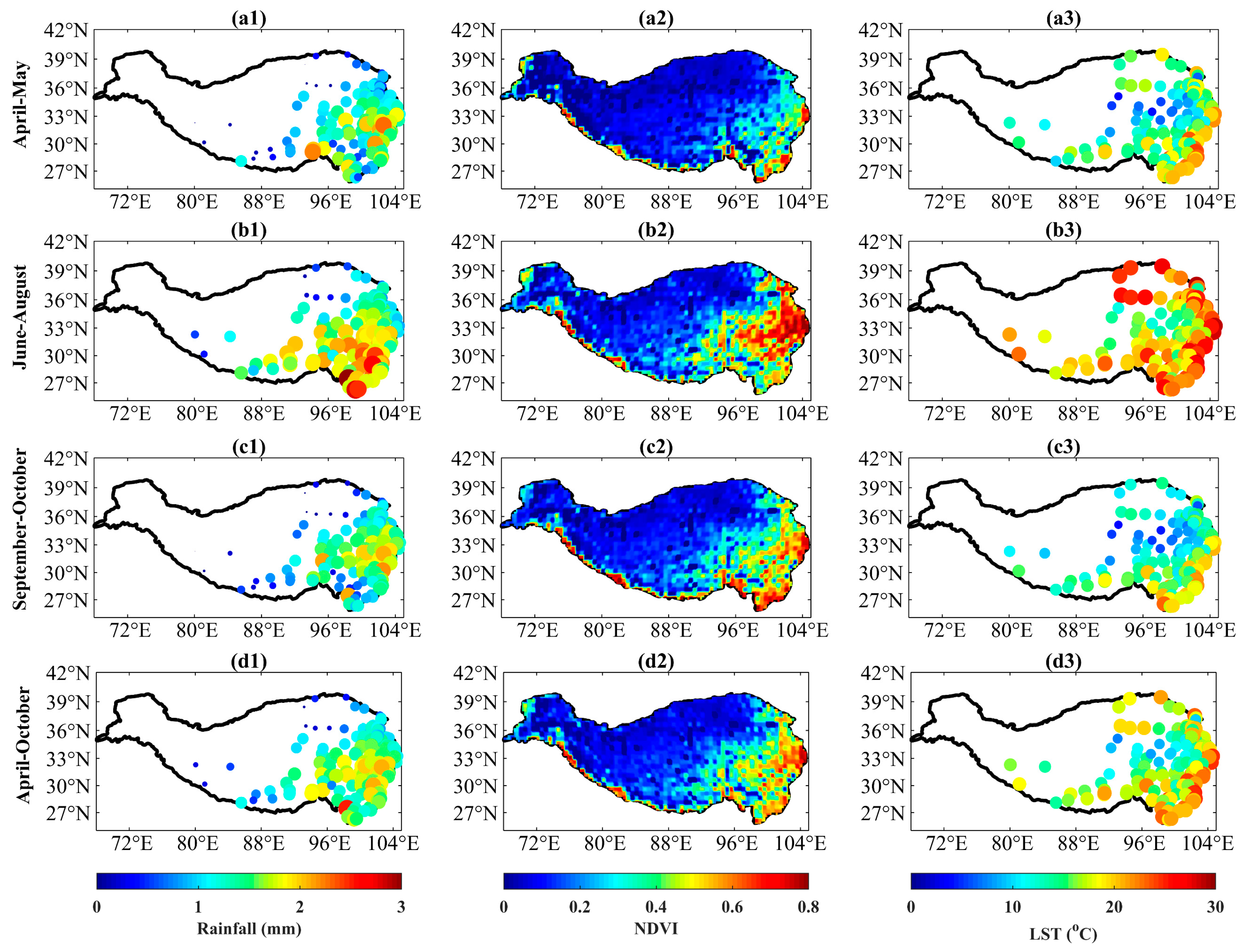
4.1. The Correlations between SM and the Influencing Factors

The correlations between in situ observed SM and the three factors are given in

Table 4. The $\rho$ between SM (in situ observation, AMSR2, SMAP, GLDAS-Noah, and ERA5) and influencing factors (rainfall, NDVI, and LST) in different seasons from 2015 to 2016 in the TP. *, **, and *** represent the statistically significant at 95%, 99%, and 99.9% confidence levels, respectively.

Periods	Variables	Observations	AMSR2	SMAP	GLDAS-Noah	ERA5
April–May	Rainfall	0.31 ***	0.26 **	0.27 **	0.02	0.10
	NDVI	0.31 ***	0.56 ***	0.23 *	0.16	0.56 ***
	LST	0.16	0.48 ***	0.21 *	0.28 **	0.54 ***
June–August	Rainfall	0.45 ***	0.68 ***	0.55 ***	0.46 ***	0.61 ***
	NDVI	0.15 *	−0.047	0.30 ***	0.36 ***	0.12
	LST	−0.56 ***	−0.59 ***	−0.56 ***	−0.38 ***	−0.64 ***
September–October	Rainfall	0.55 ***	0.76 ***	0.73 ***	0.74 ***	0.69 ***
	NDVI	0.41 ***	0.75 ***	0.58 ***	0.91 ***	0.45 ***
	LST	0.22 *	0.64 ***	0.40 ***	0.81 ***	0.45 ***
April–October	Rainfall	0.46 ***	0.64 ***	0.48 ***	0.48 ***	0.58 ***
	NDVI	0.52 ***	0.68 ***	0.65 ***	0.71 ***	0.64 ***
	LST	0.18 ***	0.52 ***	0.23 ***	0.42 ***	0.39 ***

. For the whole study period, the $\rho$ value (0.52) between in situ observed SM and NDVI is best. In April–May and September–October, NDVI and rainfall, respectively, have the highest correlations with in situ observed SM, with the $\rho$ values of 0.31 and 0.55, respectively. For LST, there is a significant negative correlation ($\rho$ = −0.56) in June–August and positive correlations in other seasons. The negative $\rho$ values in the summer may be due to the frequent rainfall, which results in the saturation of SM. The summer LST is relatively higher than that in other seasons, which facilitates surface evaporation and reduces local SM. In April–May (September–October), the increase (decrease) in LST and rainfall leads to the increased (decreased) SM (Table 4).

Table 4 further shows the correlations between the four SM products and the three influencing factors. There are significant positive correlations between the four SM products and the three influencing factors during the whole study period, especially with NDVI (Table 4). In April–May, AMSR2 and ERA5 SM have the highest positive correlations with NDVI, the next being with LST. There is a significant positive relationship between SMAP SM and rainfall. Meanwhile, GLDAS-Noah SM has a significant positive correlation with LST. In the summer, similar to in situ observed SM, SMAP and ERA5 SM have the highest negative correlations with LST. AMSR2 and GLDAS-Noah SM have the highest positive correlations with rainfall, which implies that they are highly sensitive to the rainfall (Figure 2b). In September–October, the relationships between AMSR2/SMAP/ERA5 SM and rainfall have the highest $\rho$. GLDAS-Noah SM has the best correlations with NDVI.

4.2. The Main Factors Influencing SM

To explore the main influencing factors of SM datasets in this study, the multiple linear stepwise regression is used.

Table 5. The β from multiple stepwise regression analysis between SM (in situ observed, AMSR2, SMAP, GLDAS-Noah, and ERA5) and influencing factors (rainfall, NDVI, and LST) in different seasons from 2015 to 2016 in the TP. *, **, and *** represent the statistically significant at 95%, 99%, and 99.9% confidence levels, respectively.

Period	Variables	Observations	AMSR2	SMAP	GLDAS-Noah	ERA5
April–May	Rainfall	0.33 ***	0.44 ***	0.51 ***	0.37 ***	0.07
	NDVI	−0.09	−0.02	−0.33 *	−0.45 **	0.55 ***
	LST	0.39 ***	0.57 ***	0.59 ***	0.76 ***	0.23
June–August	Rainfall	0.05	0.43 ***	0.22 **	0.29 ***	0.24 **
	NDVI	0.22 ***	0.01	0.36 ***	0.57 ***	0.19 ***
	LST	−0.56 ***	−0.30 ***	−0.45 ***	−0.16 *	−0.50 ***
September–October	Rainfall	0.45 ***	0.58 ***	0.56 ***	0.40 ***	0.37 ***
	NDVI	0.60 ***	0.10	0.41 ***	0.20 ***	0.53 ***
	LST	−0.37 ***	0.40 ***	−0.12	0.54 ***	−0.04
April–October	Rainfall	0.25 ***	0.55 ***	0.32 ***	0.29 ***	0.39 ***
	NDVI	0.67 ***	0.24 ***	0.71 ***	0.58 ***	0.53 ***
	LST	−0.37 ***	0.18 ***	−0.31 ***	−0.03	0.01

gives the regional mean β between SM datasets and the three factors (rainfall, NDVI, and LST) in different seasons during the study period.

In April–May, rainfall and LST are the main influencing factors to SM of in situ observation, AMSR2, SMAP, and GLDAS-Noah, with β greater than 0.33. ERA5 SM is mainly affected by NDVI (β = 0.55). In contrast with the correlations, the β results indicate that neglecting the influence of rainfall and NDVI makes LST the main influencing factor on most SM datasets in the spring. In the summer, for in situ observed, SMAP, and ERA5 SM, LST is the dominant negative influencing factor, which is consistent with the results of the correlation reanalysis. For AMSR2 and GLDAS-Noah SM, the main influencing factors are rainfall (β = 0.43) and NDVI (β = 0.50), respectively. In September–October, LST has a significant negative effect on in situ observed SM. NDVI is the main influencing factor for in situ observed and ERA5 SM. AMSR2 and SMAP (GLDAS-Noah) SM are mainly affected by rainfall (LST) with β values around 0.57 (0.54). This further illustrates the sensitivity of AMSR2 SM to rainfall. During the whole study period, rainfall, NDVI, and LST had different effects on the five SM datasets in different seasons. On the whole, the rainfall and NDVI have the most significant positive effects on SM in this study.

5. Conclusions

The results in this study show that the temporal variation characteristics of in situ observed SM are various for different climate regions in the TP. The averaged SM values in different study regions from high to low in order is: Maqu, Pali, southeast TP, Naqu, south-central TP, and Shiquanhe, with obvious fluctuations in the summer. The maximum values of in situ observed SM occur in August–September, June–July, July–August, and July in Maqu, Naqu, Pali, and Shiquanhe, respectively. For TIPEX-III observations, the maximum SM values in south-central and southeast TP both occur in July. Meanwhile, the peak SM values occur later than the peak rainfall values in all study regions.

Compared with in situ observed SM, SMAP and ERA5 SM present an overestimation with the bias values of 0.057 and 0.14 m³/m³, respectively. AMSR2 and GLDAS-Noah SM show an underestimation with the bias values of −0.069 and −0.010 m³/m³ during the whole study period. Besides, the performances of different SM products vary in different TP regions. For the alpine humid Maqu region, SMAP and ERA5 SM perform well and are comparable. In south-central TP, SMAP SM agrees well with the in situ observed SM. In Naqu, Pali, and southeast TP, ERA5 SM has a relatively high $\rho$ and the lowest ubRMSE values. In Shiquanhe, GLDAS-Noah SM is closest to the in situ observations. It is worth noting that the $\rho$ values of SMAP and ERA5 SM are relatively high, which may imply that there are obvious systematic deviations in them.

Generally, rainfall and NDVI present significant positive correlations with the five SM datasets during the study period in this study. LST has significant negative (positive) correlations with SM datasets in the summer (other seasons). The $\rho$ values between rainfall/NDVI and SM datasets are relatively larger than those between LST and SM datasets. AMSR2 SM is mainly influenced by rainfall, followed by NDVI. Except for AMSR2, the other SM datasets are mainly affected by NDVI (β > 0.53) in the TP. Meanwhile, in situ observed and SMAP SM are also affected by LST with negative β values. This indicates that neglecting the influence of NDVI and rainfall, LST has a negative effect on the two SM datasets above. Among the three influencing factors, rainfall and NDVI are identified as the two main influencing factors on the five SM datasets in this study, which is generally consistent with the correlation analysis.

References

1. Liu, Y.; Bao, Q.; Duan, A.; Qian, Z.; Wu, G. Recent progress in the impact of the Tibetan Plateau on climate in China. Adv. Atmos. Sci. 2007, 24, 1060–1076. [Google Scholar] [CrossRef]
2. Yang, K.; Guo, X.; He, J.; Qin, J.; Koike, T. On the climatology and trend of the atmospheric heat source over the Tibetan Plateau: An experiments-supported revisit. J. Clim. 2011, 24, 1525–1541. [Google Scholar] [CrossRef]
3. Zhao, P.; Xu, X.; Chen, F.; Guo, X.; Zheng, X.; Liu, L.; Hong, Y.; Li, Y.; La, Z.; Peng, H.; et al. The third atmospheric scientific experiment for understanding the earth-atmosphere coupled system over the Tibetan Plateau and its effects. Bull. Am. Meteorol. Soc. 2018, 99, 757–776. [Google Scholar] [CrossRef]
4. Lu, H.; Koike, T.; Yang, K.; Hu, Z.; Xu, X.; Rasmy, M.; Kuria, D.; Tamagawa, K. Improving land surface soil moisture and energy flux simulations over the Tibetan plateau by the assimilation of the microwave remote sensing data and the GCM output into a land surface model. Int. J. Appl. Earth Obs. 2012, 17, 43–54. [Google Scholar] [CrossRef]
5. Talib, J.; Taylor, C.; Duan, A.; Turner, A.G. Intraseasonal soil moisture-atmosphere feedbacks on the Tibetan Plateau circulation. J. Clim. 2021, 34, 1789–1807. [Google Scholar] [CrossRef]
6. Tian, J.; Qin, J.; Yang, K.; Zhao, L.; Chen, Y.; Lu, H.; Li, X.; Shi, J. Improving surface soil moisture retrievals through a novel assimilation algorithm to estimate both model and observation errors. Remote Sens. Environ. 2022, 269, 112802. [Google Scholar] [CrossRef]
7. Zhang, P.; Zheng, D.; Velde, R.; Wen, J.; Zeng, Y.; Wang, X.; Wang, Z.; Chen, J.; Su, Z. Status of the Tibetan Plateau observatory (Tibet-Obs) and a 10-year (2009–2019) surface soil moisture dataset. Earth Syst. Sci. Data 2021, 13, 3075–3102. [Google Scholar] [CrossRef]
8. Zhuang, R.; Zeng, Y.; Manfreda, S.; Su, Z. Quantifying long-term land surface and root zone soil moisture over Tibetan Plateau. Remote Sens. 2020, 12, 509. [Google Scholar] [CrossRef] [Green Version]
9. Cheng, M.; Zhong, L.; Ma, Y.; Zou, M.; Ge, N.; Wang, X.; Hu, Y. A study on the assessment of multi-source satellite soil moisture products and reanalysis data for the Tibetan Plateau. Remote Sens. 2019, 11, 1196. [Google Scholar] [CrossRef] [Green Version]
10. Yang, S.; Li, R.; Wu, T.; Hu, G.; Xiao, Y.; Du, Y.; Zhu, X.; Ni, J.; Ma, J.; Zhang, Y.; et al. Evaluation of reanalysis soil temperature and soil moisture products in permafrost regions on the Qinghai-Tibetan Plateau. Geoderma 2020, 377, 114583. [Google Scholar] [CrossRef]
11. Ling, X.; Huang, Y.; Guo, W.; Wang, Y.; Chen, C.; Qiu, B.; Ge, J.; Qin, K.; Xue, Y.; Peng, J. Comprehensive evaluation of satellite-based and reanalysis soil moisture products using in situ observations over China. Hydrol. Earth Syst. Sci. 2021, 25, 4209–4229. [Google Scholar] [CrossRef]
12. Liu, W.; Wang, J.; Xu, F.; Li, C.; Xian, T. Validation of four satellite-derived soil moisture products using ground-based in situ observations over northern China. Remote Sens. 2022, 14, 1419. [Google Scholar] [CrossRef]
13. Ming, W.; Ji, X.; Zhang, M.; Li, Y.; Liu, C.; Wang, Y.; Li, J. A hybrid triple collocation-deep learning approach for improving soil moisture estimation from satellite and model-based data. Remote Sens. 2022, 14, 1744. [Google Scholar] [CrossRef]
14. Wang, Y.; Leng, P.; Peng, J.; Marzahn, P.; Ludwig, R. Global assessments of two blended microwave soil moisture products CCI and SMOPS with in-situ measurements and reanalysis data. Int. J. Appl. Earth Obs. 2021, 94, 102234. [Google Scholar] [CrossRef]
15. Wang, Y.; Li, G. Evaluation of simulated soil moisture from China Land Data Assimilation System (CLDAS) land surface models. Remote Sens. Lett. 2020, 11, 1060–1069. [Google Scholar] [CrossRef]
16. Wu, Z.; Feng, H.; He, H.; Zhou, J.; Zhang, Y. Evaluation of soil moisture climatology and anomaly components derived from ERA5-land and GLDAS-2.1 in China. Water Resour. Manag. 2021, 35, 629–643. [Google Scholar] [CrossRef]
17. Bi, H.; Ma, J.; Zheng, W.; Zeng, J. Comparison of soil moisture in GLDAS model simulations and in situ observations over the Tibetan Plateau. J. Geophys. Res. Atmos. 2016, 121, 2658–2678. [Google Scholar] [CrossRef] [Green Version]
18. Chen, Y.; Yang, K.; Qin, J.; Qin, J.; Cui, Q.; Lu, H.; La, Z.; Han, M.; Tang, W. Evaluation of SMAP, SMOS, and AMSR2 soil moisture retrievals against observations from two networks on the Tibetan Plateau. J. Geophys. Res. Atmos. 2017, 122, 5780–5792. [Google Scholar] [CrossRef]
19. Dente, L.; Su, Z.; Wen, J. Validation of SMOS soil moisture products over the Maqu and Twente regions. Sensors 2012, 12, 9965–9986. [Google Scholar] [CrossRef]
20. Kang, J.; Jin, R.; Li, X.; Zhang, Y. Error decomposition of remote sensing soil moisture products based on the triple-collocation method introducing an unbiased reference dataset: A case study on the Tibetan Plateau. Remote Sens. 2020, 12, 3087. [Google Scholar] [CrossRef]
21. Zeng, J.; Li, Z.; Chen, Q.; Bi, H.; Qiu, J.; Zou, P. Evaluation of remotely sensed and reanalysis soil moisture products over the Tibetan Plateau using in-situ observations. Remote Sens. Environ. 2015, 163, 91–110. [Google Scholar] [CrossRef]
22. Zhang, Q.; Fan, K.; Singh, V.; Sun, P.; Shi, P. Evaluation of remotely sensed and reanalysis soil moisture against in situ observations on the Himalayan-Tibetan Plateau. J. Geophys. Res. Atmos. 2018, 123, 7132–7148. [Google Scholar] [CrossRef]
23. Dente, L.; Vekerdy, Z.; Wen, J.; Su, Z. Maqu network for validation of satellite-derived soil moisture products. Int. J. Appl. Earth Obs. 2012, 17, 55–65. [Google Scholar] [CrossRef]
24. Li, C.; Lu, H.; Yang, K.; Han, M.; Wright, J.S.; Chen, Y.; Yu, L.; Xu, S.; Huang, X.; Gong, W. The evaluation of SMAP enhanced soil moisture products using high-resolution model simulations and in-situ observations on the Tibetan Plateau. Remote Sens. 2018, 10, 535. [Google Scholar] [CrossRef] [Green Version]
25. Li, N.; Zhao, P.; Wang, J.; Deng, Y. Estimation of surface heat fluxes over the central Tibetan Plateau using the maximum entropy production model. J. Geophys. Res. Atmos. 2019, 124, 6827–6840. [Google Scholar] [CrossRef] [Green Version]
26. Li, Z.; Yu, G.; Xiao, X.; Li, Y.; Zhao, X.; Ren, C.; Zhang, L.; Fu, Y. Modeling gross primary production of alpine ecosystems in the Tibetan Plateau using MODIS images and climate data. Remote Sens. Environ. 2007, 107, 510–519. [Google Scholar] [CrossRef]
27. Ma, Y.; Hu, Z.; Xie, Z.; Ma, W.; Wang, B.; Chen, X.; Li, M.; Zhong, L.; Sun, F.; Gu, L.; et al. A long-term (2005–2016) dataset of hourly integrated land–atmosphere interaction observations on the Tibetan Plateau. Earth Syst. Sci. Data. 2020, 12, 2937–2957. [Google Scholar] [CrossRef]
28. Bob, S.; Yang, K. Time-Lapse Observation Dataset of Soil Temperature and Humidity on the Tibetan Plateau (2008–2016); CSTR: 18406.11.Soil.tpdc.270110; National Tibetan Plateau Data Center: Beijing, China, 2019. [Google Scholar] [CrossRef]
29. Su, Z.; Rosnay, P.; Wen, J.; Wang, L.; Zeng, Y. Evaluation of ECMWF’s soil moisture analyses using observations on the Tibetan Plateau. J. Geophys. Res. Atmos. 2013, 118, 5304–5318. [Google Scholar] [CrossRef] [Green Version]
30. van der Velde, R.; Su, Z.; van Oevelen, P.; Wen, J.; Ma, Y.; Salama, M. Soil moisture mapping over the central part of the Tibetan Plateau using a series of ASAR WS images. Remote Sens. Environ. 2012, 120, 175–187. [Google Scholar] [CrossRef]
31. Su, Z.; Wen, J.; Dente, L.; van der Velde, R.; Wang, L.; Ma, Y.; Yang, K.; Hu, Z. The Tibetan Plateau observatory of plateau scale soil moisture and soil temperature (Tibet-Obs) for quantifying uncertainties in coarse resolution satellite and model products. Hydrol. Earth Syst. Sci. 2011, 15, 2303–2316. [Google Scholar] [CrossRef] [Green Version]
32. Brust, C.; Kimball, J.S.; Manetaet, M.P.; Jencso, K.; He, M.; Reichle, R.H. Using SMAP Level-4 soil moisture to constrain MOD16 evapotranspiration over the contiguous USA. Remote Sens. Environ. 2021, 255, 112277. [Google Scholar] [CrossRef]
33. Reichle, R.H.; Crow, W.T.; Koster, R.D.; Sharif, H.O.; Mahanama, S.P.P. Contribution of soil moisture retrievals to land data assimilation products. Geophys. Res. Lett. 2008, 35, 568–569. [Google Scholar] [CrossRef] [Green Version]
34. Xu, L.; Chen, N.; Zhang, X.; Moradkhani, H.; Zhang, C.; Hu, C. In-situ and triple-collocation based evaluations of eight global root zone soil moisture products. Remote Sens. Environ. 2021, 254, 112248. [Google Scholar] [CrossRef]
35. Yee, M.S.; Walker, J.P.; Rüdiger, C.; Parinussa, R.M.; Koike, T.; Kerr, Y.H. A comparison of SMOS and AMSR2 soil moisture using representative sites of the OzNet monitoring network. Remote Sens. Environ. 2017, 195, 297–312. [Google Scholar] [CrossRef]
36. Wang, J.; Jiang, L.; Cui, H.; Wang, G.; Yang, J.; Liu, X.; Su, X. Evaluation and analysis of SMAP, AMSR2 and MEaSUREs freeze/thaw products in China. Remote Sens. Environ. 2020, 242, 111734. [Google Scholar] [CrossRef]
37. Zhang, H.; Chang, L.; Zhang, L.; Wang, Y.; Li, Y.; Wang, X. NDVI dynamic changes and their relationship with meteorological factors and soil moisture. Environ. Earth Sci. 2018, 77, 582. [Google Scholar] [CrossRef]
38. Spennemann, P.C.; Rivera, J.A.; Saulo, A.C.; Penalba, O.C. A comparison of GLDAS soil moisture anomalies against standardized precipitation index and multisatellite estimations over south America. J. Hydrometeorol. 2015, 16, 158–171. [Google Scholar] [CrossRef]
39. Olauson, J. ERA5: The new champion of wind power modelling? Renew. Energy 2018, 126, 322–331. [Google Scholar] [CrossRef] [Green Version]
40. Xing, Z.; Fan, L.; Zhao, L.; Lannoy, G.D.; Frappart, F.; Peng, J.; Li, X.; Zeng, J.; Al-Yaari, A.; Yang, K. A first assessment of satellite and reanalysis estimates of surface and root-zone soil moisture over the permafrost region of Qinghai-Tibet Plateau. Remote Sens. Environ. 2021, 265, 112666. [Google Scholar] [CrossRef]
41. Al-Yaari, A.; Wigneron, J.P.; Dorigo, W.; Colliander, A.; Pellarin, T.; Hahn, S.; Mialon, A.; Richaume, P.; Fernandez-Moran, R.; Fan, L.; et al. Assessment and inter-comparison of recently developed/reprocessed microwave satellite soil moisture products using ISMN ground-based measurements. Remote Sens. Environ. 2019, 224, 289–303. [Google Scholar] [CrossRef]
42. Guerschman, J.P.; Hill, M.J.; Renzullo, L.J.; Barrett, D.J.; Marks, A.S.; Botha, E.J. Estimating fractional cover of photosynthetic vegetation, non-photosynthetic vegetation and bare soil in the Australian tropical savanna region upscaling the EO-1 Hyperion and MODIS sensors. Remote Sens. Environ. 2009, 113, 928–945. [Google Scholar] [CrossRef]
43. Fu, Y.; Zheng, Z.; Yu, G.; Hu, Z.; Sun, X.; Shi, P.; Wang, Y.; Zhao, X. Environmental influences on carbon dioxide fluxes over three grassland ecosystems in China. Biogeosciences 2009, 6, 2879–2893. [Google Scholar] [CrossRef] [Green Version]
44. Wang, G.; Zhang, X.; Yinglan, A.; Duan, A.; Xue, B.; Liu, T. A spatio-temporal cross comparison framework for the accuracies of remotely sensed soil moisture products in a climate-sensitive grassland region. J. Hydrol. 2021, 597, 126089. [Google Scholar] [CrossRef]
45. Jung, C.; Lee, Y.; Cho, Y.; Kim, S. A study of spatial soil moisture estimation using a multiple linear regression model and MODIS land surface temperature data corrected by conditional merging. Remote Sens. 2017, 9, 870. [Google Scholar] [CrossRef] [Green Version]
Figure 1. Distribution of the in situ SM observation stations. Red triangles refer to the SM measurement networks. The black dots are the TIPEX-III SM measurement stations. The green triangles are the weather stations that overlap with the TIPEX-III SM measurement stations. The black boxes represent the stations in the south-central TP (region A) and southeast TP (region B).
Remotesensing 14 04109 g001
Figure 2. The time series for SM of in situ observations, AMSR2, SMAP, GLDAS-Noah, ERA5, and the in situ observed rainfall in April–October from 2015 to 2016 in different TP regions.
Remotesensing 14 04109 g002
Figure 3. The boxplots for in situ observed, AMSR2, SMAP, GLDAS-Noah, ERA5 SM, and the in situ rainfall observation in April–October in 2015 and 2016 in different TP regions. The red dots represent the averaged values. For clarity, the outliers are omitted in the boxplots.
Remotesensing 14 04109 g003
Figure 4. The spatial distributions of in situ observed, AMSR2, SMAP, GLDAS-Noah, and ERA5 SM in April–October during 2015–2016 in the TP. The size of the circles represents the SM absolute value at each observation site.
Remotesensing 14 04109 g004
Figure 5. The (a) ρ , (b) RMSE, (c) ubRMSE, and (d) bias values of AMSR2, SMAP, GLDAS-Noah, and ERA5 SM for Maqu network, Naqu network, Pali network, Shiquanhe network, south-central TP, and southeast TP in April–October during 2015–2016.
Remotesensing 14 04109 g005
Figure 6. The comparison of the average for the extracted grids from AMSR2, SMAP, GLDAS-Noah, and ERA5 SM against the station-averaged in situ observed SM in the TP in different seasons during non-frozen period from 2015 to 2016.
Remotesensing 14 04109 g006
Figure 7. Spatial distributions of ρ for daily AMSR2, SMAP, GLDAS-Noah, and ERA5 SM in different seasons during the non-frozen period from 2015 to 2016 in the TP. The black triangles represent statistically significant at 95% confidence level. The size of the circles represents the absolute value of ρ at each measurement station.
Remotesensing 14 04109 g007
Figure 8. Spatial distributions of ubRMSE for daily AMSR2, SMAP, GLDAS-Noah, and ERA5 SM in different seasons during the non-frozen period from 2015 to 2016 in the TP. The size of the circles represents the absolute value of ubRMSE at each observation site.
Remotesensing 14 04109 g008
Figure 9. Spatial distributions of bias for daily AMSR2, SMAP, GLDAS-Noah, and ERA5 SM in different seasons from 2015 to 2016 in the TP. The size of the circles represents the absolute value of bias at each observation site.
Remotesensing 14 04109 g009
Figure 10. Spatial distributions of daily rainfall, NDVI, and LST in different seasons during the non-frozen period from 2015 to 2016 in the TP. The size of the circles represents the absolute values of rainfall (a1d1), NDVI (a2d2), and LST (a3d3) at each observation site.
Remotesensing 14 04109 g010