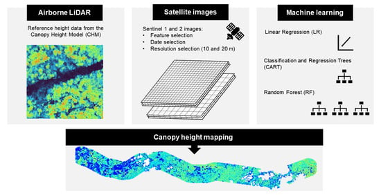
Canopy Height Mapping by Sentinel 1 and 2 Satellite Images, Airborne LiDAR Data, and Machine Learning

Abstract

Continuous mapping of vegetation height is critical for many forestry applications, such as planning vegetation management in power transmission line right-of-way. Satellite images from different sensors, including SAR (Synthetic Aperture Radar) from Sentinel 1 (S1) and multispectral from Sentinel 2 (S2), can be used for producing high-resolution vegetation height maps at a broad scale. The main objective of this study is to assess the potential of S1 and S2 satellite data, both in a single and a multisensor approach, for modeling canopy height in a transmission line right-of-way located in the Atlantic Forest of Paraná, Brazil. For integrating S1 and S2 data, we used three machine learning algorithms (LR: Linear Regression, CART: Classification and Regression Trees, and RF: Random Forest) and airborne LiDAR (Light Detection and Ranging) measurements as the reference height. The best models were obtained using the RF algorithm and 20 m resolution features from only S2 data (cross-validated RMSE of 4.92 m and R² of 0.58) or multisensor data (cross-validated RMSE of 4.86 m and R² of 0.60). Although the multisensor model presented the best performance, it was not statistically different from the single-S2 model. Thus, the use of only S2 to estimate canopy height has practical advantages, as it reduces the need to process SAR images and the uncertainties due to S1 noise or differences between the acquisition dates of S2 and S1.

1. Introduction

Mapping and monitoring forest structure variables, like canopy height, is crucial for several applications, such as assessment of ecosystem services [1], carbon stock quantification [2], wildlife management [3], and fire modeling [4]. Since vegetation height is affected by species composition, climate, and site quality, its measurement serves as an important ecological indicator and can be used to estimate stand age, successional stages, primary productivity, aboveground biomass, and biodiversity [5]. In addition, understanding the spatial and temporal variation of canopy height becomes an essential routine for projects that require constant vegetation management, such as in transmission line right-of-way. In these areas, trees that are very tall or close to transmission lines often need to be removed, as they pose a potential risk of accidents, interruption of power transmission service, as well as damage to the power system [6].

However, obtaining vegetation height measurements over large areas through field inventories is a difficult, expensive, time-consuming, and often dangerous activity, especially in forests with complex structure. Therefore, in situ measurements generally result in a limited number of sample plots, discontinued in time. To overcome these limitations, it is important to investigate alternative sources of vegetation structure data, such as remote sensing [7]. Active and passive remote sensing technologies enable monitoring on a larger scale, from the local scale for airborne sensors to the global scale for orbital sensors.

Among the various remote sensing options, active airborne LiDAR (Light Detection and Ranging) are recognized for providing high-precision height measurements [8]. Nevertheless, LiDAR is still an expensive technology, and its measurements are generally sparse in time and space, not covering very large areas. Though, airborne LiDAR data can be used in integration with freely available satellite remote sensing data, allowing the extrapolation of its high-precision height measurements into low-cost large-scale maps [5,9,10,11].

This strategy can be achieved through the application of machine learning techniques, which consists of learning a predictive model from satellite image features and known reference height values. Such height reference can be obtained by airborne LiDAR, which has proven to be a good substitute for field data. From the fitted predictive model and the remote sensing features used to adjust it, it is possible to estimate the vegetation height for unknown cases. Machine learning algorithms, such as Linear Regression (LR), Classification And Regression Trees (CART), and Random Forest (RF), have been effectively used in many remote sensing forestry applications [12,13].

Passive optical sensors aboard satellites such as Landsat constellation and Sentinel 2 (S2) capture spectral information related to vegetation structure and can be used to estimate height [9,14]. For example, several studies have used data from the Landsat satellite series to obtain vegetation height maps at a spatial resolution of 30 m [15,16,17]. Zhang et al. [17] mapped forest height at 30 m resolution by exploring the relationship between leaf area index (LAI) and canopy height from ICESat GLAS (Geoscience Laser Altimeter System on the Ice, Cloud, and Land Elevation Satellite), an orbital LiDAR. They first estimated LAI from Landsat data and then calibrated it with GLAS height for producing a height map with a 35% relative RMSE (Root Mean Square Error). Another example of a canopy height map from Landsat images is the one generated by Hansen et al. [15] in Sub-Saharan Africa.

Sentinel 2 satellites, from the European Space Agency’s (ESA) Copernicus program, carry a Multispectral Instrument (MSI) that, compared to the Landsat mission, is superior in spatial, temporal, and spectral resolution. However, few studies have explored the capabilities of S2 images to map vegetation height, especially in complex forests [10]. Some studies that compared the use of S2 and Landsat images to estimate forest structural properties [18,19,20] found that the S2 data performed slightly better than Landsat data. Although previous studies indicate the potential of multispectral images in predicting vegetation height, their use in complex vegetation, such as tropical and subtropical forests, can be a challenging task. This is mainly due to the frequent signal saturation in dense and high vegetation and the interference of clouds in the images, making it difficult or preventing obtaining optical data during the rainy season.

SAR (Synthetic Aperture Radar), an active remote sensing technology, overcome cloud cover problems, being a potential source of data for estimating vegetation height along different periods of the year. SAR images can be acquired in different microwave wavelengths, such as X-band, C-band, L-band, and P-band. Sentinel 1 (S1) satellites have been providing SAR data in the C-band (wavelength of 5.6 cm). SAR backscatter could be indirectly related to vegetation attributes, such as biomass [21,22]. For instance, airborne P-band SAR data have been successfully applied to biomass estimation across tropical and temperate forests [23,24,25].

Moreover, a promising alternative to improve vegetation height estimates is to integrate multisensor data from passive and active systems [26], like multispectral data from S2 and SAR data from S1. For instance, Moghaddam et al. [27] found that combining multispectral (Landsat) and SAR data was more accurate in predicting forest structure measurements than any single sensor alone. So far, only a few studies have explored the effectiveness of S1 and S2 data synergy for canopy height mapping [26,28,29], even less in tropical or subtropical ecosystems [14].

The main objective of this study is to evaluate the predictive potential of data from Sentinel 1 (S1) and Sentinel 2 (S2) satellites, used alone and in synergy, for mapping the vegetation height in the right-of-way of a transmission line located in the Atlantic Forest of Paraná, Brazil. For this, we used a machine learning approach in which three algorithms were tested (LR, CART, and RF) to combine satellite images from S1 and/or S2 with airborne LiDAR data as the reference height and generate high resolution (10 or 20 m) vegetation height maps.

As specific objectives, we aim to:

• Evaluate the relationship between the vegetation height measured by LiDAR and S1 and S2 features, in two spatial resolutions (10 and 20 m) and different periods of the year.
• Define the best approach to modeling the vegetation height, in order to evaluate the best set of S1 and S2 features and their spatial resolution, the proper time of year, and the most suitable machine learning algorithms (LR, CART, or RF).
• To analyze the generalization ability of a model trained with orbital data from a given date to estimate height based on data from other periods of the year.

2. Materials and Methods

2.1. Study Area and Datasets

The study area comprises the right-of-way of a power transmission line located in the state of Paraná-Brazil. The transmission line operates with a voltage of 138 kV in single circuit and is 52 km long, intersecting the municipalities of Campina Grande do Sul, Bocaiúva do Sul, and Tunas do Paraná. The natural vegetation that occurs in the region is composed of Mixed Ombrophilous Forest and Dense Ombrophilous Forest of the Brazilian Atlantic Forest biome. There are different stages of natural regeneration arising from cutting around the transmission line.

The remote sensing data used in this study consist of airborne LiDAR data, obtained for a buffer area of about 30 m on each side of the transmission line, and images from Sentinel 1 and Sentinel 2 satellites, obtained for a buffer area of 2 km on each side of the transmission line (Figure 1).

The airborne LiDAR data were collected on 22 October 2021, by a Leica/Hexagon ALS50-II system, which emits/receives laser beams at a wavelength of 1064 nm and an operating frequency of up to 150 kHz. The LiDAR data produced is of the discrete-return type, with a small footprint and an average density of 10 points/m². In addition to the LiDAR point cloud, the Digital Surface Model (DSM) and Digital Terrain Model (DTM) were also provided, at a spatial resolution of 0.5 m. From these models, we calculated the Canopy Height Model (CHM = DSM − DTM) to obtain the vegetation height used as a reference in the modeling approach. For this purpose, the 0.5 m CHM was averaged for 10 m and 20 m resolutions to match the spatial resolution of Sentinel images.

S2 satellite images for the year 2021 were downloaded from the European Space Agency’s (ESA) Copernicus Hub. For the same year, S1 with VV and VH polarization were downloaded from Google Earth Engine (GEE) using the Copernicus S1_GRD collections (IW instrument mode). GEE collection includes a set of preprocessing requirements such as GRD border noise removal, thermal noise removal, radiometric calibration, and terrain correction. More information is available at https://developers.google.com/earth-engine/guides/sentinel1 (accessed date: 10 December 2021).

A total of 26 dates for S1 images (from 10 January 2021 to 18 November 2021) and 40 dates for S2 images (from 9 January 2021 to 5 December 2021) were obtained. In order to compare the Sentinel images from multiple dates with the LiDAR data collected from just one date (22 October 2021), we assumed that the vegetation height exhibits little or no variation over a one-year period for the study area.

S1 images were originally provided at 10 m spatial resolution but were also resampled to 20 m resolution, in order to assess the effect of both resolutions on height estimation. Four indices were also calculated from the backscattering coefficients [30]:

• sum = VV + VH
• ratio = VV/VH
• Normalized Difference Index or NDI = (VV − VH)/(VV + VH)
• Radar Vegetation Index or RVI = 4×VH/(VV+VH)

Thus, a total of six S1 features were evaluated, including the VV and VH backscattering coefficients and derived indices, both for 10 m and 20 m resolution.

The S2 data used in this study consist of atmospherically corrected surface reflectance images from the Level-2A product. For each date, the two S2 scenes covering the study area were mosaicked by calculating the average for the overlapping areas. A masking of cloud and cloud shadow was applied to all the S2 images according to the information provided by the quality assessment band. We then used 10 S2 reflectance bands, of which four were obtained at 10 m resolution and six at 20 m resolution (

Table 1. Description of Sentinel 2 (S2) reflectance bands. NIR = Near Infrared, SWIR = Short Wave Infrared.

S2 Band	Description	Central Wavelength	Resolution
B02	Blue	490 nm	10 m (original) and 20 m (resampled)
B03	Green	560 nm	10 m (original) and 20 m (resampled)
B04	Red	665 nm	10 m (original) and 20 m (resampled)
B05	Red Edge 1	705 nm	20 m (original)
B06	Red Edge 2	740 nm	20 m (original)
B07	Red Edge 3	783 nm	20 m (original)
B08	NIR 1	842 nm	10 m (original) and 20 m (resampled)
B8A	NIR 2	865 nm	20 m (original)
B11	SWIR 1	1610 nm	20 m (original)
B12	SWIR 2	2190 nm	20 m (original)

). The four 10 m resolution bands were also resampled to 20 m resolution.

In addition to the surface reflectance, we also calculated 12 vegetation indices from S2 data, of which 4 were obtained only for the resolution of 10 m (

Table 2. Description of Sentinel 2 (S2) vegetation indices.

Vegetation Index	Formula	Resolution
Simple Ratio (SR)	SR = B08/B04	10 and 20 m
Normalized Difference Vegetation Index (NDVI)	NDVI = (B08 − B04)/(B08 + B04)	10 and 20 m
Green Normalized Difference Vegetation Index (GNDVI)	GNDVI = (B08 − B03)/(B08 + B03)	10 and 20 m
Vegetation Index green (VIgreen)	VIgreen = (B03 − B04)/(B03 + B04)	10 and 20 m
Red Edge Normalized Difference Vegetation Index (RENDVI)	RENDVI = (B07 − B04)/(B07 + B04)	20 m
Red Edge Simple Ratio (SRRE)	SRRE = B05/B04	20 m
Red edge Ratio Index 1 (RRI1)	RRI1 = B8A/B05	20 m
Inverted Red Edge Chlorophyll Index (IRECI)	IRECI = (B07−B04)/(B05/B06)	20 m
Moisture Stress Index (MSI)	MSI = B11/B8A	20 m
Normalized Difference Infrared Index (NDII)	NDII = (B8A − B11)/(B8A + B11)	20 m
Normalized Burn Ratio (NBR)	NBR = (B8A − B12)/(B8A + B12)	20 m
Specific Leaf Area Vegetation Index (SLAVI)	SLAVI = B8A/(B05 + B12)	20 m

). Thus, we evaluated a total of 8 S2 features with 10 m resolution and 22 S2 features with 20 m resolution, including both reflectance bands and vegetation indices.

To define the training samples for developing the height models, a stratified random sampling approach was used in order to guarantee a greater representation of different vegetation height ranges. For this, the 10 m CHM was divided into five strata of height: (1) 0–5 m, (2) 5–10 m, (3) 10–15 m, (4) 15–20 m, and (5) >20 m. Then, 20 samples were randomly distributed for each stratum. The center points of the resulting 100 training samples were used to select the corresponding pixels from the LiDAR height and Sentinel images. Thus, the vegetation height from LiDAR was considered as the dependent variable, while S1 and/or S2 features were considered as potential predictors for the machine learning models. Training samples (n = 100) were also used to evaluate the relationship between S1/S2 features and the LiDAR-based height, from which we calculated the Pearson’s correlation coefficient for each date, considering the resolutions of 10 m and 20 m. As some S2 images had many pixels without data due to the presence of clouds, we only considered the dates when at least 85% of the data were available.

Another 28 samples were randomly distributed in the study area (Figure 1) to test the ability of the best models to make generalizations based on Sentinel images obtained at different dates than those used for training the models. The mean LiDAR-based height and standard deviation of the 100 training samples are 12.47 m ± 8.21 m for the 10 m resolution CHM and 11.45 m ± 6.98 m for the 20 m resolution CHM. For the 28 test samples, the vegetation height is 10.80 m ± 5.74 m for the 10 m resolution CHM and 11.08 m ± 5.12 m for the 20 m resolution CHM.

2.2. Vegetation Height Modeling and Mapping

Figure 2 presents the methodological approach for modeling and mapping vegetation height based on S1 and/or S2 data, airborne LiDAR data, and machine learning models.

First, from the analysis of Pearson’s correlation coefficient for all available dates, we applied a feature selection strategy in order to identify and remove highly correlated S1 and S2 features, reducing the information redundancy to be introduced as input variables of the height models. Sentinel features in which the absolute correlation value with other features was greater than or equal to 0.95 in at least 50% of the evaluated dates were eliminated.

For training the height models, we considered the data from the 100 training samples, in which the LiDAR height values were taken as a reference, using both the 10 m and the 20 m resolution, and the selected S1/S2 features were taken as the predictor variables, also in both resolutions and divided into different datasets according to the source of the satellite data: (1) only S1, (2) only S2, (3) and the multisensor integration of S1 and S2 features. Furthermore, to define the best set of features for each data source, they were further subdivided into three subsets: (1) “raw”, which considers only the original data of each source, namely, the backscattering coefficients for the S1 data (VV and VH), the reflectance bands for the S2 data, and both for the multisensor data; (2) “ind”, which use only indices calculated from the original data of each source; and (3) “all”, which include all features selected for each data source.

To test the influence of the acquisition date of Sentinel images, we considered, for all datasets, data from two periods: images from May (May 22 for S1 and May 19 for S2) to represent the first semester and images from October (Oct 25 for S1 and Oct 26 for S2) to represent the second half. These dates were chosen because they presented few or no clouds in the S2 images and close acquisition dates between S1 and S2. Furthermore, for October, the dates closest to the acquisition of airborne LiDAR data were selected. In addition, for models with only one data source (S1 or S2), we also considered a date with high correlation between Sentinel features and LiDAR height (Sep 07 for S1 and Nov 30 for S2).

Three different machine learning algorithms were tested: LR (Multiple Linear Regression), CART (Classification and Regression Trees), and RF (Random Forest). LR is based on linear relationships between response and predictors and, due to its easy interpretation, is very popular in remote sensing applications. However, LR is a parametric model, requiring the assumptions of residual normality, homoscedasticity, and independence. Furthermore, it does not work properly with a large number of predictors and with non-linear relationships [31]. Non-parametric approaches, such as CART and RF, have the advantage of not making assumptions about the distribution of the data. CART works by recursively partitioning the data, resulting in a structure commonly known as a decision tree. RF is an ensemble model that combines predictions of multiple CART using a randomly selected subset of training samples and features. RF is recognized for its promising predictive capabilities for high-dimensional datasets and lower sensitivity to multicollinearity, data noise, outliers, and overfitting [12].

All modeling steps were developed in the R environment, using the caret package [32]. Considering the combinations of the two spatial resolutions (10 m and 20 m), three data sources (S1, S2, and S1_S2), three subsets of Sentinel features (“raw”, “ind”, and “all”), three algorithms (LR, CART, and RF), and the different image dates, a total of 144 models were tested, being 54 S1 models, 54 S2 models, and 36 S1_S2 models.

To define the best model from the 100 samples, a 10-fold cross-validation strategy was used, by calculating the following performance metrics: MAE (Mean Absolute Error), RMSE (Root Mean Square Error), and R² (coefficient of determination). Then, the best models for each data source were selected to be applied to the vegetation height mapping for the entire study area. To verify the ability to generalize the best models in an independent sample and other acquisition dates of the Sentinel images, we also proceeded with the calculation of the performance metrics (MAE, RMSE, and R²) for the test sample (n = 28).

3. Results

3.1. Relationship between LiDAR Height and Sentinel Features

The Sentinel 1 features obtained for the 100 training samples did not show a marked seasonal trend in the different acquisition dates, although they presented a high variation of values within the same image. The correlation values between the LiDAR height and the VV, VH, and sum features remained around 0.3 for all analyzed periods (Figure 3). These S1 features presented the highest correlation with LiDAR height (Figure 4), with values varying from 0.22 to 0.43 for VV, 0.21 to 0.42 for VH, and 0.28 to 0.45 for sum, when considering the 10 m resolution. For the 20 m resolution, the correlation values were slightly lower, in which the highest value reached was 0.37 for the S1 feature sum. The highest correlation values for these S1 features were observed for the date 07 September 2021.

The ratio index also showed some significant correlation values in relation to vegetation height (up to 0.35 for 10 m resolution and 0.28 for 20 m resolution). However, for some periods of the year, the correlation with this feature was not significant, which may be associated with the observation of greater noise in its values. The same was observed for the NDI and RVI indices, but with even lower correlation values, up to 0.29 for 10 m resolution and 0.26 for 20 m resolution. However, the NDI and RVI indices were eliminated in the feature selection step, as they were highly correlated with the ratio index. The sum index also showed a high correlation with the VV and VH polarizations, been eliminated when the “all” subset was considered. Thus, the S1 features considered for the modeling process were VV and VH for the “raw” subset, sum and ratio for the “ind” subset, and VV, VH, and ratio for the “all” subset.

The S2 features presented, in general, higher correlation with the vegetation height (values up to 0.69) than the S1 features. However, these values showed seasonality throughout the year, mainly for bands B06, B07, B08, and B8A (Figure 5) and vegetation indices (Figure 6). Overall, the months of May and June were the ones with the lowest correlation, while October, November, and December presented the highest correlation.

For the features that were calculated for both the 10 m and the 20 m resolution, little difference was observed in the correlation values between the two resolutions. However, the highest correlations were observed for features with 20 m, with mean values over the year of around 0.4 for features VIgreen (0.24–0.66), SLAVI (0.22–0.69), NBR (0.25–0.61), and B04 (0.21–0.54) (Figure 7).

In the feature selection step, among the 10 m resolution features, the GNDVI index was eliminated because it was highly correlated with the NDVI. For the 20 m resolution, we eliminated the bands B06, B08, and B8A, as they were correlated with band B07; the B11 band, due to its high correlation with the B12 band; the GNDVI and RENDVI indices, due to their correlation with the NDVI; and the NBR and MSI indices, due to their correlation with the NDII. Thus, a total of seven 10 m S2 features (B02, B03, B04, B08, SR, NDVI, and VIgreen) and 14 20 m S2 features (B02, B03, B04, B05, B07, B12, SR, SRRE, NDVI, VIgreen, RRI1, IRECI, NDII, and SLAVI) were left for modeling.

3.2. Vegetation Height Estimation Based on Sentinel 1 SAR Data

The performance of all vegetation height models based on S1 data is summarized in

Table 3. Performance metrics (MAE, RMSE, and R² calculated by cross-validation on the training sample) of vegetation height models based on Sentinel 1 (S1) data.

Algorithm	Features (*)	Resolution	Date	MAE	RMSE	R2
LR	raw (2)	10 m	May 22	6.13	7.65	0.16
	ind (2)	10 m	May 22	6.10	7.62	0.16
	all (3)	10 m	May 22	6.19	7.69	0.15
	raw (2)	10 m	Sep 07	5.77	7.16	0.28
	ind (2)	10 m	Sep 07	5.73	7.13	0.29
	all (3)	10 m	Sep 07	5.76	7.15	0.29
	raw (2)	10 m	Oct 25	5.95	7.38	0.20
	ind (2)	10 m	Oct 25	6.00	7.40	0.20
	all (3)	10 m	Oct 25	5.97	7.39	0.20
	raw (2)	20 m	May 22	5.33	6.55	0.12
	ind (2)	20 m	May 22	5.31	6.54	0.12
	all (3)	20 m	May 22	5.37	6.61	0.10
	raw (2)	20 m	Sep 07	5.12	6.30	0.20
	ind (2)	20 m	Sep 07	5.08	6.27	0.20
	all (3)	20 m	Sep 07	4.97	6.19	0.24
	raw (2)	20 m	Oct 25	5.14	6.32	0.20
	ind (2)	20 m	Oct 25	5.19	6.33	0.19
	all (3)	20 m	Oct 25	5.10	6.42	0.15
CART	raw	10 m	May 22	6.80	8.37	0.23
	ind	10 m	May 22	6.35	7.81	0.17
	all	10 m	May 22	7.36	9.07	0.21
	raw (2)	10 m	Sep 07	5.52	7.10	0.30
	ind (2)	10 m	Sep 07	5.69	7.36	0.34
	all (3)	10 m	Sep 07	5.64	7.11	0.32
	raw (2)	10 m	Oct 25	6.70	8.52	0.12
	ind (2)	10 m	Oct 25	6.55	8.39	0.18
	all (3)	10 m	Oct 25	6.57	8.54	0.11
	raw (2)	20 m	May 22	5.99	7.61	0.06
	ind (2)	20 m	May 22	6.05	7.37	0.06
	all (3)	20 m	May 22	6.13	7.70	0.05
	raw (2)	20 m	Sep 07	5.24	6.64	0.30
	ind (2)	20 m	Sep 07	5.17	6.59	0.26
	all (3)	20 m	Sep 07	5.27	6.65	0.30
	raw (2)	20 m	Oct 25	5.40	6.95	0.14
	ind (2)	20 m	Oct 25	5.73	7.29	0.15
	all (3)	20 m	Oct 25	5.79	7.29	0.13
RF	raw	10 m	May 22	6.52	8.17	0.17
	ind	10 m	May 22	6.39	7.74	0.16
	all	10 m	May 22	6.58	8.06	0.13
	raw (2)	10 m	Sep 07	5.81	7.44	0.25
	ind (2)	10 m	Sep 07	5.93	7.47	0.30
	all (3)	10 m	Sep 07	5.84	7.44	0.27
	raw (2)	10 m	Oct 25	6.52	8.16	0.13
	ind (2)	10 m	Oct 25	6.33	8.26	0.11
	all (3)	10 m	Oct 25	6.29	8.05	0.14
	raw (2)	20 m	May 22	6.21	7.58	0.04
	ind (2)	20 m	May 22	5.84	7.27	0.04
	all (3)	20 m	May 22	6.01	7.36	0.02
	raw (2)	20 m	Sep 07	5.27	6.79	0.27
	ind (2)	20 m	Sep 07	5.18	6.66	0.23
	all (3)	20 m	Sep 07	5.22	6.73	0.27
	raw (2)	20 m	Oct 25	5.44	6.70	0.15
	ind (2)	20 m	Oct 25	5.46	6.85	0.16
	all (3)	20 m	Oct 25	5.42	6.80	0.15

* The number of features is shown in parentheses.

. From the results of the performance metrics (MAE, RMSE, and R²), it was observed that the S1 models showed low performance in the estimation of vegetation height, with MAE ranging between 4.97–7.36 m, RMSE between 6.19-9.07 m, and R² between 0.02–0.34.

Models based on S1 features with a resolution of 20 m presented lower error values (MAE and RMSE) than models with 10 m features, especially those based on images from 7 September 2021 (date of highest correlation between LiDAR height and S1 features). However, the highest R² was reached on the same date but with 10 m resolution features. The combination of resolution and date that gave the worst result was obtained with the 20 m resolution models for the date of 22 May 2021.

Thus, the date and the spatial resolution of the S1 data were the factors that produced the greatest effect on the performance of models, with the machine learning algorithm and the subset of features having results varying according to these factors. For example, the model based on the LR algorithm, the subset of “all” features (VV, VH, and ratio) with 20 m resolution, and the date of September 7 had the lowest error among all models (MAE of 4.97 m and RMSE of 6.19 m). Among the models that used date from 25 October, the one with the lowest error (MAE of 5.14 m and RMSE of 6.32 m) was also based on the LR algorithm, but with the “raw” subset (VV and VH) with 20 m resolution. And the highest R² (0.34) was obtained for the date of Sep 7 with the CART algorithm, but using the subset of “ind” features (sum and ratio) with 10 m resolution. However, this model presented a higher error (MAE of 5.69 m and RMSE of 7.36 m) than that obtained with the LR algorithm.

3.3. Vegetation Height Estimation Based on Sentinel 2 Multispectral Data

Table 4. Performance metrics (MAE, RMSE, and R² calculated by cross-validation on the training sample) of vegetation height models based on Sentinel 2 (S2) data.

Algorithm	Features (*)	Resolution	Date	MAE	RMSE	R2
LR	raw (4)	10 m	May 19	6.73	8.24	0.15
	ind (3)	10 m	May 19	7.40	10.37	0.14
	all (7)	10 m	May 19	6.81	8.81	0.20
	raw (4)	10 m	Oct 26	5.55	7.08	0.36
	ind (3)	10 m	Oct 26	5.95	7.37	0.35
	all (7)	10 m	Oct 26	5.43	6.68	0.38
	raw (4)	10 m	Nov 30	5.46	6.71	0.33
	ind (3)	10 m	Nov 30	5.60	6.86	0.29
	all (7)	10 m	Nov 30	5.68	7.31	0.34
	raw (6)	20 m	May 19	5.02	6.31	0.26
	ind (8)	20 m	May 19	5.90	8.84	0.27
	all (14)	20 m	May 19	5.35	7.08	0.31
	raw (6)	20 m	Oct 26	4.35	5.61	0.45
	ind (8)	20 m	Oct 26	4.62	6.18	0.43
	all (14)	20 m	Oct 26	4.02	5.15	0.56
	raw (6)	20 m	Nov 30	4.50	5.85	0.37
	ind (8)	20 m	Nov 30	4.57	6.09	0.47
	all (14)	20 m	Nov 30	3.92	4.91	0.54
CART	raw (4)	10 m	May 19	7.52	8.79	0.08
	ind (3)	10 m	May 19	6.82	8.33	0.13
	all (7)	10 m	May 19	7.34	8.94	0.09
	raw (4)	10 m	Oct 26	6.59	7.94	0.17
	ind (3)	10 m	Oct 26	5.62	7.17	0.31
	all (7)	10 m	Oct 26	5.93	7.60	0.25
	raw (4)	10 m	Nov 30	6.04	7.28	0.29
	ind (3)	10 m	Nov 30	6.04	7.45	0.28
	all (7)	10 m	Nov 30	6.17	7.79	0.25
	raw (6)	20 m	May 19	5.73	7.03	0.23
	ind (8)	20 m	May 19	5.83	7.07	0.15
	all (14)	20 m	May 19	5.67	6.97	0.16
	raw (6)	20 m	Oct 26	4.56	5.78	0.43
	ind (8)	20 m	Oct 26	4.93	6.34	0.36
	all (14)	20 m	Oct 26	5.01	6.22	0.38
	raw (6)	20 m	Nov 30	4.41	5.38	0.46
	ind (8)	20 m	Nov 30	4.68	5.60	0.38
	all (14)	20 m	Nov 30	4.82	5.60	0.40
RF	raw (4)	10 m	May 19	6.91	8.31	0.14
	ind (3)	10 m	May 19	6.78	8.19	0.14
	all (7)	10 m	May 19	6.69	8.05	0.17
	raw (4)	10 m	Oct 26	6.07	7.44	0.24
	ind (3)	10 m	Oct 26	6.00	7.32	0.25
	all (7)	10 m	Oct 26	5.71	6.98	0.33
	raw (4)	10 m	Nov 30	5.87	6.92	0.33
	ind (3)	10 m	Nov 30	6.16	7.62	0.22
	all (7)	10 m	Nov 30	5.64	6.76	0.35
	raw (6)	20 m	May 19	5.17	6.31	0.23
	ind (8)	20 m	May 19	4.95	6.06	0.28
	all (14)	20 m	May 19	4.98	6.08	0.25
	raw (6)	20 m	Oct 26	3.88	4.92	0.58
	ind (8)	20 m	Oct 26	4.05	5.06	0.50
	all (14)	20 m	Oct 26	3.95	4.90	0.55
	raw (6)	20 m	Nov 30	3.92	4.79	0.55
	ind (8)	20 m	Nov 30	4.00	4.94	0.51
	all (14)	20 m	Nov 30	3.97	4.84	0.53

* The number of features is shown in parentheses.

shows the results of the performance metrics (MAE, RMSE, and R²) for the S2 models. In general, S2 models showed better performance than S1 models, with MAE ranging between 3.88–7.52 m, RMSE between 4.79–10.37 m, and R² between 0.08–0.58. However, the S2 models showed great variation in performance depending on the date of acquisition, with the date of 19 May showing the worst results and the dates of 26 October and 30 November, the best.

In addition to the date, models that used the 20 m resolution data also performed better than the models with 10 m resolution. For example, the S2 model with the lowest MAE (3.88) and highest R² (0.58) was the one that used the RF algorithm, “raw” dataset (only reflectance bands) in the date 26 October, and 20 m resolution data. The model with the same characteristics, except for the 10 m resolution, had an MAE of 6.07 m and an R² of 0.24.

Regarding the algorithm, in general, the CART had a lower performance than the RF and LR. Considering the different subsets of features, it was observed that for most models, the use of only reflectance bands (“raw” dataset) performed as well or better than the use of vegetation indices (“ind”) or the complete feature set (“all”), even with a smaller number of features.

3.4. Vegetation Height Estimation Based on the Integration of Sentinel 1 SAR Data and Sentinel 2 Multispectral Data

Table 5. Performance metrics (MAE, RMSE, and R² calculated by cross-validation on the training sample) of vegetation height models based on both Sentinel 1 and 2 (S1_S2) data.

Algorithm	Features (*)	Resolution	Date	MAE	RMSE	R2
LR	raw (6)	10 m	May 22 (S1) and 19 (S2)	6.55	8.15	0.17
	ind (5)	10 m	May 22 (S1) and 19 (S2)	7.22	10.24	0.15
	all (10)	10 m	May 22 (S1) and 19 (S2)	6.91	9.31	0.17
	raw (6)	10 m	Oct 25 (S1) and 26 (S2)	5.36	7.03	0.42
	ind (5)	10 m	Oct 25 (S1) and 26 (S2)	5.36	6.76	0.38
	all (10)	10 m	Oct 25 (S1) and 26 (S2)	5.03	6.17	0.45
	raw (8)	20 m	May 22 (S1) and 19 (S2)	5.15	6.49	0.25
	ind (10)	20 m	May 22 (S1) and 19 (S2)	5.78	8.56	0.24
	all (17)	20 m	May 22 (S1) and 19 (S2)	5.47	7.27	0.26
	raw (8)	20 m	Oct 25 (S1) and 26 (S2)	4.34	5.54	0.50
	ind (10)	20 m	Oct 25 (S1) and 26 (S2)	4.22	5.76	0.48
	all (17)	20 m	Oct 25 (S1) and 26 (S2)	4.19	5.29	0.56
CART	raw (6)	10 m	May 22 (S1) and 19 (S2)	7.33	8.84	0.12
	ind (5)	10 m	May 22 (S1) and 19 (S2)	6.37	7.76	0.20
	all (10)	10 m	May 22 (S1) and 19 (S2)	7.38	9.13	0.14
	raw (6)	10 m	Oct 25 (S1) and 26 (S2)	6.44	7.85	0.25
	ind (5)	10 m	Oct 25 (S1) and 26 (S2)	5.73	7.35	0.29
	all (10)	10 m	Oct 25 (S1) and 26 (S2)	5.73	7.37	0.33
	raw (8)	20 m	May 22 (S1) and 19 (S2)	5.38	6.70	0.21
	ind (10)	20 m	May 22 (S1) and 19 (S2)	5.55	6.74	0.17
	all (17)	20 m	May 22 (S1) and 19 (S2)	5.25	6.58	0.22
	raw (8)	20 m	Oct 25 (S1) and 26 (S2)	4.20	5.28	0.50
	ind (10)	20 m	Oct 25 (S1) and 26 (S2)	4.89	6.22	0.38
	all (17)	20 m	Oct 25 (S1) and 26 (S2)	5.06	6.25	0.37
RF	raw (6)	10 m	May 22 (S1) and 19 (S2)	6.37	7.78	0.13
	ind (5)	10 m	May 22 (S1) and 19 (S2)	6.20	7.55	0.16
	all (10)	10 m	May 22 (S1) and 19 (S2)	6.35	7.71	0.15
	raw (6)	10 m	Oct 25 (S1) and 26 (S2)	5.80	7.22	0.28
	ind (5)	10 m	Oct 25 (S1) and 26 (S2)	5.09	6.38	0.45
	all (10)	10 m	Oct 25 (S1) and 26 (S2)	5.19	6.52	0.40
	raw (8)	20 m	May 22 (S1) and 19 (S2)	5.02	6.15	0.21
	ind (10)	20 m	May 22 (S1) and 19 (S2)	4.83	5.94	0.31
	all (17)	20 m	May 22 (S1) and 19 (S2)	4.90	5.97	0.24
	raw (8)	20 m	Oct 25 (S1) and 26 (S2)	3.62	4.86	0.60
	ind (10)	20 m	Oct 25 (S1) and 26 (S2)	3.77	4.83	0.56
	all (17)	20 m	Oct 25 (S1) and 26 (S2)	3.67	4.71	0.59

* The number of features is shown in parentheses.

shows the performance of models based on multisensor data integration (S1 and S2), in which MAE values ranged from 3.62–7.38 m, RMSE from 4.71–10.24 m, and R² from 0.12–0.60. In general, the results of multisensor models were similar to the ones with only S2 data. Therefore, the performance of multisensor models was also affected by the date of acquisition, with models based on October data performing better than models from May.

In addition, similarly to what was observed for the S2 models, the best performance (lower MAE and RMSE and greater R²) of the multisensor data occurred with the use of features of 20 m resolution, especially those based on the RF algorithm and October date (MAE of 3.62–3.77 m, RMSE of 4.71–4.86 m and R² of 0.56–0.60). The subset of features used in these models did not produce significant variation in performance. However, the use of the “raw” subset proved to be more advantageous, as it produces the smallest MAE (3.62) and highest R² (0.60), in addition to requiring the least number of features. The CART algorithm also displayed a lower performance in comparison with the RF and LR, as noted for the S2-only models.

3.5. Generalization Ability of the Best Models

Based on the performance metrics of all the 144 evaluated models (Table 3, Table 4 and Table 5), we selected the best models for each data source: for S1, the model with the LR algorithm and “all” S1 features with 20 m resolution from Sep 07; for S2, the model with the RF algorithm and “raw” S2 features with 20 m resolution from Oct 26; and for multisensor, the model with the RF algorithm and “raw” S1 and S2 features with 20 m resolution from Oct 25/26. When comparing the three data sources, it is observed that the best results are obtained using S2 or S1_S2 data, with no significant difference in performance between the two. On the other hand, the model derived from the S1 SAR data presented significantly lower performance than the models with S2 or multisensor data, especially with respect to R² (Figure 8).

When considering the validation of the best models in the test sample (n = 28), it was found that the error (MAE of 4.29 m for S1, 3.88 m for S2, and 3.69 m for S1_S2; and RMSE of 5.38 m for S1, 4.78 m for S2, and 4.48 m for S1_S2) remained very similar to that calculated in the training sample, showing good generalization when used in independent samples. In relative terms, considering the average height of the samples of about 11 m, the best model (S1_S2) achieved a relative MAE of 32% for the training sample and 33% for the test sample, and a relative RMSE of 42% for the training sample and 40% for the test sample. The R² calculated in the test sample (0.00 for S1, 0.18 for S2, and 0.25 for S1_S2) showed lower values than the training sample, which can be explained by the influence of the sample size on this metric, which becomes more sensitive to outliers (Figure 9).

The temporal variation of performance metrics in the test sample was also analyzed to assess whether the best models, calibrated with data from specific dates, can be extrapolated to predict vegetation height based on images from other Sentinel acquisition dates. Thus, Figure 10 shows the variation of the test- RMSE and R² of the best multisensor models (S1_S2) calibrated with different data subsets (“raw”, “ind”, and “all”) in two periods (May and October), extrapolated to images from other dates of the year 2021. Overall, the lowest RMSE and highest R² values occur when models trained with October data are applied to images between August and November. The models trained with data from May showed lower RMSE for the period from January to July, despite having higher R² from September to November. The models based on the “raw” features of both periods showed the lowest error values throughout the year and the highest R² values (especially after August), when compared to the models based on the indices (“ind”) or all features (“all”). Thus, the “raw” models (both those based on S2 or multisensor data) are the ones with the best performance, but their ability to generalize to other images is restricted to the period between August and November.

Figure 11 presents the vegetation height maps derived from the best models of each data source (S1, S2, and S1_S2), all with 20 m spatial resolution. It is observed that the map derived only from the S1 data shows a topographic effect on the variation of height estimates. Therefore, the map that uses only S2 data can be chosen to avoid this type of noise. However, it is worth considering that maps that use S2 data (single-S2 or multisensor) will be influenced by clouds, and may not provide estimates in rainy seasons.

4. Discussion and Conclusions

The best models for the vegetation height estimation were obtained using S2 data or with the combination of S2 and S1 data, in both cases with images of 20 m resolution. Although the model based on the combination of S2 and S1 data presented the best performance (smallest error and highest R²), it was not statistically different from the model based only on S2 data, indicating that the information gained by adding S1 data was not significant. Moreover, the S1 data when used in combination with S2 data can add unwanted noises, such as noise remaining from data pre-processing (e.g., topographical effect) or due to the difference between the acquisition dates of the images, since the S1 and S2 images are not always available for close dates. Thus, the use of only S2 to estimate canopy height has practical advantages, as it reduces the need to process SAR images, as well as the uncertainties that it can add due to noise or differences in land cover between the acquisition dates of S2 and S1.

Our results are in agreement with those found by Hyde et al. [3] that compared the performance of LiDAR, multispectral (Landsat and Quickbird), and SAR data for estimating canopy height by linear regression models. They found that the addition of SAR and Quickbird data improved estimates only marginally than the use of single Landsat ETM+ or a combination of LiDAR and Landsat ETM+.

Furthermore, our results also show that models based only on S1 data presented the highest errors. The lower performance of the S1 data may be related to the low capacity of its C-band to penetrate the canopy of structurally complex forests [33]. Other SAR systems, such as X-band, can also have the same problem. For instance, Kugler et al. [34] assessed the TanDEM-X SAR data for height estimation in three different forest types (boreal, temperate, and tropical), finding less accurate results for the tropical forests. The use of P-band SAR has great potential to overcome these limitations in estimating structural attributes such as canopy height and aboveground biomass (AGB). The ESA’s BIOMASS, to be launched in 2023, will be the first P-band SAR mission in space. The main objectives of the BIOMASS mission are producing 200 m spatial resolution maps of both forest AGB and height and a 50 m spatial resolution map of forest disturbance. These maps are expected to be more accurate in complex ecosystems than those produced by SAR with shorter wavelengths, such as L, C, or X-band [35,36].

Regarding the S2 features that produced the best performance, we found that using only reflectance bands at 20 m resolution (“raw” subset) generally performs better than adding vegetation indices. The better performance of the 20 m bands is justified by the addition of important spectral regions to obtain structural information, such as the red edge and SWIR bands [20], that are not available in the 10 m resolution. However, the addition of vegetation indices proved to be redundant in relation to reflectance bands. Other studies also report that using directly the S2 bands was better or at least equivalent than using derived vegetation indices for retrieving forest structural information [19,20].

In addition, the vegetation indices also showed high seasonality, which produces models that are not generalizable for other periods of the year. The NIR (B08 and B8A) and red-edge bands closer to the NIR (B06 and B07) also showed high seasonality. As many vegetation indices are based on NIR bands, this seasonality ends up being accentuated by their use. Despite the high seasonality of these S2 features, the vegetation height is expected to vary little within a year, unless there is an abrupt change in land cover, such as clearcutting. Thus, such features produce differences in the modeling depending on the date of the image used, restricting possible applications that depend on continuous height estimates and their temporal analysis.

Although this temporal variation presents disadvantages for applications based on single images, it can be exploited to produce better models of canopy height on the annual scale. For instance, Trier et al. [9] used multitemporal data from Landsat and ALOS PALSAR satellites to produce a yearly estimate of vegetation height. They found that using all available Landsat acquisitions of the same area within one year reduced the estimation error variance, while the addition of SAR data from ALOS PALSAR produced only a small increase in the performance of the models. In this context, the authors consider that the use of repeated Landsat acquisitions during the same year makes it possible to find relationships between seasonal changes and vegetation height, since it can be assumed that tall vegetations, like forests, are better at preserving its greenness than low stature vegetation, such as grass and crops. In addition, the use of mosaics from images of different dates can reduce cloud interference. However, some applications require the production of estimates in a given time period, in which future studies could assess whether it is possible to improve estimates, mainly for rainy periods.

For future works, it would be interesting to have reference height data from LiDAR or field inventories for more than one date, preferably covering the dry and rainy seasons, to better investigate the effect of temporal variations on the performance of the models. In addition to exploring temporal variation, another alternative for improving the models would be to explore the spatial patterns of neighboring pixels, through textural metrics, which can add information like vegetation shadowing and roughness [37]. Another promising alternative for modeling continuous variables from remote sensing images is deep learning techniques [10], which, together with other machine learning approaches, can be tested in future studies to seek possible performance improvements.

Our best model showed a relative RMSE of around 40%, in agreement with other studies, such as [38] that showed a relative RMSE of 36.7% in boreal forests, and [17], whose relative RMSE was 35.2% in temperate forests, both using Landsat data. However, it is expected that height estimates in structurally complex vegetation, such as the one evaluated in our study, present greater error than those produced in more homogeneous vegetation. For example, Lang et al. [10], estimated vegetation height from S2 data for two landscapes: a complex tropical forest in Gabon and a vegetation with lower height and density in Switzerland. The resulting maps have an RMSE of 3.4 m in Switzerland and 5.6 m in Gabon. Moreover, our local model is more accurate than the global forest height map from Potapov et al. [16], which showed an RMSE of 9.07 m and R² of 0.61 when validated with airborne LiDAR for selected areas in the USA, Mexico, the Democratic Republic of the Congo, and Australia. Comparing the values from this global map with the airborne LiDAR data samples used in our study, we found an RMSE of 5.46 m and R² of 0.23 (Figure S1, in the supplementary material). Therefore, for our study area, this global model showed a tendency to overestimate values below 10 m and underestimate values greater than 10 m. However, it must be considered that the global map was developed for the year 2019 and the LiDAR data for our study area were obtained in 2021, which may cause some small differences in height between the two years.

The methodology used in this study integrates remote sensing and machine learning techniques, proving to be a powerful tool for continuous mapping of vegetation height on a large scale. Although future studies can be carried out to further improve the performance of our models, the height maps produced here can still be useful as low-cost prior information for various applications, such as forest monitoring, management, and planning. With regard to areas in the right-of-way of transmission lines, vegetation height maps can help to save on in-situ visit costs, for example, by eliminating from these visits the areas of low vegetation that potentially offer low risk for the maintenance of the transmission line.

References

1. Abelleira Martínez, O.J.; Fremier, A.K.; Günter, S.; Ramos Bendaña, Z.; Vierling, L.; Galbraith, S.M.; Bosque-Pérez, N.A.; Ordoñez, J.C. Scaling up Functional Traits for Ecosystem Services with Remote Sensing: Concepts and Methods. Ecol. Evol. 2016, 6, 4359–4371. [Google Scholar] [CrossRef] [PubMed]
2. Karna, Y.K.; Hussin, Y.A.; Gilani, H.; Bronsveld, M.C.; Murthy, M.S.R.; Qamer, F.M.; Karky, B.S.; Bhattarai, T.; Aigong, X.; Baniya, C.B. Integration of WorldView-2 and Airborne LiDAR Data for Tree Species Level Carbon Stock Mapping in Kayar Khola Watershed, Nepal. Int. J. Appl. Earth Obs. Geoinf. 2015, 38, 280–291. [Google Scholar] [CrossRef]
3. Hyde, P.; Dubayah, R.; Walker, W.; Blair, J.B.; Hofton, M.; Hunsaker, C. Mapping Forest Structure for Wildlife Habitat Analysis Using Multi-Sensor (LiDAR, SAR/InSAR, ETM+, Quickbird) Synergy. Remote Sens. Environ. 2006, 102, 63–73. [Google Scholar] [CrossRef]
4. Arroyo, L.A.; Pascual, C.; Manzanera, J.A. Fire Models and Methods to Map Fuel Types: The Role of Remote Sensing. For. Ecol. Manag. 2008, 256, 1239–1252. [Google Scholar] [CrossRef] [Green Version]
5. Stojanova, D.; Panov, P.; Gjorgjioski, V.; Kobler, A.; Džeroski, S. Estimating Vegetation Height and Canopy Cover from Remotely Sensed Data with Machine Learning. Ecol. Inform. 2010, 5, 256–266. [Google Scholar] [CrossRef]
6. Mills, S.J.; Gerardo Castro, M.P.; Li, Z.; Cai, J.; Hayward, R.; Mejias, L.; Walker, R.A. Evaluation of Aerial Remote Sensing Techniques for Vegetation Management in Power-Line Corridors. IEEE Trans. Geosci. Remote Sens. 2010, 48, 3379–3390. [Google Scholar] [CrossRef]
7. Wulder, M.A.; Seemann, D. Forest Inventory Height Update through the Integration of Lidar Data with Segmented Landsat Imagery. Can. J. Remote Sens. 2003, 29, 536–543. [Google Scholar] [CrossRef]
8. Lim, K.; Treitz, P.; Wulder, M.; St-Ongé, B.; Flood, M. LiDAR Remote Sensing of Forest Structure. Prog. Phys. Geogr. 2003, 27, 88–106. [Google Scholar] [CrossRef] [Green Version]
9. Trier, Ø.D.; Salberg, A.B.; Haarpaintner, J.; Aarsten, D.; Gobakken, T.; Næsset, E. Multi-Sensor Forest Vegetation Height Mapping Methods for Tanzania. Eur. J. Remote Sens. 2018, 51, 587–606. [Google Scholar] [CrossRef] [Green Version]
10. Lang, N.; Schindler, K.; Wegner, J.D. Country-Wide High-Resolution Vegetation Height Mapping with Sentinel-2. Remote Sens. Environ. 2019, 233, 111347. [Google Scholar] [CrossRef] [Green Version]
11. Hudak, A.T.; Lefsky, M.A.; Cohen, W.B.; Berterretche, M. Integration of Lidar and Landsat ETM+ Data for Estimating and Mapping Forest Canopy Height. Remote Sens. Environ. 2002, 82, 397–416. [Google Scholar] [CrossRef] [Green Version]
12. Belgiu, M.; Dragut, L. Random Forest in Remote Sensing: A Review of Applications and Future Directions. ISPRS J. Photogramm. Remote Sens. 2016, 114, 24–31. [Google Scholar] [CrossRef]
13. Maxwell, A.E.; Warner, T.A.; Fang, F. Implementation of Machine-Learning Classification in Remote Sensing: An Applied Review. Int. J. Remote Sens. 2018, 39, 2784–2817. [Google Scholar] [CrossRef] [Green Version]
14. Ghosh, S.M.; Behera, M.D.; Paramanik, S. Canopy Height Estimation Using Sentinel Series Images through Machine Learning Models in a Mangrove Forest. Remote Sens. 2020, 12, 1519. [Google Scholar] [CrossRef]
15. Hansen, M.C.; Potapov, P.V.; Goetz, S.J.; Turubanova, S.; Tyukavina, A.; Krylov, A.; Kommareddy, A.; Egorov, A. Mapping Tree Height Distributions in Sub-Saharan Africa Using Landsat 7 and 8 Data. Remote Sens. Environ. 2016, 185, 221–232. [Google Scholar] [CrossRef] [Green Version]
16. Potapov, P.; Li, X.; Hernandez-Serna, A.; Tyukavina, A.; Hansen, M.C.; Kommareddy, A.; Pickens, A.; Turubanova, S.; Tang, H.; Silva, C.E.; et al. Mapping Global Forest Canopy Height through Integration of GEDI and Landsat Data. Remote Sens. Environ. 2021, 253, 112165. [Google Scholar] [CrossRef]
17. Zhang, G.; Ganguly, S.; Nemani, R.R.; White, M.A.; Milesi, C.; Hashimoto, H.; Wang, W.; Saatchi, S.; Yu, Y.; Myneni, R.B. Estimation of Forest Aboveground Biomass in California Using Canopy Height and Leaf Area Index Estimated from Satellite Data. Remote Sens. Environ. 2014, 151, 44–56. [Google Scholar] [CrossRef]
18. Astola, H.; Häme, T.; Sirro, L.; Molinier, M.; Kilpi, J. Comparison of Sentinel-2 and Landsat 8 Imagery for Forest Variable Prediction in Boreal Region. Remote Sens. Environ. 2019, 223, 257–273. [Google Scholar] [CrossRef]
19. Korhonen, L.; Hadi; Packalen, P.; Rautiainen, M. Comparison of Sentinel-2 and Landsat 8 in the Estimation of Boreal Forest Canopy Cover and Leaf Area Index. Remote Sens. Environ. 2017, 195, 259–274. [Google Scholar] [CrossRef]
20. Chrysafis, I.; Mallinis, G.; Siachalou, S.; Patias, P. Assessing the Relationships between Growing Stock Volume and Sentinel-2 Imagery in a Mediterranean Forest Ecosystem. Remote Sens. Lett. 2017, 8, 508–517. [Google Scholar] [CrossRef]
21. Luckman, A.; Baker, J.; Kuplich, T.M.; Corina da Costa, F.Y.; Alejandro, C.F. A Study of the Relationship between Radar Backscatter and Regenerating Tropical Forest Biomass for Spaceborne SAR Instruments. Remote Sens. Environ. 1997, 60, 1–13. [Google Scholar] [CrossRef]
22. Bispo, P.d.C.; Rodríguez-Veiga, P.; Zimbres, B.; do Couto de Miranda, S.; Giusti Cezare, C.H.; Fleming, S.; Baldacchino, F.; Louis, V.; Rains, D.; Garcia, M.; et al. Woody Aboveground Biomass Mapping of the Brazilian Savanna with a Multi-Sensor and Machine Learning Approach. Remote Sens. 2020, 12, 2685. [Google Scholar] [CrossRef]
23. Santi, E.; Paloscia, S.; Pettinato, S.; Cuozzo, G.; Padovano, A.; Notarnicola, C.; Albinet, C. Machine-Learning Applications for the Retrieval of Forest Biomass from Airborne P-Band SAR Data. Remote Sens. 2020, 12, 804. [Google Scholar] [CrossRef] [Green Version]
24. Soja, M.J.; Quegan, S.; d’Alessandro, M.M.; Banda, F.; Scipal, K.; Tebaldini, S.; Ulander, L.M.H. Mapping Above-Ground Biomass in Tropical Forests with Ground-Cancelled P-Band SAR and Limited Reference Data. Remote Sens. Environ. 2021, 253, 112153. [Google Scholar] [CrossRef]
25. Schlund, M.; Davidson, M.W.J. Aboveground Forest Biomass Estimation Combining L- and P-Band SAR Acquisitions. Remote Sens. 2018, 10, 1151. [Google Scholar] [CrossRef] [Green Version]
26. Liu, Y.; Gong, W.; Xing, Y.; Hu, X.; Gong, J. Estimation of the Forest Stand Mean Height and Aboveground Biomass in Northeast China Using SAR Sentinel-1B, Multispectral Sentinel-2A, and DEM Imagery. ISPRS J. Photogramm. Remote Sens. 2019, 151, 277–289. [Google Scholar] [CrossRef]
27. Moghaddam, M.; Dungan, J.L.; Acker, S. Forest Variable Estimation from Fusion of SAR and Multispectral Optical Data. IEEE Trans. Geosci. Remote Sens. 2002, 40, 2176–2187. [Google Scholar] [CrossRef]
28. Morin, D.; Planells, M.; Baghdadi, N.; Bouvet, A.; Fayad, I.; Le Toan, T.; Mermoz, S.; Villard, L. Improving Heterogeneous Forest Height Maps by Integrating GEDI-Based Forest Height Information in a Multi-Sensor Mapping Process. Remote Sens. 2022, 14, 2079. [Google Scholar] [CrossRef]
29. Li, W.; Niu, Z.; Shang, R.; Qin, Y.; Wang, L.; Chen, H. High-Resolution Mapping of Forest Canopy Height Using Machine Learning by Coupling ICESat-2 LiDAR with Sentinel-1, Sentinel-2 and Landsat-8 Data. Int. J. Appl. Earth Obs. Geoinf. 2020, 92, 102163. [Google Scholar] [CrossRef]
30. Nasirzadehdizaji, R.; Sanli, F.B.; Abdikan, S.; Cakir, Z.; Sekertekin, A.; Ustuner, M. Sensitivity Analysis of Multi-Temporal Sentinel-1 SAR Parameters to Crop Height and Canopy Coverage. Appl. Sci. 2019, 9, 655. [Google Scholar] [CrossRef] [Green Version]
31. Osborne, J.; Waters, E. Four Assumptions of Multiple Regression That Researchers Should Always Test. Pract. Assess. Res. Eval. 2002, 8, 1. [Google Scholar]
32. Kuhn, M. Building Predictive Models in R Using the Caret Package. J. Stat. Softw. 2008, 28, 1–26. [Google Scholar] [CrossRef] [Green Version]
33. Pourshamsi, M.; Xia, J.; Yokoya, N.; Garcia, M.; Lavalle, M.; Pottier, E.; Balzter, H. Tropical Forest Canopy Height Estimation from Combined Polarimetric SAR and LiDAR Using Machine-Learning. ISPRS J. Photogramm. Remote Sens. 2021, 172, 79–94. [Google Scholar] [CrossRef]
34. Kugler, F.; Lee, S.K.; Hajnsek, I.; Papathanassiou, K.P. Forest Height Estimation by Means of Pol-InSAR Data Inversion: The Role of the Vertical Wavenumber. IEEE Trans. Geosci. Remote Sens. 2015, 53, 5294–5311. [Google Scholar] [CrossRef]
35. Fatoyinbo, T.; Armston, J.; Simard, M.; Saatchi, S.; Denbina, M.; Lavalle, M.; Hofton, M.; Tang, H.; Marselis, S.; Pinto, N.; et al. The NASA AfriSAR Campaign: Airborne SAR and Lidar Measurements of Tropical Forest Structure and Biomass in Support of Current and Future Space Missions. Remote Sens. Environ. 2021, 264, 112533. [Google Scholar] [CrossRef]
36. Banda, F.; Giudici, D.; Le Toan, T.; d’Alessandro, M.M.; Papathanassiou, K.; Quegan, S.; Riembauer, G.; Scipal, K.; Soja, M.; Tebaldini, S.; et al. The BIOMASS Level 2 Prototype Processor: Design and Experimental Results of above-Ground Biomass Estimation. Remote Sens. 2020, 12, 985. [Google Scholar] [CrossRef] [Green Version]
37. Wood, E.M.; Pidgeon, A.M.; Radeloff, V.C.; Keuler, N.S. Image Texture as a Remotely Sensed Measure of Vegetation Structure. Remote Sens. Environ. 2012, 121, 516–526. [Google Scholar] [CrossRef]
38. Hyyppä, J.; Hyyppä, H.; Inkinen, M.; Engdahl, M.; Linko, S.; Zhu, Y.H. Accuracy Comparison of Various Remote Sensing Data Sources in the Retrieval of Forest Stand Attributes. For. Ecol. Manag. 2000, 128, 109–120. [Google Scholar] [CrossRef]
Figure 1. (A) Study area, with the distribution of data and samples along the transmission line. (B) Zoom of the area with LiDAR data and examples of training and test samples. (C) Location of the state of Paraná in South America.
Remotesensing 14 04112 g001
Figure 2. Methodological flowchart for modeling and mapping the vegetation height of the study area.
Remotesensing 14 04112 g002
Figure 3. Correlation coefficient of LiDAR heigh against the 6 Sentinel 1 (S1) features, both for 10 m and 20 m resolution, for all available dates in 2021. Dates with significant correlation are represented in black.
Remotesensing 14 04112 g003
Figure 4. Relationship between the LiDAR height and the Sentinel 1 (S1) features that presented the highest correlation (for 10 m resolution), for the three dates used in the construction of the vegetation height models.
Remotesensing 14 04112 g004
Figure 5. Correlation coefficient of LiDAR heigh against the 10 Sentinel 2 (S2) bands, both for 10 m and 20 m resolution, for dates in 2021 with at least 85% of the samples without cloud. Dates with significant correlation are represented in black.
Remotesensing 14 04112 g005
Figure 6. Correlation coefficient of LiDAR heigh against the 12 Sentinel 2 (S2) vegetation indices, both for 10 m and 20 m resolution, for dates in 2021 with at least 85% of the samples without cloud. Dates with significant correlation are represented in black.
Remotesensing 14 04112 g006
Figure 7. Relationship between the LiDAR height and the Sentinel 2 (S2) features (VIgreen, SLAVI, NBR, and B04) that presented the highest correlation (for 20 m resolution), for the three dates used in the construction of the vegetation height models.
Remotesensing 14 04112 g007
Figure 8. Confidence interval of performance metrics of the best models for each data source (S1- Sentinel 1, S2- Sentinel 2, and S1_S2- both Sentinel 1 and 2), calculated by cross-validation in the training sample.
Remotesensing 14 04112 g008
Figure 9. Predicted versus observed height of the best models for each data source (S1- Sentinel 1, S2- Sentinel 2, and S1_S2- both Sentinel 1 and 2), from the training and test samples.
Remotesensing 14 04112 g009
Figure 10. Temporal variation of RMSE and R2 from the test sample for the best multisensor models based on three data subsets (“raw”, “ind”, and “all”).
Remotesensing 14 04112 g010
Figure 11. Map of vegetation height estimated by the best models based on the three data sources: S1 (only Sentinel 1), S2 (only Sentinel 2), and S1_S2 (multisensor).
Remotesensing 14 04112 g011