
A Novel All-Weather Method to Determine Deflection of the Vertical by Combining 3D Laser Tracking Free-Fall and Multi-GNSS Baselines


Abstract
:1. Introduction
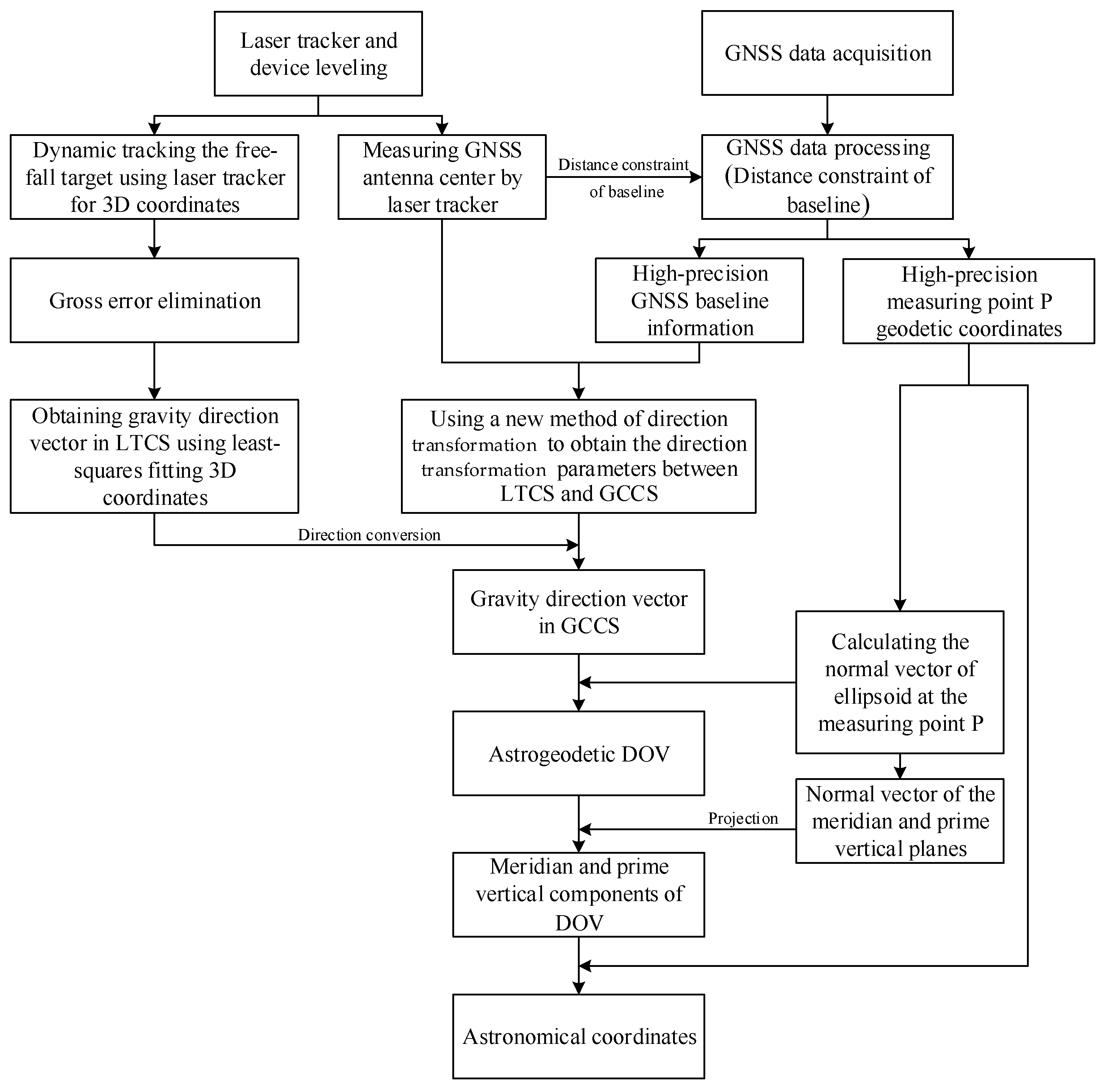
2. Principle and Methodology
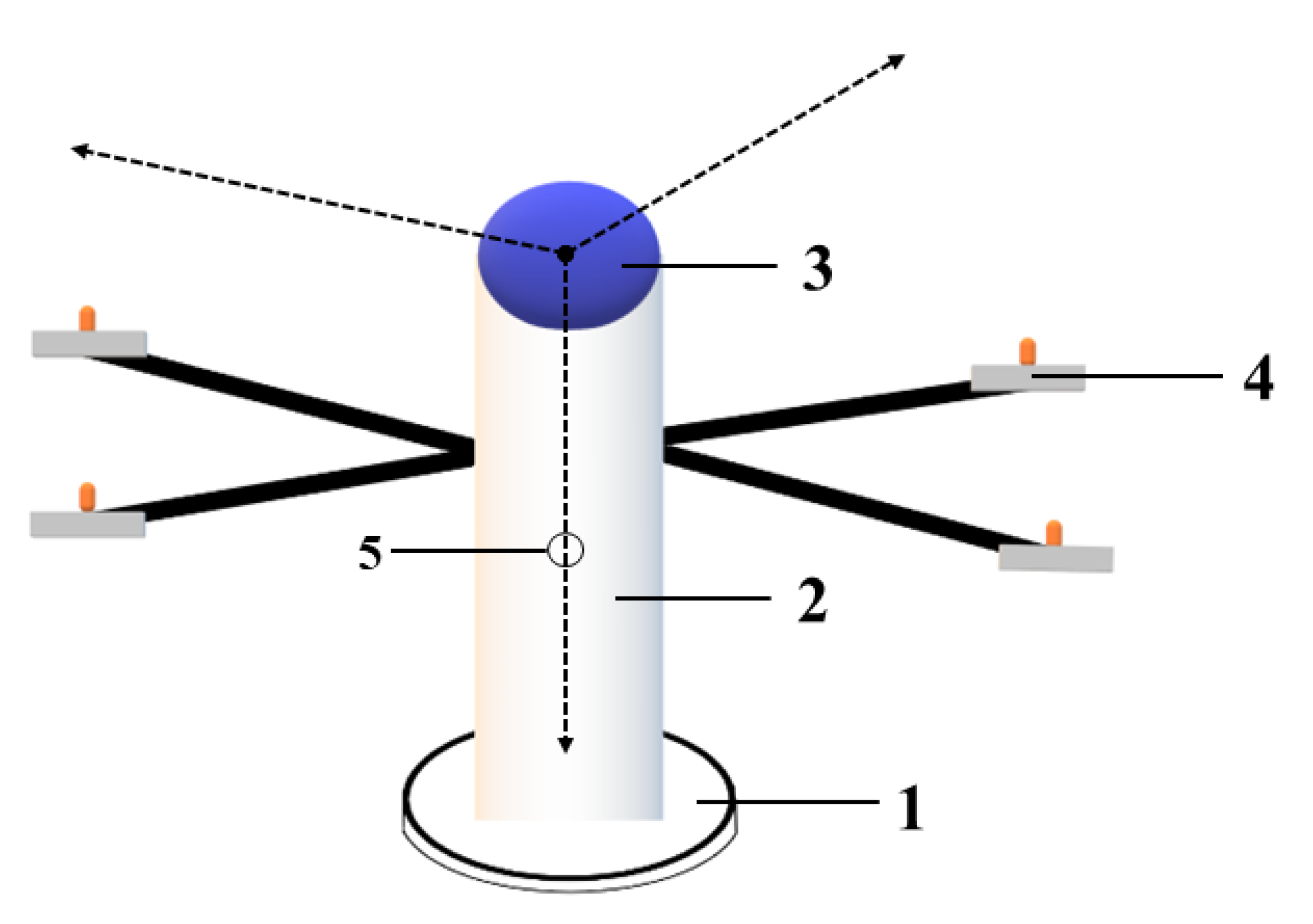
2.1. Extracting Gravity Direction Vector
2.1.1. Spatial Linear Fitting Using LS
2.1.2. Spatial Linear Fitting Using TLS
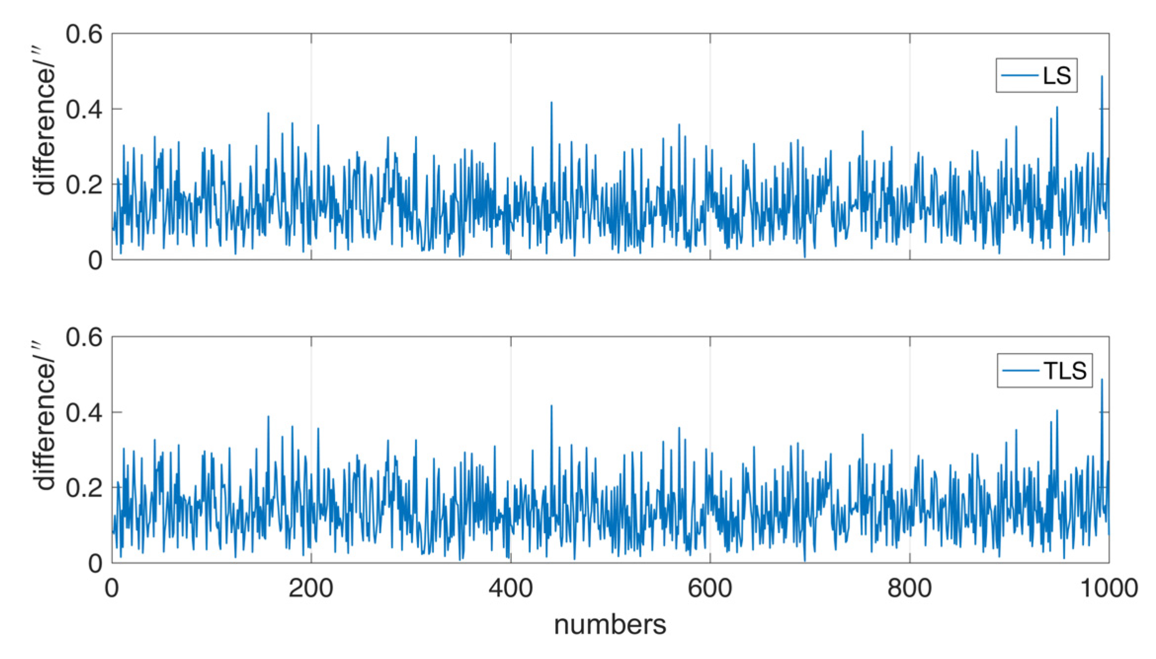
2.1.3. Comparative Analysis of LS and TLS
2.2. Space Direction Vector Transformation
- (i)
- The approximate value is generally desirable:
- (ii)
- The error equation is composed according to Equation (11), and if there are baselines, error equations can be composed.
- (iii)
- The corrections of unknowns are solved by equations.
- (iv)
- The latest values of unknowns are calculated.
- (v)
- According to the corrections, judge whether the convergence requirement is satisfied.If not, repeat steps (ii) to (v) until the convergence is satisfied.
- (vi)
- According to the rotation matrix obtained iteratively, the gravity direction vector in LTCS is converted to GCCS:where is the gravity direction vector in GCCS.
2.3. Calculation of Astrogeodetic DOV
3. Simulation Study
3.1. Theoretical Precision of DOV
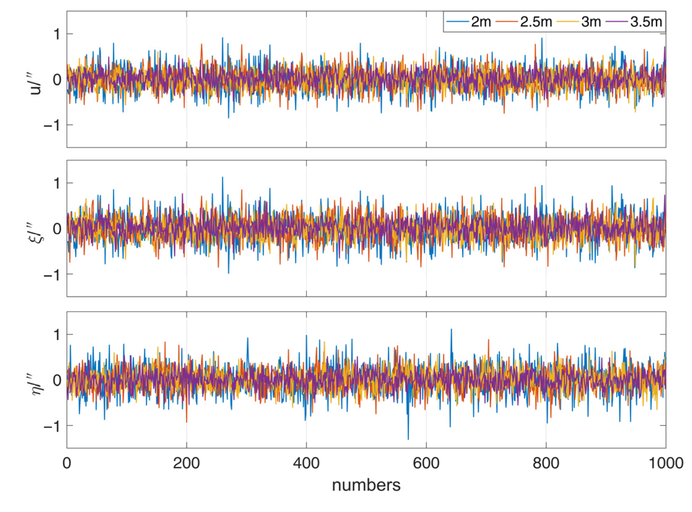
3.2. Influence of Laser Tracking Measurement Error on DOV
3.3. Influence of GNSS Error on DOV
4. Conclusions
Author Contributions
Funding
Data Availability Statement
Acknowledgments
Conflicts of Interest
References
- Tse, C.M.; Bâki Iz, H. Deflection of the vertical components from GPS and precise leveling measurements in Hong Kong. J. Surv. Eng. 2006, 132, 97–100. [Google Scholar] [CrossRef]
- Hirt, C.; Bürki, B.; Somieski, A.; Seeber, G. Modern determination of vertical deflections using digital zenith cameras. J. Surv. Eng. 2010, 136, 1–12. [Google Scholar] [CrossRef]
- Ning, J.; Guo, C.; Wang, B.; Wang, H. Refined determination of vertical deflection in China mainland area. Geomat. Inf. Sci. Wuhan Univ. 2006, 31, 1035–1038. [Google Scholar] [CrossRef]
- Li, J. The recent Chinese terrestrial digital height datum model: Gravimetric quasi-geoid CNGG2011. Acta. Geod. Cartogr. Sin. 2012, 41, 651–660. [Google Scholar] [CrossRef]
- Yuan, J.; Guo, J.; Shen, Y.; Dai, J.; Liu, X.; Kong, Q. Automatic observation of astronomical coordinates using the Shandong university of science and technology/national astronomical observatories digital zenith tube. J. Test. Eval. 2022, 50. [Google Scholar] [CrossRef]
- Ji, H.; Guo, J.; Zhu, C.; Yuan, J.; Liu, X.; Li, G. On deflections of vertical determined from HY-2A/GM altimetry data in the Bay of Bengal. IEEE J. Sel. Top. Appl. Earth Obs. Remote Sens. 2021, 14, 12048–12060. [Google Scholar] [CrossRef]
- Kühtreiber, N. Combining gravity anomalies and deflections of the vertical for a precise Austrian geoid. Boll. Geofis. Teor. Appl. 1999, 40, 545–553. [Google Scholar]
- Hirt, C.; Flury, J. Astronomical-topographic levelling using high-precision astrogeodetic vertical deflections and digital terrain model data. J. Geod. 2008, 82, 231–248. [Google Scholar] [CrossRef]
- Bányai, L. Three-dimensional adjustment of integrated geodetic observables in earth-centred and earth-fixed coordinate system. Acta Geod. Geophys. 2013, 48, 163–177. [Google Scholar] [CrossRef]
- Featherstone, W.E.; McCubbine, J.C.; Claessens, S.J.; Belton, D.; Brown, N.J. Using Ausgeoid2020 and its error grids in surveying computations. J. Spat. Sci. 2019, 64, 363–380. [Google Scholar] [CrossRef]
- Mirghasempour, M.; Jafari, A.Y. The role of astro-geodetic in precise guidance of long tunnels. Int. Arch. Photogramm. Remote Sens. Spat. Inf. Sci. 2015, 40, 453. [Google Scholar] [CrossRef] [Green Version]
- Han, Y.; Ma, L.; Hu, H.; Wang, R.; Su, Y. Application of astronomic time-latitude residuals in earthquake prediction. Earth Moon Planet 2007, 100, 125–135. [Google Scholar] [CrossRef]
- Han, S.; Sauber, J.; Luthcke, S. Regional gravity decrease after the 2010 Maule (Chile) earthquake indicates large-scale mass redistribution: Gravity change of the Maule earthquake. Geophys. Res. Lett. 2010, 37, L23307. [Google Scholar] [CrossRef]
- Soler, T.; Han, J.-Y.; Weston, N.D. On Deflection of the vertical components and their transformations. J. Surv. Eng. 2014, 140, 04014005. [Google Scholar] [CrossRef]
- Vittuari, L.; Tini, M.; Sarti, P.; Serantoni, E.; Borghi, A.; Negusini, M.; Guillaume, S. A comparative study of the applied methods for estimating deflection of the vertical in terrestrial geodetic measurements. Sensors 2016, 16, 565. [Google Scholar] [CrossRef]
- Hirt, C.; Wildermann, E. Reactivation of the venezuelan vertical deflection data set from classical astrogeodetic observations. J. S. Am. Earth Sci. 2018, 85, 97–107. [Google Scholar] [CrossRef]
- Albayrak, M.; Halıcıoğlu, K.; Özlüdemir, M.T.; Başoğlu, B.; Deniz, R.; Tyler, A.R.; Aref, M.M. The use of the automated digital zenith camera system in Istanbul for the determination of astrogeodetic vertical deflection. Bol. Ciênc. Geod. 2019, 25, e2019025. [Google Scholar] [CrossRef]
- Hirt, C.; Seeber, G. Accuracy analysis of vertical deflection data observed with the Hannover digital zenith camera system TZK2-D. J. Geod. 2008, 82, 347–356. [Google Scholar] [CrossRef]
- Guo, J.; Song, L.; Chang, X.; Liu, X. Vertical deflection measure with digital zenith camera and accuracy analysis. Geomat. Inf. Sci. Wuhan Univ. 2011, 36, 1085–1088. [Google Scholar] [CrossRef]
- Gayvoronsky, S.V.; Kuzmina, N.V.; Tsodokova, V.V. High-accuracy determination of the earth’s gravitational field parameters using automated zenith telescope. In Proceedings of the 2017 24th Saint Petersburg International Conference on Integrated Navigation Systems (ICINS), St. Petersburg, Russia, 29–31 May 2017; pp. 1–4. [Google Scholar]
- Tian, L.; Guo, J.; Han, Y.; Lu, X.; Liu, W.; Wang, Z.; Wang, B.; Yin, Z.; Wang, H. Digital zenith telescope prototype of China. Chin. Sci. Bull. 2014, 59, 1978–1983. [Google Scholar] [CrossRef]
- Hauk, M.; Hirt, C.; Ackermann, C. Experiences with the Qdaedalus System for astrogeodetic determination of deflections of the vertical. Surv. Rev. 2016, 49, 294–301. [Google Scholar] [CrossRef]
- Schwarz, K.P.; Sideris, M.G.; Forsberg, R. The use of FFT techniques in physical geodesy. Geophys. J. Int. 1990, 100, 485–514. [Google Scholar] [CrossRef]
- Liu, Q.W.; Li, Y.C.; Sideris, M.G. Evaluation of deflections of the vertical on the sphere and the plane: A comparison of FFT techniques. J. Geod. 1997, 71, 461–468. [Google Scholar] [CrossRef]
- Hirt, C.; Schmitz, M.; Feldmann-Westendorff, U.; Wübbena, G.; Jahn, C.-H.; Seeber, G. Mutual validation of GNSS height measurements and high-precision geometric-astronomical leveling. GPS Solut. 2011, 15, 149–159. [Google Scholar] [CrossRef]
- Sawyer, D.S.; Fronczek, C. Laser tracker compensation using displacement interferometry. Am. Soc. Precis. Eng. 2003, 30, 351–358. [Google Scholar]
- Hexagon Metrology. Leica Laser Tracker Systems. 2022. Available online: https://www.hexagonmi.com/products/laser-tracker-systems (accessed on 6 June 2022).
- Strutz, T. Data Fitting and Uncertainty (a Practical Introduction to Weighted Least Squares and Beyond); Springer: Berlin/Heidelberg, Germany, 2010. [Google Scholar]
- Bühlmann, P.L.; Geer, S. Statistics for High-Dimensional Data: Methods, Theory and Applications; Teubner Verlag: Wiesbaden, Germany, 2011. [Google Scholar]
- Malissiovas, G.; Neitzel, F.; Petrovic, S. Götterdämmerung over total least squares. J. Geod. Sci. 2016, 6, 43–60. [Google Scholar] [CrossRef]
- Chen, Y.; Shen, Y.; Liu, D. A simplified model of three dimensional datum transformation adapted to big rotation angle. Geomat. Inf. Sci. Wuhan Univ. 2004, 29, 1101–1105. [Google Scholar]
- Wang, Q.; Chang, G.; Xu, T.; Zou, Y. Representation of the rotation parameter estimation errors in the Helmert transformation model. Surv. Rev. 2018, 50, 69–81. [Google Scholar] [CrossRef]


| MAX | MIN | MEAN | STD | RMS | |
|---|---|---|---|---|---|
| LS | 0.192 | 0.102 | 0.146 | 0.014 | 0.146 |
| TLS | 0.192 | 0.102 | 0.146 | 0.014 | 0.146 |
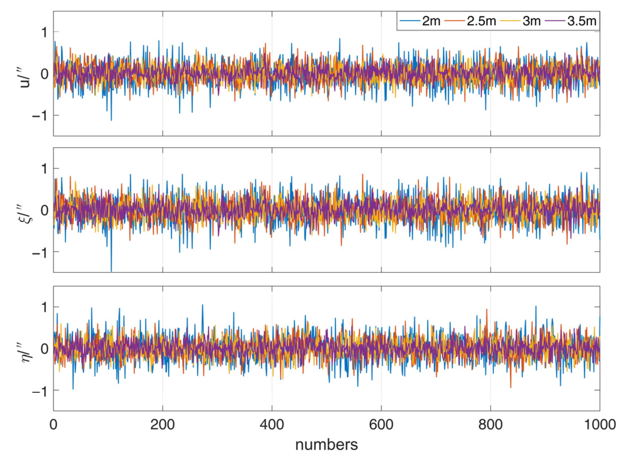
| Radius r | 2 m | 2.5 m | 3 m | 3.5 m | |
|---|---|---|---|---|---|
| u | MAX | 0.91 | 0.78 | 0.63 | 0.72 |
| MIN | −0.85 | −0.75 | −0.72 | −0.48 | |
| MEAN | 0.00 | −0.01 | −0.01 | 0.01 | |
| STD | 0.28 | 0.24 | 0.20 | 0.17 | |
| RMS | 0.28 | 0.24 | 0.20 | 0.17 | |
| ξ | MAX | 1.13 | 0.91 | 0.69 | 0.76 |
| MIN | −0.99 | −0.85 | −0.84 | −0.65 | |
| MEAN | −0.01 | −0.01 | −0.01 | 0.02 | |
| STD | 0.32 | 0.28 | 0.23 | 0.20 | |
| RMS | 0.32 | 0.28 | 0.23 | 0.20 | |
| η | MAX | 1.12 | 0.88 | 0.83 | 0.54 |
| MIN | −1.31 | −0.93 | −0.65 | −0.55 | |
| MEAN | 0.00 | 0.00 | 0.00 | 0.00 | |
| STD | 0.33 | 0.25 | 0.22 | 0.19 | |
| RMS | 0.33 | 0.25 | 0.22 | 0.19 |
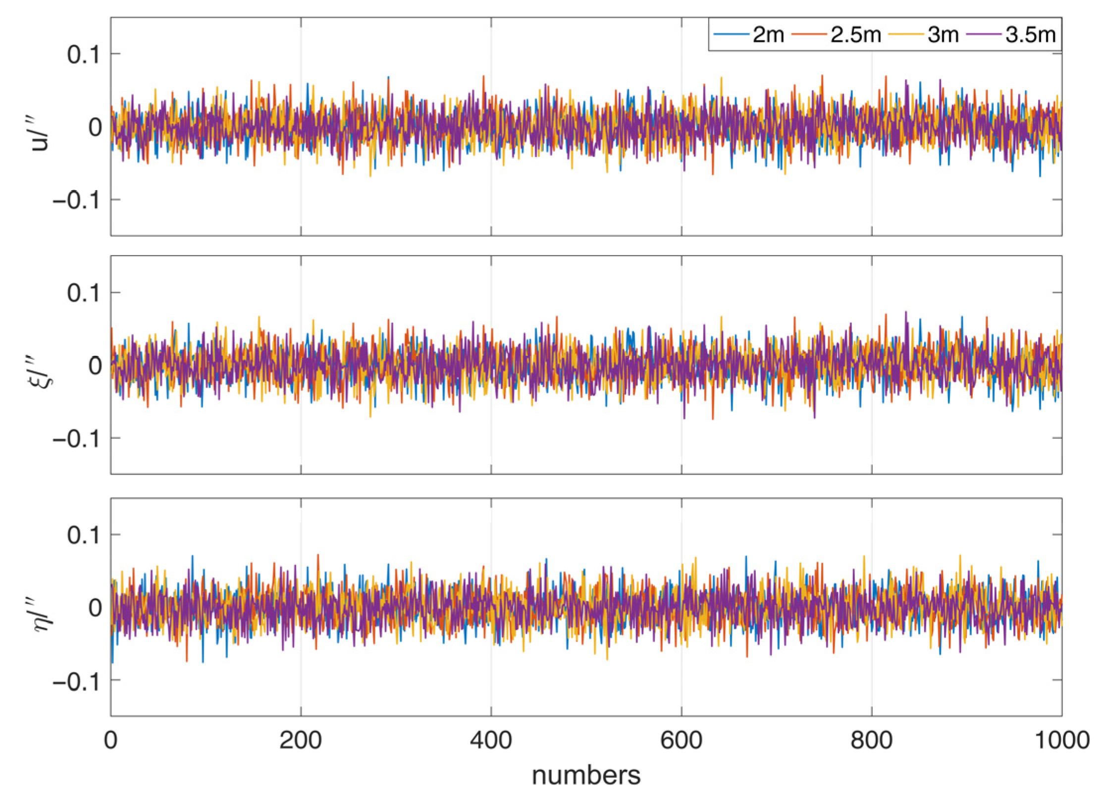
| Radius r | 2 m | 2.5 m | 3 m | 3.5 m | |
|---|---|---|---|---|---|
| u | MAX | 0.07 | 0.07 | 0.07 | 0.06 |
| MIN | −0.07 | −0.07 | −0.07 | −0.06 | |
| MEAN | 0.00 | 0.00 | 0.00 | 0.00 | |
| STD | 0.02 | 0.02 | 0.02 | 0.02 | |
| RMS | 0.02 | 0.02 | 0.02 | 0.02 | |
| ξ | MAX | 0.07 | 0.07 | 0.07 | 0.07 |
| MIN | −0.06 | −0.07 | −0.07 | −0.07 | |
| MEAN | 0.00 | 0.00 | 0.00 | 0.00 | |
| STD | 0.02 | 0.02 | 0.02 | 0.02 | |
| RMS | 0.02 | 0.02 | 0.02 | 0.02 | |
| η | MAX | 0.07 | 0.07 | 0.07 | 0.06 |
| MIN | −0.08 | −0.07 | −0.07 | −0.07 | |
| MEAN | 0.00 | 0.00 | 0.00 | 0.00 | |
| STD | 0.02 | 0.02 | 0.02 | 0.02 | |
| RMS | 0.02 | 0.02 | 0.02 | 0.02 |
| Radius r | 2 m | 2.5 m | 3 m | 3.5 m | |
|---|---|---|---|---|---|
| u | MAX | 0.81 | 0.73 | 0.58 | 0.50 |
| MIN | −0.83 | −0.69 | −0.57 | −0.57 | |
| MEAN | 0.01 | 0.00 | 0.00 | 0.00 | |
| STD | 0.29 | 0.25 | 0.20 | 0.17 | |
| RMS | 0.29 | 0.25 | 0.20 | 0.17 | |
| ξ | MAX | 1.00 | 0.86 | 0.68 | 0.59 |
| MIN | −1.04 | −0.86 | −0.63 | −0.68 | |
| MEAN | 0.00 | 0.00 | 0.00 | 0.00 | |
| STD | 0.33 | 0.28 | 0.23 | 0.20 | |
| RMS | 0.33 | 0.28 | 0.23 | 0.20 | |
| η | MAX | 1.05 | 0.94 | 0.61 | 0.53 |
| MIN | −0.98 | −0.94 | −0.74 | −0.48 | |
| MEAN | 0.01 | 0.00 | 0.00 | 0.01 | |
| STD | 0.32 | 0.25 | 0.21 | 0.18 | |
| RMS | 0.32 | 0.25 | 0.21 | 0.18 |
Publisher’s Note: MDPI stays neutral with regard to jurisdictional claims in published maps and institutional affiliations. |
© 2022 by the authors. Licensee MDPI, Basel, Switzerland. This article is an open access article distributed under the terms and conditions of the Creative Commons Attribution (CC BY) license (https://creativecommons.org/licenses/by/4.0/).
Share and Cite
Jin, X.; Liu, X.; Guo, J.; Zhou, M.; Wu, K. A Novel All-Weather Method to Determine Deflection of the Vertical by Combining 3D Laser Tracking Free-Fall and Multi-GNSS Baselines. Remote Sens. 2022, 14, 4156. https://doi.org/10.3390/rs14174156
Jin X, Liu X, Guo J, Zhou M, Wu K. A Novel All-Weather Method to Determine Deflection of the Vertical by Combining 3D Laser Tracking Free-Fall and Multi-GNSS Baselines. Remote Sensing. 2022; 14(17):4156. https://doi.org/10.3390/rs14174156
Chicago/Turabian StyleJin, Xin, Xin Liu, Jinyun Guo, Maosheng Zhou, and Kezhi Wu. 2022. "A Novel All-Weather Method to Determine Deflection of the Vertical by Combining 3D Laser Tracking Free-Fall and Multi-GNSS Baselines" Remote Sensing 14, no. 17: 4156. https://doi.org/10.3390/rs14174156
APA StyleJin, X., Liu, X., Guo, J., Zhou, M., & Wu, K. (2022). A Novel All-Weather Method to Determine Deflection of the Vertical by Combining 3D Laser Tracking Free-Fall and Multi-GNSS Baselines. Remote Sensing, 14(17), 4156. https://doi.org/10.3390/rs14174156