Study on the Impact of Spatial Resolution on Fractional Vegetation Cover Extraction with Single-Scene and Time-Series Remote Sensing Data

Abstract

The spatial resolution of remote sensing images directly affects the accuracy, efficiency, and computational cost of extracting the fractional vegetation cover (FVC). Taking the Liyang woodland region, Jiangsu Province, as the study area, FVCs with varying spatial resolutions were extracted separately from Sentinel-2, Landsat-8, MOD13Q1, and MOD13A1. The variations in FVCs extracted from remote sensing images with varying spatial resolutions were analyzed at one specific time and time series within a year. The results show that (i) the overall mean FVC values of the four spatial resolution images did not differ substantially; however, FVCs with varying spatial resolutions present with a regular pattern of overestimation or underestimation at different vegetation levels. (ii) Taking the 10 m spatial resolution FVC as the reference, the accuracy values of FVC extraction at 30 m, 250 m, and 500 m resolutions were 91.0%, 76.3%, and 76.7%, respectively. The differences in the spatial distribution of FVCs are the most obvious at water–land interfaces and at the edge of each woodland patch. (iii) The highest accuracy of time-series FVC extraction from lower-resolution images is in the range of 0.6~0.7 for FVC. The degree of variation in FVC of time series varying spatial resolutions depends on the season and vegetation cover conditions. In summary, there are considerable differences in the need to monitor high-resolution images depending on the FVC level of the land surface. This study provides a reference for selection and accuracy research of remote sensing images for FVC extraction.

1. Introduction

The ratio of the vertical projected vegetated area to the total ground area, termed fractional vegetation cover (FVC), is a commonly used indicator for terrestrial ecosystems and vegetation degradation [1,2,3,4]. FVC has been widely used in monitoring soil erosion, desertification, and climate change [5,6,7,8]. In recent years, with the rapid development of remote sensors, remote sensing images have become the main data source for FVC acquisition due to their advantages of wide coverage, low acquisition cost, and multitemporal nature [9].

The variety of resolutions of remote sensing images provides many options for FVC extraction, in addition to difficulty in choosing an appropriate data source. Generally, FVCs extracted from fine-spatial-resolution images (i.e., less than 10 m) are essential for regional-scale vegetation research, whereas FVCs with coarse--resolution images (i.e., resolutions of hundreds to thousands of meters) are predominantly used in research on global vegetation change [10]. Remote sensing data with coarse spatial resolutions, such as SPOT VEGETATION (1000 m) and MODIS (250 m and 500 m) usually have a high frequency of revisits, enabling detection of vegetation changes (e.g., during the growing season) at a higher frequency. However, due to coarse spatial resolutions, it is difficult to capture the precise spatial distributions of vegetation in highly heterogeneous and complex terrain, which affects the accuracy of vegetation information extraction [11] and inhibits the detection of feature differences at small scales [12,13]. However, the use of data with fine spatial resolutions to monitor vegetation change is often limited due to problems such as long revisit periods, vulnerability to weather effects, and high computational cost. At present, the monitoring of vegetation in a cost-effective manner, at a fine spatial scale, and over relatively large areas remains a significant challenge [14]. Therefore, it is necessary to investigate the differences between FVCs extracted from remote sensing images with various spatiotemporal resolutions, so as to select proper data sources and improve the efficiency of FVC extraction for specific applications.

Many studies have been conducted on the impact of spatial resolution on FVC extraction. Zhang et al. [15] studied the influence of image resolutions on FVCs extracted from five remote sensing datasets, including SPOT, MODIS, Landsat TM, ALOS, and IKONOS. The results showed that data with varying spatial resolutions are applicable to different regional scales. Images with a 30 m resolution were proven to be the most applicable to small-watershed scales. By comparing FVC derived from high-resolution data, Mu et al. [16] found that the use of coarse-resolution remote sensing data (i.e., 1 km resolution) resulted in the overestimation of the FVC of crops in their study area. Qi et al. [17] extracted FVC in the San Diego watershed using Landsat-8 TM and SPOT4 VEGETATION images. The results demonstrated that the mean values of the FVC were accurate at different spatial scales. However, due to the spatial heterogeneity of the land surface, the effect of spatial resolution may differ for subareas with varying FVC levels [18]. In addition, the FVC changes within an annual cycle correspond to normal vegetation growth. The FVC of a given pixel changes with vegetation growth. Therefore, the differences between FVC time-series with different spatial resolutions is worth extensively studying, especially for applications in which the long-term monitoring of FVC is crucial, such as soil erosion risk assessment, monitoring of natural hazards, and climate modeling [19,20,21].

As a whole, the aforementioned studies of FVC comparisons and validations are confined to the overall regional accuracy of multi-spatial resolution data at one specific time. Therefore, the main objective of this study is to study the variation in FVCs extracted from remote sensing images with different spatial resolutions, not only at one specific time but also considering the normal growth of vegetation within a year. The data used in this study include Sentinel-2, Landsat-8, MOD13Q1, and MOD13A1 remote sensing images. In order to study the variation in FVC level at one specific time, confusion matrices were used to compare the effect of spatial resolution on subareas with different FVC levels. Furthermore, the enhanced spatial and temporal adaptive reflectance fusion model [22] was used to produce an FVC time-series dataset, on the basis of which the differences between FVC time series with different spatial resolutions were evaluated. The results of this study are expected to provide a reference for the selection of remote sensing images for FVC extraction and the study of FVC accuracy.

2. Materials and Methods

2.1. Study Area

Liyang is a city located in the west of the Taihu Lake Basin between 31°01′–31°41′N and 119°08′–119°36′E. It covers an area of approximately 1535 km². Woodland covers 249 km², mainly distributed in the hilly areas to the north and south, with plain areas in the central and eastern regions (Figure 1). There are many geomorphic types represented in Liyang, including low mountains, hills, and polders. The southern part of Liyang consists of the Yili mountainous area and the northwestern part of the LiBei mountainous area.

In terms of climate, Liyang is located in the transition zone between the central subtropics and the northern subtropics, with an annual average temperature of 15.5 °C and an average annual rainfall of 1005~1136 mm. Owing to such a warm and humid climate, diverse plant species grow in this area [23].

The woodland in Liyang mainly contains four types of forests: broad-leaved forest, coniferous forest, mixed coniferous forest, and bamboo forest, among which broad-leaved forest and bamboo forest are the dominant types. Specifically, the broad-leaved forests include evergreen broad-leaved forests, deciduous broad-leaved forests, and mixed evergreen–deciduous broad-leaved forests. The evergreen broad-leaved forests are dominated by Lithocarpus glaber. The deciduous broad-leaved forests are dominated by Quercus acutissima and Liquidamba formosana. The evergreen–deciduous broad-leaved mixed forests are dominated by Phoebe sheareri and Quercus acutissima. Bamboo forests mainly contain Phyllostachys heterocycla and Phyllostachys viridis [24]. According to the Forest Resources Survey in Liyang, the area of timber forest is 101.6 km², comprising 71.5% bamboo forest. The broad-leaved forest, coniferous forest, and mixed coniferous forest mainly serve as public recreational forests, accounting for 41.3% of the total area of woodland.

2.2. Data Sources

The data used in this study include Sentinel-2, Landsat-8, MOD13Q1, and MOD13A1 remote sensing images, which can be downloaded for free from the European Space Agency (https://scihub.copernicus.eu/dhus/, accessed on 3 October 2021) and the USGS website (https://earthexplorer.usgs.gov/, accessed on 4 October 2021). To ensure data quality, only images with cloud cover of less than 10% were considered. Given the impact of weather conditions, images acquired in 2017 were used in this study, as this year has the best overall data quality of the past 5 years (

Table 1. Details of the remote sensing images used in this study.

Data Source	Spatial Resolution (m)	Temporal Resolution (d)	Date of Images (mm/dd)	No. of Images
Sentinel-2	10	5	07/28	1
Landsat-8	30	16	01/26, 02/11, 03/15, 05/18, 07/21, 10/09, 10/25, 11/26, 12/12	9
MOD13Q1	250	16	01/01, 01/17, 02/02, 02/18, 03/06, 03/22, 04/07, 04/23, 05/09, 05/25, 06/10, 06/26, 07/12, 07/28, 08/13, 08/29, 09/14, 09/30, 10/16, 11/01, 11/17, 12/03, 12/19	23
MOD13A1	500	16	01/01, 01/17, 02/02, 02/18, 03/06, 03/22, 04/07, 04/23, 05/09, 05/25, 06/10, 06/26, 07/12, 07/28, 08/13, 08/29, 09/14, 09/30, 10/16, 11/01, 11/17, 12/03, 12/19	23

).

Because most vegetation is at its climax in summer, the influence of soil on FVC can be minimized compared to other seasons. Therefore, the Sentinel-2 image data on 28 July have the best quality in summer. The Sentinel-2 image from this date was used as a reference image to compare the variation in FVCs extracted from remote sensing images with different spatial resolutions on the aforementioned date. A total of 9 Landsat-8 images that meet the quality standard were used, and the image from 21 July was used for FVC-level analysis. MOD13Q1 and MOD13A1 image data from the image taken on 28 July were used for FVC-level analysis. The full-year data of Landsat-8 (the remaining 14 images were obtained by ESTARFM model), MOD13Q1, and MOD13A1 were used for time-series analysis.

2.3. FVC Extraction and Classification

The pixel dimidiate model is a commonly used for FVC estimation [25]. In this model, pixel information is composed of green vegetation information and soil contribution information. FVC can be defined as the weight of vegetation in a pixel. Currently, the Normalized Difference Vegetation Index (NDVI) is a common indicator of vegetation growth, which correlates well with vegetation coverage [26]. NDVI was calculated using near-infrared (NIR) and red reflectance data, i.e.,

$$\mathrm{NDVI}=\frac{{\rho }_{nir}-{\rho }_r}{{\rho }_{nir}+{\rho }_r}$$

(1)

$$\mathrm{FVC}=\frac{NDVI-NDV{I}_{Soil}}{NDV{I}_{Veg}-NDV{I}_{Soil}}$$

(2)

where ${\rho }_r$ and ${\rho }_{nir}$ represent surface reflectances averaged over visible and NIR regions of the spectrum, respectively; $NDV{I}_{Soil}$ is the NDVI value of a pure soil pixel; and $NDV{I}_{Veg}$ is the NDVI value of a pure vegetation pixel. In this study, the upper and lower thresholds of NDVI were calculated with 95% confidence intervals to approximate the values of $NDV{I}_{Soil}$ and $NDV{I}_{Veg}$, respectively [27,28].

According to the “standards for classification and gradation of soil erosion” promulgated by the Ministry of Water Resources in 2007 [29], we divided the woodland FVC into 5 levels.

Table 2. Classification of fractional vegetation cover (FVC) level in the study area.

Coverage Level	Name	FVC (%)
I	Low coverage	<30
II	Medium-low coverage	30–45
III	Medium coverage	45–60
IV	Medium-high coverage	60–75
V	High coverage	≥75

lists the details of the FVC levels.

2.4. Analysis of FVC

In reference to the principle of confusion matrix [30,31,32], the differences in FVC levels between Sentinel-2 and Landsat-8, MOD13Q1, and MOD13A1 images were assessed quantitatively. The confusion matrix contains information about the reference image and analyzed image classifications according to a classification system (Table 2). Formula (3) presents the basic form of the confusion matrix for the FVC multilevel classification task, with the levels $L_1$, $L_2,$ and $L_n$ (n = 5). In this confusion matrix, $S_{ij}$ represents the area of FVC belonging to level $L_i$ in the reference image but classified as level $L_j$ in the analyzed image.

$$\begin{array}{c}\begin{array}{cccccc}& L_1& \cdots & L_j& \cdots & L_n\end{array}\\ \begin{array}{c}{L}_1\\ ⋮\\ L_i\\ ⋮\\ L_j\end{array}\left[\begin{array}{ccccc}{S}_{11}& \cdots & S_{1j}& \cdots & S_{1n}\\ ⋮& & ⋮& \ddots & ⋮\\ S_{i1}& \cdots & S_{ij}& \cdots & S_{in}\\ ⋮& & ⋮& & ⋮\\ S_{n1}& \cdots & S_{nj}& \cdots & S_{nn}\end{array}\right]\end{array}$$

(3)

Accordingly, overall accuracy (Formula (4)) refers to the total accuracy of FVC extraction from the analyzed image based on FVC_10m. User’s accuracy (Formula (5)) refers to the percentage of FVC level correctly determined in the reference image. Producer’s accuracy (Formula (6)) refers to percentage of the FVC level in the reference image that is correctly classified. OA represents overall accuracy. UA represents user’s accuracy. PA represents producer’s accuracy.

$$\mathrm{OA}=\frac{S_{11}+\dots +S_{ij}+\dots +S_{nn}}{S}$$

(4)

$$\mathrm{UA}=\frac{S_{ij}}{S_{in}}$$

(5)

$$\mathrm{PA}=\frac{S_{ij}}{S_{nj}}$$

(6)

2.5. Generation of Time-Series FVC

Due to unfavorable weather conditions, 14 high-quality Landsat-8 time-series images were missed in 2017. In the present study, the Enhanced Spatial and Temporal Adaptive Reflectance Fusion Model (ESTARFM) proposed by Zhu [22] was used to generate 30 m spatial resolution image time series. ESTARFM was modified from the STARFM algorithm presented by Gao [33] by introducing the conversion coefficient and adjusting the equations of weight to improve the fusion accuracy of the algorithm in heterogeneous areas [22]. The ESTARFM can predict target pixels, fully taking into account the adjacent pixels and the target pixel according to three factors: the geographical distance, the spectral difference, and the temporal difference. The ESTARFM model inputs high-spatial-resolution and high-temporal-resolution data from two consecutive periods, inputs high-temporal-resolution data from a target period, and uses these to generate high-spatial-resolution data for the target period.

Several studies have shown that the accuracy of fusion models assessed using a vegetation index is generally higher when performing a direct fusion of the index than when performing fusion of the reflectance first and then deriving the index [34,35,36]; therefore, in the present study, vegetation indices from the two datasets (MOD13AI and Landsat-8 NDVI) were fused directly. First, to determine the size of the window, two Landsat-8 NDVI images were used to select the pixels similar to the target pixels in the search window. The weights of the similar pixels were calculated to determine the contributions of similar pixels to the target pixel. Then, a linear regression was used to calculate the conversion coefficients of similar pixels. Finally, both the weights and conversion coefficients of similar pixels were used to calculate the high spatiotemporal resolution of the predicted NDVI based on the MOD13AI at the prediction time.

In essence, the ESTARFM model moves an entire image, one pixel at a time, through a window with a size of w, thereby determining the prediction value of the pixel at the center of the movement one by one. The prediction value of the center pixel is expressed as (Equation (7)):

$$\begin{array}{cc}\hfill L\left(x_{w/2},y_{w/2},t_p,B\right)& \\ & =L\left(x_{w/2},y_{w/2},t_0,B\right)+{\displaystyle {\displaystyle \sum }_{i=1}^N}{W}_i\times V_i\times (M\left(x_I,I,t_p,B\right)\hfill \\ & -M\left(I_i,I,t_0,B\right))\hfill \end{array}$$

(7)

where $L\left(x_{w/2},y_{w/2},t_p,B\right)$ and $L\left(x_{w/2},y_{w/2},t_0,B\right)$ denote the fine-resolution reflectance of the central pixel of band B in prediction data ($t_p$) and observed data ($t_0$), respectively; $M\left(x_i,y_i,t_p,B\right)$ and $M\left(x_I,y_i,t_0,B\right)$ denote the coarse-resolution reflectance of the pixels located at ($x_i,y_i$) of band B of the prediction data ($t_p$) and observed data ($t_0$), respectively; w is the size of the search window; ($x_{w/2}$, $y_{w/2}$) is the fine-resolution reflectance of the central pixel; N is the number of similar pixels, including the central prediction pixel; ($x_i,y_i$) is the location of ith similar pixel; $W_i$ is the weight of ith similar pixel; and $V_i$ is the conversion coefficient of ith similar pixel.

3. Results

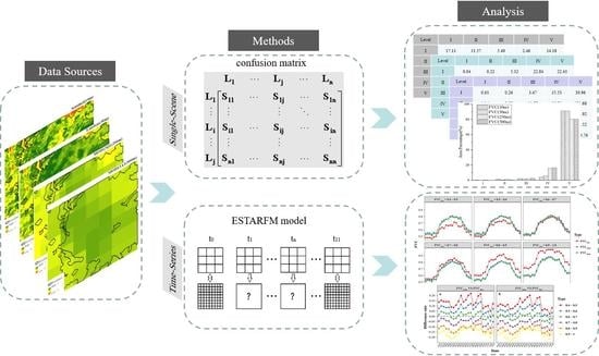
3.1. FVC Extraction Using Different Spatial Resolutions

Four images with similar acquisition dates (Sentinel-2, MOD13Q1, and MOD13A1 images obtained on 28 July 2017 and the Landsat-8 image obtained on 21 July 2017) were used to extract the FVC of the study area. Figure 2 compares the results within a sample site mainly consisting of woodland (a total of 2100 pixels). For FVCs extracted from the Sentinel-2 and Landsat-8 images, the overall spatial distribution of vegetation is basically consistent. The FVC spatial distribution is clearer with images of higher spatial resolution. When the image resolution is reduced to 250 m and 500 m, the woodland boundaries are blurred, and the spatial distribution information of the FVCs is significantly lost.

According to the statistical results from the sample site (

Table 3. Statistics of FVCs extracted from images of different spatial resolution from the sample site shown in Figure 2.

Statistic	FVC10m	FVC30m	FVC250m	FVC500m
Maximum	1	1	0.85	0.82
Minimum	0	0	0.41	0.60
Mean ± SE	0.76 ± 0.0044	0.74 ± 0.0033	0.74 ± 0.0019	0.73 ± 0.0015
Standard deviation	0.20	0.15	0.09	0.07

), the maximum and minimum values of FVC extracted from 10 m and 30 m resolution images are equal. However, as the image resolution decreases, the range of FVC values indicates a decrease in the maximum values and an increase in the minimum values. The FVC mean values for the four resolutions do not vary substantially, but the standard deviations decrease gradually as the resolution is reduced. The maps of woodland FVC in Liyang at different resolutions (Figure 3) show that the spatial distributions of FVC_30m and FVC_10m are similar, whereas the spatial distributions of FVC_250m and FVC_500m are similar but with obvious differences relative to FVC_10m. Differences between the FVC distributions are most evident along the edges of woodland patches, as well as around the woodlands near Shahe Reservoir and Daxi Reservoir in Tianmuhu township (see Figure 1b for location).

To better understand the spatial distribution of differences among the FVCs extracted using different spatial resolutions, deviation of FVC at 30 m, 250 m, and 500 m spatial resolutions from FVC at 10 m spatial resolution were calculated (Figure 4). We found that the difference between FVC_30m and FVC_10m mainly occurs at lower values, ranging from −0.1 to 0.1. The differences between FVC_250m and FVC_10m and between FVC_500m and FVC_10m mainly occur at higher values, ranging from −0.4 to −0.1. The differences between Sentinel-2 and MOD13Q1/MOD13A FVCs are most obvious in Tianmuhu, especially at the edges of woodland patches. In these areas, the difference can reach −0.4 to −0.1, indicating an underestimation of the FVCs extracted from MOD13Q1 and MOD13A1 images relative to the FVCs extracted from 10 m Sentinel-2 images.

3.2. Comparison of FVC-Level Distribution

FVCs were classified into five levels according to classification standards (Table 2). The proportion of each FVC level was calculated as shown in Figure 5. The percentage of each FVC level varies depending on the spatial resolution. Specifically, the percentages of FVC_30m and FVC_10m are similar across all levels. The area of level V at both spatial resolutions accounts for more than 90%. The difference in the area percentage of level II and level IV is quite small for the two spatial resolutions. These results indicate that the ability of the Landsat-8 image to reflect the FVC level in the region is similar to that of the Sentinel-2 image. The percentages of FVC_250m and FVC_500m are quite similar but differ considerably from those of FVC_10m. The percentage of level IV is significantly higher than that of FVC_10m, representing an approximate difference of 11%. The percentage of level V is remarkably lower than that of FVC_10m, with a difference of approximately 12%. However, levels I, II, and III do not differ considerably.

Taking FVC_10m as a reference,

Table 4. Areas (ha) of misclassification of the five coverage levels derived from FVC_30m values.

Level	I	II	III	IV	V
I	17.13	11.57	5.49	2.46	14.18
II	11.68	54.79	48.26	15.44	64.08
III	0.85	24.98	98.48	94.87	78.92
IV	0.25	5.56	63.66	230.19	267.64
V	0.04	1.35	41.23	416.81	11,403.65

,

Table 5. Areas (ha) of misclassification of the five coverage levels derived from FVC_250m values.

Level	I	II	III	IV	V
I	0.61	0.26	3.47	15.53	30.96
II	1.14	2.92	11.77	56.74	121.68
III	1.17	4.62	17.66	89.73	184.92
IV	2.27	7.27	29.59	151.65	376.52
V	37.06	121.29	227.81	1753.16	9723.76

and

Table 6. Areas (ha) of misclassification of the five coverage levels derived from FVC_500m values.

Level	I	II	III	IV	V
I	0.04	0.22	5.32	22.84	22.41
II	0.31	3.69	11.19	68.66	110.40
III	0.41	5.92	14.22	99.99	177.56
IV	0.58	8.08	26.14	165.20	367.30
V	7.54	44.58	256.06	1785.59	9769.31

represent the misclassified area for five levels of FVC_30m, FVC_250m, and FVC_500m, respectively (see Equation (3) for more detail).

Table 7. Accuracy of woodland FVC (I to V) results. Sentinel-2 images with a resolution of 10 m were used as the reference. See Table 2 for a definition of the coverage levels.

Accuracy	30 m		250 m		500 m
	PA(%)	UA(%)	PA(%)	UA(%)	PA(%)	UA(%)
I	33.7	57.2	1.2	1.4	0.1	0.5
II	28.2	55.8	1.5	2.1	1.9	5.9
III	33.0	38.3	5.9	6.1	4.8	4.5
IV	40.6	30.3	26.7	7.3	29.1	7.7
V	96.1	96.4	82.0	93.2	82.4	93.5

presents the PA and UA for three spatial resolutions (see Equations (5) and (6)). The overall accuracy values of FVC_30m, FVC_250m, and FVC_500m were calculated according to Equation (4), totaling 91.0%, 76.3%, and 76.7%, respectively.

The overall accuracy of FVC_30m is the highest, whereas the overall accuracy of FVC_250m and FVC_500m is not much lower. Regarding the misclassification of each FVC level (Table 4, Table 5 and Table 6), the difference in FVC_30m is mainly caused by misclassification into adjacent higher coverage levels. In comparison, the differences in FVC_250m and FVC_500m are mainly caused by misclassification into higher coverage levels, showing that compared to FVC_10m, the FVCs extracted from all three resolution images are overestimated. However, the overestimation is greater in FVC_250m and FVC_500m than in FVC_30m.

As shown by the extraction accuracy of each coverage level (Table 7), with increased FVC, the overall PA and UA of FVC_30m, FVC_250m, and FVC_500m improve. In addition, the extraction accuracy of level V is much higher than that of the other levels. The PA and UA at each level of FVC_30m are higher than those of FVC_250m and FVC_500m. Among these, the difference in extraction accuracy of level II is greatest, with a smaller difference in extraction accuracy of level V. This indicates that the magnitude of FVC can have a considerable impact on the accuracy of FVC extraction.

3.3. Comparison of FVC Time Series

Considering that the quality of the Sentinel-2 images is sensitive to weather and the immaturity of the spatiotemporal fusion method for acquiring 10 m resolution time-series images, in this study, time-series images with 30 m spatial resolution were generated using ESTARFM, as FVC_30m is most similar to the FVC_10m reference data. The time series of FVC_30m, FVC_250m, and FVC_500m were compared in order to study the impact of image resolution on FVC time series.

After screening, nine periods of high-quality (cloud cover less than 10%) raw Landsat-8 data remained (

Table 8. List of dates of images used in the ESTARFM model to generate NDVI time series.

No.	Date of Predicted Data (500 m Resolution)	Date of Input Data		Date of Output Data (30 m Resolution)
		MOD13A1	Landsat NDVI
1	01/01	02/02, 02/18	01/26, 02/11	01/01
2	01/17	02/02, 02/18	01/26, 02/11	01/17
3	-	-	-	-
4	-	-	-	-
5	03/06	03/22, 05/25	03/15, 05/18	03/06
6	-	-	-	-
7	04/07	03/22, 05/25	03/15, 05/18	04/07
8	04/23	03/22, 05/25	03/15, 05/18	04/23
9	05/09	05/25, 07/28	05/18, 07/21	05/09
10	-	-	-	-
11	06/10	05/25, 07/28	05/18, 07/21	06/10
12	06/26	05/25, 07/28	05/18, 07/21	06/26
13	07/12	05/25, 07/28	05/18, 07/21	07/12
14	-	-	-	-
15	08/13	07/28, 10/16	07/21, 10/09	08/13
16	08/29	07/28, 10/16	07/21, 10/09	08/29
17	09/14	07/28, 10/16	07/21, 10/09	09/14
18	09/30	07/28, 10/16	07/21, 10/09	09/30
19	-	-	-	-
20	-	-	-	-
21	11/17	11/01, 12/03	10/25, 11/16	11/17
22	-	-	-	-
23	-	-	-	-

). The remaining 14 periods of images in the study year were obtained by fusion (one image every 15 days, for a total of 23 periods per year). For each missing 30 m spatial resolution image within the target period, two pairs of reference images in different periods and low-spatial-resolution images at the predicted time were taken as input data. The closer the acquisition time of images between two resolutions, the better the fusion effect. To verify the accuracy of ESTARFM, 10,000 pixels on the actual image and the fused image were randomly selected for correlation analysis. The correlation coefficient reached 0.9234, indicating that the difference between the actual images and the fused images was quite small and that the spectral information was well preserved. The fused images not only include the spatial information of Landsat-8 NDVI but also the temporal variation characteristics of MOD13A1. Therefore, NDVI time series with 30 m spatial resolution for 23 periods in 2017 were constructed.

The time-series data of FVC_30m, FVC_250m, and FVC_500m in 23 periods were obtained based on the corresponding NDVI time series using the pixel dimidiate model. To facilitate the comparison of the FVC time series, the FVC_10m extracted from Sentinel-2 on 28 July as used as the reference to classify the FVC level with an interval of 0.1. Because the area of woodland pixels with an FVC < 0.4 is small, these pixels were ignored.

Figure 6 shows the annual time-series variation in the mean FVC from three different spatial resolutions. The temporal profiles were derived from Landsat-8, MOD13Q1, and MOD13A1 images. All these temporal profiles of varying spatial resolutions present consistent seasonal dynamics and magnitudes. The FVCs began to increase around 6 March as the growing season started, reaching their peaks around 28 July, when the vegetation was at its climax. After September 30, FVCs began to decline sharply. However, the time-series values of FVC_30m are higher than those of FVC_250m/FVC_500m during spring and autumn.

Moreover, the time-series variations in the mean FVC levels from three spatial resolutions were extracted, as shown in Figure 7. The time-series values of each FVC_30m are generally higher than the values of each level of FVC_10m. The temporal profiles of FVC_30m, FVC_250m, and FVC_500m are the most similar when FVC_10m is 0.6~0.7 (Figure 7c). When FVC_10m is less than 0.6, the temporal profile of FVC_30m is lower than that of FVC_250m/FVC_500m, and the gap increases as FVC decreases (Figure 7a,b). On the contrary, when FVC_10m is higher than 0.7, the temporal profile of FVC_30m is higher than that of FVC_250m/FVC_500m, and the gap enlarges as FVC increases.

Finally, the difference rate between FVC_30m and FVC_250m/FVC_500m was analyzed, as shown in Figure 8. The FVC_30m and FVC_250m/FVC_500m difference rates are almost the same at each FVC level, as the temporal profiles of FVC_250m and FVC_500m are very similar. When FVC_10m is less than 0.6, the difference between FVC_30m and FVC_250m/FVC_500m is less in spring and autumn and greater in summer and winter. However, when FVC_10m is higher than 0.7, the difference between FVC_30m and FVC_250m/FVC_500m is greater in spring and autumn and lower in summer and winter.

The above results show that even the temporal profiles of the mean FVC at each resolution are very similar. The profiles of FVC at different spatial resolutions present with consistent seasonal dynamics and magnitudes. However, the degree of variation in FVC at different spatial resolutions depends on the season and level of FVC.

4. Discussion

The results of the sample site (Table 3) indicate that there is little difference in the mean FVCs between different spatial resolutions. This is consistent with the findings of previous studies [15,17]. However, by classifying FVC, we found that it presents with a regular pattern of overestimation or underestimation at different spatial resolutions. The spatial distribution of the differences is also distinct, and the most obvious spatial differences occur at water–land interfaces and at the edges of woodland patches (Figure 3 and Figure 4). When the spatial resolution is reduced, the woodland patches are smaller than the pixel area. Therefore, the woodland area forms mixed pixels with the surrounding features due to pixel heterogeneity. This causes uncertainty in the extraction of FVC information [37,38]. Such uncertainty is increased when vegetation is surrounded by water. For example, two large reservoirs in Tianmuhu township, Shahe Reservoir and Daxi Reservoir, affect a woodland patch and decrease the accuracy of FVC. This is similar to the results reported by Miao et al. [39] in terms of FVC at the water–land boundary.

In Figure 6, the time series of the mean FVC_30m are higher than those of FVC_{250 m}/FVC_{500 m} in spring and autumn. We speculate that the spatial heterogeneity of pixels is higher in summer and winter due to the woodland being in a period of rapid growth in spring and a period of rapid dieback in autumn. Figure 7 shows that when the FVC ranges from 0.6 to 0.7, the FVC accuracy extracted from 250 m/500 m resolution images is the highest. The influence of a low spatial resolution on production of mixed-image pixels is the least within this range of FVC. According to FVC_30m analysis (Table 4), it mainly overestimated areas of levels II, III, and IV, which, overall, are greater than the underestimated areas. Therefore, the mean value of each FVC_30m level in summer is higher than the reference base FVC_10m value. This result further suggests that the accuracy of FVC extraction is distinct for different seasons and vegetation cover conditions. Appropriate correction coefficients for FVC can be selected according to the season and vegetation conditions to improve the accuracy of FVC, which is worthy of further study.

Taking the 10 m resolution FVC as the reference data, the distributions of FVC levels were quantitatively compared using a confusion matrix. During vegetation growth, seasonal alternation causes dynamic changes in FVC [40] due to the immaturity of the spatiotemporal fusion method in acquiring 10 m resolution time-series images. ESTARFM was used to fill in missing images in the 30 m resolution time-series data. Many studies have also used the ESTARFM to obtain data [41,42,43]. However, if the 10 m resolution time-series FVC is also involved in the study, comparison of time-series differences between the four resolutions will yield better results.

For the selection of remote sensing images in practical applications, in addition to the difference in FVC accuracy extraction, various factors, such as image cost and processing time, should also be fully considered. Huang et al. [44] pointed out that in the monitoring of FVC, the time cost of various time-consuming processes, such as projection transformation, must be considered when choosing between MODIS and Landsat TM/ETM+ data. Ni et al. [45] suggested that the optimal extraction scale of vegetation information should be considered comprehensively, including aspects such as application demand, spatial structure of ecological patches, and spatial resolution. The need to monitor high-spatial-resolution images for differ according to the vegetation cover levels of the surface. Higher spatial resolution does not necessarily lead to improved vegetation information extraction, and the quality of the results depends on the “within-class variability” and the “boundary effect” [46,47].

Finally, due to the lack of verification points in the study site, the results of the present study can only guide FVC extraction of remote sensing images in areas with conditions similar to those of the investigated sample site. The results using Sentinel-2 images at relatively a high spatial resolution can be used for FVC verification [48]. However, if other quantitative studies related to FVC are performed, ground validation must be conducted.

5. Conclusions

The variety of resolutions of remote sensing images provide many options for FVC extraction. In this study, taking Liyang as the study area, the variation in FVCs extracted from remote sensing images with different spatial resolutions (Sentinel-2, Landsat-8, and MODIS) was studied. Confusion matrices were used to study the variation in FVC levels at a specific time. With 10 m spatial resolution FVC as the reference, the extraction accuracies of FVC_30m, FVC_250m, and FVC_500m were 91.0%, 76.3%, and 76.7%, respectively. ESTARFM was used to produce a 30 m spatial-resolution FVC time-series dataset to study the variation in FVC time series within a year. The results show that the mean values of the four images of FVC with different spatial resolutions did not differ substantially. However, FVCs with different spatial resolutions present with regular patterns of overestimation or underestimation at different vegetation levels. The degree of variation in the FVC of time series at different spatial resolutions depends on the cover conditions of the vegetation. In this study area, when the land surface FVC ranges from 0.6 to 0.7, the accuracy of FVCs extracted from lower-resolution images is the highest. In summary, this study provides a reference for the selection of remote sensing images for FVC extraction its effects on accuracy. Furthermore, our results can help to improve the accuracy and efficiency of FVC extraction.

References

1. Gao, L.; Wang, X.; Johnson, B.A.; Tian, Q.; Wang, Y.; Verrelst, J.; Mu, X.; Gu, X. Remote sensing algorithms for estimation of fractional vegetation cover using pure vegetation index values: A review. ISPRS J. Photogramm. 2020, 159, 364–377. [Google Scholar] [CrossRef]
2. Wang, B.; Jia, K.; Liang, S.; Xie, X.; Wei, X.; Zhao, X.; Yao, Y.; Zhang, X. Assessment of Sentinel-2 MSI Spectral Band Reflectances for Estimating Fractional Vegetation Cover. Remote Sens. 2018, 10, 1927. [Google Scholar] [CrossRef]
3. Wen, Z.; Lees, B.G.; Jiao, F.; Lei, W.; Shi, H. Stratified vegetation cover index: A new way to assess vegetation impact on soil erosion. Catena 2010, 83, 87–93. [Google Scholar]
4. Marsett, R.C.; Qi, J.; Heilman, P.; Biedenbender, S.H.; Watson, M.C.; Amer, S.; Weltz, M.; Goodrich, D.; Marsett, R. Remote Sensing for Grassland Management in the Arid Southwest. Rangel. Ecol. Manag. 2006, 59, 530–540. [Google Scholar] [CrossRef]
5. de Asis, A.M.; Omasa, K. Estimation of vegetation parameter for modeling soil erosion using linear Spectral Mixture Analysis of Landsat ETM data. ISPRS J. Photogramm. 2007, 62, 309–324. [Google Scholar] [CrossRef]
6. Jia, K.; Liang, S.; Gu, X.; Baret, F.; Wei, X.; Wang, X.; Yao, Y.; Yang, L.; Li, Y. Fractional vegetation cover estimation algorithm for Chinese GF-1 wide field view data. Remote Sens. Environ. 2016, 177, 184–191. [Google Scholar] [CrossRef]
7. Roujean, J.; Lacaze, R. Global mapping of vegetation parameters from POLDER multiangular measurements for studies of surface-atmosphere interactions: A pragmatic method and its validation. J. Geophys. Res. Atmos. 2002, 107, ACL 6-1–ACL 6-14. [Google Scholar] [CrossRef]
8. Zhang, H.; Zhang, R.; Qi, F.; Liu, X.; Niu, Y.; Fan, Z.; Zhang, Q.; Li, J.; Yuan, L.; Song, Y.; et al. The CSLE model based soil erosion prediction: Comparisons of sampling density and extrapolation method at the county level. Catena 2018, 165, 465–472. [Google Scholar] [CrossRef]
9. Liang, S.A.J.W. Advanced Remote Sensing: Terrestrial Information Extraction and Applications; Academic Press: Cambridge, MA, USA, 2019. [Google Scholar]
10. Wang, B.; Jia, K.; Wei, X.; Xia, M.; Yao, Y.; Zhang, X.; Liu, D.; Tao, G. Generating spatiotemporally consistent fractional vegetation cover at different scales using spatiotemporal fusion and multiresolution tree methods. ISPRS J. Photogramm. 2020, 167, 214–229. [Google Scholar] [CrossRef]
11. Bolton, D.K.; Friedl, M.A. Forecasting crop yield using remotely sensed vegetation indices and crop phenology metrics. Agric. For. Meteorol. 2013, 173, 74–84. [Google Scholar] [CrossRef]
12. Meentemeyer, V. Geographical perspectives of space, time, and scale. Landsc. Ecol. 1989, 3, 163–173. [Google Scholar] [CrossRef]
13. Qi, F.; Zhang, R.; Liu, X.; Niu, Y.; Zhang, H.; Li, H.; Li, J.; Wang, B.; Zhang, G. Soil particle size distribution characteristics of different land-use types in the Funiu mountainous region. Soil Tillage Res. 2018, 184, 45–51. [Google Scholar] [CrossRef]
14. Berra, E.F.; Gaulton, R.; Barr, S. Assessing spring phenology of a temperate woodland: A multiscale comparison of ground, unmanned aerial vehicle and Landsat satellite observations. Remote Sens. Environ. 2019, 223, 229–242. [Google Scholar] [CrossRef]
15. Zhang, J.; Liu, Y.; Xu, J.; Yang, Q. Scale effect analysis of the extraction about vegetation coverage. Res. Soil Water Conserv. 2014, 21, 120–124. [Google Scholar]
16. Mu, X.; Huang, S.; Ren, H.; Yan, G.; Song, W.; Ruan, G. Validating GEOV1 Fractional Vegetation Cover Derived From Coarse-Resolution Remote Sensing Images Over Croplands. IEEE J. Sel. Top. Appl. Earth Obs. Remote Sens. 2015, 8, 439–446. [Google Scholar] [CrossRef]
17. Qi, J.; Marsett, R.C.; Moran, M.S.; Goodrich, D.C.; Heilman, P.; Kerr, Y.H.; Dedieu, G.; Chehbouni, A.; Zhang, X.X. Spatial and temporal dynamics of vegetation in the San Pedro River basin area. Agric. For. Meteorol. 2000, 105, 55–68. [Google Scholar] [CrossRef]
18. Ding, Y.; Zhao, K.; Zheng, X.; Jiang, T. Temporal dynamics of spatial heterogeneity over cropland quantified by time-series NDVI, near infrared and red reflectance of Landsat 8 OLI imagery. Int. J. Appl. Earth Obs. 2014, 30, 139–145. [Google Scholar] [CrossRef]
19. Gutman, G.; Ignatov, A. The derivation of the green vegetation fraction from NOAA/AVHRR data for use in numerical weather prediction models. Int. J. Remote Sens. 1998, 8, 1533–1543. [Google Scholar] [CrossRef]
20. Zeng, X.; Dickinson, R.E.; Walker, A.; Shaikh, M.; DeFries, R.S.; Qi, J. Derivation and evaluation of global 1-km fractional vegetation cover data for land modeling. J. Appl. Meteorol. 2000, 6, 826–839. [Google Scholar] [CrossRef]
21. Xiao, Z.; Wang, T.; Liang, S.; Sun, R. Estimating the fractional vegetation cover from GLASS leaf area index product. Remote Sens. 2016, 4, 337. [Google Scholar] [CrossRef]
22. Zhu, X.; Chen, J.; Gao, F.; Chen, X.; Masek, J.G. An enhanced spatial and temporal adaptive reflectance fusion model for complex heterogeneous regions. Remote Sens. Environ. 2010, 114, 2610–2623. [Google Scholar] [CrossRef]
23. Liu, D.; Zhu, Y.; Wang, J.; Chen, D. Community Structure and Its Species Diversity of Phoebe sheareriin Liyang of Jingsu Province. J. Chin. Urban For. 2021, 19, 12–16. [Google Scholar]
24. Shen, J. Studied on Diversity of Vascular Plants, Forest Communities and Plant Resources in Hilly-mountainous Areas of Changzhou. Master’s Thesis, Nanjing Agricultural University, Nanjing, China, 2013. [Google Scholar]
25. Liu, L.; Jing, X.; Wang, J.; Zhao, C. Analysis of the changes of vegetation coverage of western Beijing mountainous areas using remote sensing and GIS. Environ. Monit. Assess. 2009, 153, 339–349. [Google Scholar] [CrossRef] [PubMed]
26. Brown, J.; Howard, D.; Wylie, B.; Frieze, A.; Ji, L.; Gacke, C. Application-Ready Expedited MODIS Data for Operational Land Surface Monitoring of Vegetation Condition. Remote Sens. 2015, 7, 16226–16240. [Google Scholar] [CrossRef]
27. Castaldi, F.; Casa, R.; Pelosi, F.; Yang, H. Influence of acquisition time and resolution on wheat yield estimation at the field scale from canopy biophysical variables retrieved from SPOT satellite data. Int. J. Remote Sens. 2015, 36, 2438–2459. [Google Scholar] [CrossRef]
28. Liu, H.; Li, X.; Mao, F.; Zhang, M.; Zhu, D.E.; He, S.; Huang, Z.; Du, H. Spatiotemporal Evolution of Fractional Vegetation Cover and Its Response to Climate Change Based on MODIS Data in the Subtropical Region of China. Remote Sens. 2021, 13, 913. [Google Scholar] [CrossRef]
29. Ministry of Water Resources of the People’s Republic of China. Standards for Classification and Gradation of Soil Erosion, in SL190-2007; China Water & Power Press: Beijing, China, 2008.
30. Congalton, R.G. A Review of Assessing the Accuracy of Classifications of Remotely Sensed Data. Remote Sens. Environ. 1991, 37, 35–46. [Google Scholar] [CrossRef]
31. Claude, S.; Webb, G.I. Encyclopedia of Machine Learning; Springer Science & Business Media: Cham, Switzerland, 2011. [Google Scholar]
32. Deng, X.; Liu, Q.; Deng, Y.; Mahadevan, S. An improved method to construct basic probability assignment based on the confusion matrix for classification problem. Inform. Sci. 2016, 340–341, 250–261. [Google Scholar] [CrossRef]
33. Gao, F.; Masek, J.; Schwaller, M.; Hall, F. On the Blending of the Landsat and MODIS Surface Reflectance: Predicting Daily Landsat Surface Reflectance. IEEE Trans. Geosci. Remote Sens. 2006, 44, 2207–2218. [Google Scholar]
34. Olexa, E.M.; Lawrence, R.L. Performance and effects of land cover type on synthetic surface reflectance data and NDVI estimates for assessment and monitoring of semi-arid rangeland. Int. J. Appl. Earth Obs. 2014, 30, 30–41. [Google Scholar] [CrossRef]
35. Tian, F.; Wang, Y.; Fensholt, R.; Wang, K.; Zhang, L.; Huang, Y. Mapping and Evaluation of NDVI Trends from Synthetic Time Series Obtained by Blending Landsat and MODIS Data around a Coalfield on the Loess Plateau. Remote Sens. 2013, 5, 4255–4279. [Google Scholar] [CrossRef]
36. Jarihani, A.; McVicar, T.; Van Niel, T.; Emelyanova, I.; Callow, J.; Johansen, K. Blending Landsat and MODIS Data to Generate Multispectral Indices: A Comparison of “Index-then-Blend” and “Blend-then-Index” Approaches. Remote Sens. 2014, 6, 9213–9238. [Google Scholar] [CrossRef]
37. Wu, H.; Li, Z. Scale Issues in Remote Sensing: A Review on Analysis, Processing and Modeling. Sensors 2009, 9, 1768–1793. [Google Scholar] [CrossRef] [PubMed]
38. Chen, J.M. Spatial Scaling of a Remotely Sensed Surface Parameter by Contexture. Remote Sens. Environ. 1999, 69, 30–42. [Google Scholar] [CrossRef]
39. Jiang, M.; Zhang, X.; Sun, Q.; Tong, Q. Vegetation coverage retrieval scale effect analysis using multi-sensor data. Geomat. Inf. Sci. Wuhan Univ. 2011, 36, 311–315. [Google Scholar]
40. Wang, Y.; Xie, D.; Hu, R.; Yan, G. Spatial scale effect on vegetation phenological analysis using remote sensing data. In Proceedings of the 2016 IEEE International Geoscience and Remote Sensing Symposium (IGARSS), Beijing, China, 10–15 July 2016; pp. 1329–1332. [Google Scholar]
41. Gao, F.; Anderson, M.C.; Zhang, X.; Yang, Z.; Alfieri, J.G.; Kustas, W.P.; Mueller, R.; Johnson, D.M.; Prueger, J.H. Toward mapping crop progress at field scales through fusion of Landsat and MODIS imagery. Remote Sens. Environ. 2017, 188, 9–25. [Google Scholar] [CrossRef]
42. Gao, F.; Hilker, T.; Zhu, X.; Anderson, M.; Masek, J.; Wang, P.; Yang, Y. Fusing Landsat and MODIS Data for Vegetation Monitoring. IEEE Geosci. Remote Sens. Mag. 2015, 3, 47–60. [Google Scholar] [CrossRef]
43. Zhu, X.; Cai, F.; Tian, J.; Williams, T. Spatiotemporal Fusion of Multisource Remote Sensing Data: Literature Survey, Taxonomy, Principles, Applications, and Future Directions. Remote Sens. 2018, 10, 527. [Google Scholar] [CrossRef]
44. Huang, C.; Zhou, Z.; Di, W.; Dian, Y. Monitoring forest dynamics with multi-scale and time series imagery. Environ. Monit. Assess. 2016, 188, 273. [Google Scholar] [CrossRef]
45. Bao, N.; Wu, L.; Liu, S.; Li, N. Scale parameter optimization through high-resolution imagery to support mine rehabilitated vegetation classification. Ecol. Eng. 2016, 97, 130–137. [Google Scholar] [CrossRef]
46. Topaloğlu, R.H.; Sertel, E.; Musaoğlu, N. Assessment of classification accuracies of Sentinel-2 and Landsat-8 data for land cover/use mapping. Remote Sens. Spat. Inf. Sci. 2016, 41, 1055–1059. [Google Scholar]
47. Korhonen, L.; Packalen, P.; Rautiainen, M. Comparison of Sentinel-2 and Landsat 8 in the estimation of boreal forest canopy cover and leaf area index. Remote Sens. Environ. 2017, 159, 259–274. [Google Scholar] [CrossRef]
48. Baret, F.; Hagolle, O.; Geiger, B.; Bicheron, P.; Miras, B.; Huc, M.; Berthelot, B.; Niño, F.; Weiss, M.; Samain, O.; et al. LAI, fAPAR and fCover CYCLOPES global products derived from VEGETATION. Remote Sens. Environ. 2007, 110, 275–286. [Google Scholar] [CrossRef] [Green Version]
Figure 1. Overview of the study area. (a) Geographical location of the study area. (b) Spatial distribution of woodland in Liyang. Smaller black areas are named townships. Smaller red areas are named reservoirs.
Remotesensing 14 04165 g001
Figure 2. (ad) Spatial distributions of FVCs extracted from a sample site of Sentinel-2 (10 m), Landsat-8 (30 m), MOD13Q1 (250 m), and MOD13A1 (500 m) image sources. The area surrounded by black lines is woodland.
Remotesensing 14 04165 g002aRemotesensing 14 04165 g002b
Figure 3. Woodland FVC distribution maps extracted from images with four different spatial resolutions.
Remotesensing 14 04165 g003
Figure 4. Spatial distributions of the difference between FVCs extracted using the stated spatial resolution and using 10 m resolution (Sentinel-2) images.
Remotesensing 14 04165 g004
Figure 5. The areal proportions of FVC levels (I to V) derived using image data of different spatial resolutions. See Table 2 for a definition of the coverage levels.
Remotesensing 14 04165 g005
Figure 6. Annual temporal profile of the mean FVC from the three spatial resolutions images.
Remotesensing 14 04165 g006
Figure 7. Annual temporal profile of the mean value of each FVC level from three spatial resolution images. (a) FVC10m is 0.4~0.5. (b) FVC10m is 0.5~0.6. (c) FVC10m is 0.6~0.7. (d) FVC10m is 0.7~0.8. (e) FVC10m is 0.8~0.9. (f) FVC10m is 0.9~1.0.
Remotesensing 14 04165 g007
Figure 8. The difference rate of FVC for each 0.1 unit step with respect to FVC30m over time for 250 m and 500 m resolution images. (a) Difference rate between FVC250m and FVC30m. (b) Difference rate between FVC500m and FVC30m.
Remotesensing 14 04165 g008