Article

Tracking Individual Scots Pine (Pinus sylvestris L.) Height Growth Using Multi-Temporal ALS Data from North-Eastern Poland

1
Faculty of Computer Science, Bialystok University of Technology, ul. Wiejska 45A, 15-351 Bialystok, Poland
2
Forest Management and Geodesy Bureau, Sekocin Stary, ul. Lesnikow 21, 05-090 Raszyn, Poland
3
Faculty of Civil Engineering and Environmental Sciences, Bialystok University of Technology, Wiejska 45E, 15-351 Bialystok, Poland
*
Author to whom correspondence should be addressed.
Remote Sens. 2022, 14(17), 4170; https://doi.org/10.3390/rs14174170
Submission received: 10 June 2022 / Revised: 1 August 2022 / Accepted: 15 August 2022 / Published: 25 August 2022

Abstract

:
In this study, we analyzed the change in tree height of 2594 Scots pine (Pinus sylvestris L.) trees with respect to the distribution among different forest sites: HCfs—hydrogenic coniferous forest site; MCfs—mineral coniferous forest site; MMfs—mineral mixed forest site. We obtained tree height information from three independent airborne laser scanning (ALS) point clouds acquired in north-eastern Poland over a 5-year interval in 2007, 2012, and 2017 using verified tree crown segments. We performed a comparative analysis of digital terrain models (DTMs) calculated from analyzed point clouds, indicating that the highest elevation differences were observed in the case of data from 2007. The analyses showed that tree growth varies significantly depending on the forest site productivity and the stage of tree development, which was described as initial tree height instead of age—commonly used in such studies. In conclusion, it is possible to indicate the significant information potential of using multitemporal ALS data to track individual tree height changes. These field data, combined with meteorological data, can be successfully used to predict changes in the abundance of stands depending on the forest site productivity. We have built Scots pine growth models for each forest site, which indicates that it is possible to predict the change in the tree stand height.

1. Introduction

Tree growth is determined by inherited characteristics and external habitat conditions such as geographic location, climate, or soil conditions. However, the influence of these determinants is very complex and challenging to understand, especially with the currently observed disturbances associated with climate change, direct human activities, or even tree species competition [1,2].
Heritable traits are related to tree species, but in trees growing under apparently similar conditions, a large individual variation in dendrometric parameters can be observed, including their growth dynamics [3]. For example, trees grow differently in the mountains and the lowlands; pine differs in growth rate from spruce [4]. Trees with free growth conditions and those that are part of a stand also grow differently, and different growth conditions occur in single-species stands and those with a complex species-age structure [5,6].
Due to its almost entirely random nature, this variability is extremely difficult to understand. Additionally, due to the height of trees exceeding several tens of meters, accurately measuring it—and especially learning about its dynamics—requires exceptional effort and often a ground-based measurement of stem length after the tree has been felled. Finally, of course, this process interrupts the ability to track the continued growth of a particular individual [7].
Accurate measurement, monitoring, and understanding tree growth dynamics are essential for forests’ continuity. With modern instruments, we can accurately measure the tree and stand parameters over long periods of time and then construct complex models of their growth. It makes it easier to interpret the response of forest phytocoenoses to human influence. It also allows us to precisely model their future and predict the most probable response of forests to anthropogenic and natural disturbances. This issue is also crucial for forest management planning and forest conservation in the long term [8,9].
Tracking the growth of individual trees requires sufficient time to minimize the impact of seasonal variation in growth. It also requires a huge and representative sample of thousands of individuals considering all growth conditions. Thus, using classical dendrometry tools is a very labor-intensive and expensive study. Modern, fast, and precise remote sensing methods come to the rescue here. Remote tools, especially airborne laser scanning (ALS), increase the efficiency and accuracy of large-scale and multidimensional measurements of forest structure and ground surface under the tree crowns and detect traces of anthropopressure. Thus, it helps diagnose the forest’s origin and study its history. It also allows more accurate determination of the extent of so-called Continuous Cover Forestry (CCF) or Old Grow Forest (OGF), which informs researchers even more precisely about the growth conditions of a particular tree. From here, it is close to the applications of ALS and especially the individual tree crown detection (ITCD) [10] in so-called precision forestry, where there is a shift from population-level information to knowledge about a single tree or small group of trees [11,12].
As the technology develops and is more accessible to industry and research institutions, more initiatives and projects utilize different kinds of remotely gathered data. Out of many examples, there is the RemBioFor [13] project, which aimed to assess woody biomass and carbon storage in forests utilizing remote sensing data. Another project, ForBioSensing [14], set a goal to provide a comprehensive illustration of changes in forest stands using several different remote sensing datasets. These projects leave large portions of the data that can be utilized in various analyses. For example, if we have several point clouds from ALS covering the same area of the forest gathered at sufficient intervals, we can use these to analyze and model tree height growth.
Some studies have tried to measure the growth of the trees across time utilizing ALS data. Ref. [15] studied repeated ALS data to derive a relationship between the height growth of the trees and weather conditions. Ref. [16] analyzed Scots pine tree growth over ten years in a single trophic habitat. Ref. [17] conducted multi-temporal LiDAR surveys in a boreal forest zone, suggesting that the height growth for individual trees can be measured with an accuracy better than 0.5 m and showing the growth rate. Ref. [18] conducted a study based on bi-temporal ALS data from the scanning of sites of Sierra Nevada Forest covering over 100,000 trees. Ref. [19] analyzed the growth of trees based on very dense point clouds from ALS data and multi-temporal terrestrial laser scanning (TSL) obtained in a Scandinavian boreal forest. They attributed the differences in tree growth to changes in the weather conditions due to climate change. Ref. [20] conducted a meta-analysis of 48 research papers describing tree stand changes and focused on tree growth trends in Canada. Ref. [21] analyzed tree growth in five-year concerning various factors such as different forest sites and several age classes. Ref. [22] analyzed bitemporal ALS data to check the difference in height of the trees and canopy cover. Ref. [23] utilized multi-temporal ALS data in single tree classification.
This paper aims to propose a simple and effective method for the semi-automatic analysis of multi-temporal ALS data to determine the growth dynamics of trees and stands and to compare changes in tree height across different forest sites as a function of initial tree height. Another objective was to propose a growth rate model dependent on initial tree height using Gompertz curve fitting. The final goal was to build exemplary models for three different forest sites in Northeastern Poland, in the center of the European continent. To attain these objectives, the point clouds were acquired over a decade in three years (2007, 2012, and 2017) from ALS to quantify tree height growth (delta H) for 2594 individual trees of the Scots pine species in the Knyszyn Forest (a forest complex in northeastern Poland). Furthermore, we analyzed the digital terrain models (DTMs) constructed based on all three point clouds for three different years to ensure that the difference will not influence comparisons of the tree heights over time in the technology used in ALS.

2. Materials and Methods
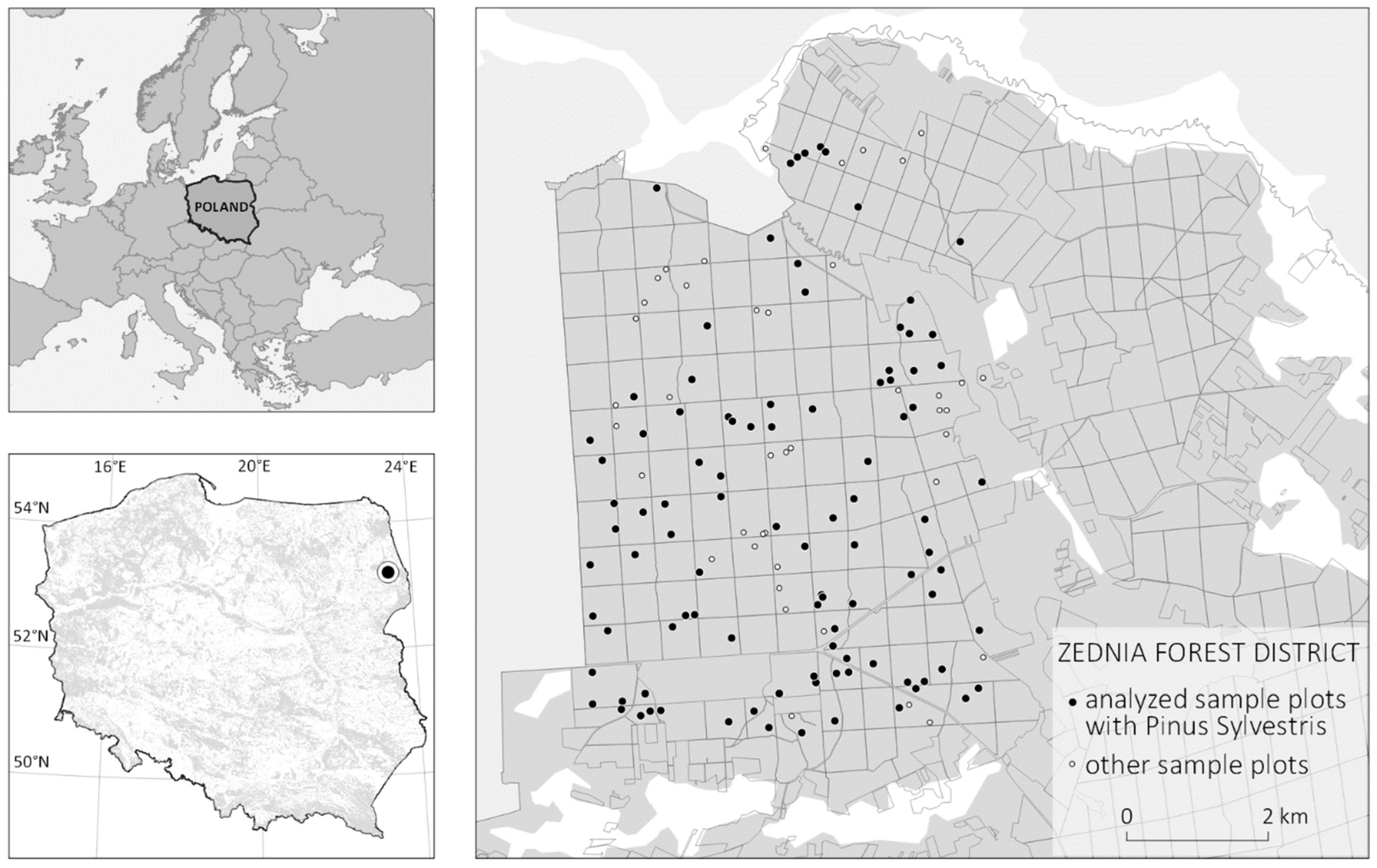
2.1. Study Area

As of the end of 2019, 29.6% of Poland, located in Central Europe, was covered with forest [24]. State Forests (SF) govern over 75% of the forested areas. Over 65% of the forest stands in Poland are coniferous. Our experiment was carried out on a selected fragment of the Zajma forest district in the Zednia forest inspectorate, located in north-eastern Poland and within the range of the Regional Directorate of SF in Bialystok (Figure 1). The research area is located within the range of a large forest complex of the Knyszyn Forest, which constitutes more than half of the area of the forest district, in particular it covers a total area of 51 km2. Knyszynska Primeval Forest is located in the lowlands of Northeastern Poland. In this area, there are forest stands of various status: economic and protected forests, nature reserves, and Natura 2000 sites [25], which means temporary or permanent exclusion from management and submission to natural processes. In 2016, a part of the studied stands was damaged by a hurricane, which significantly disrupted the forest structure but adds value to the experiment. The choice of the study area is also supported by its coverage by other research projects, involving the acquisition and analysis of ALS data and very extensive ground surveys: the two-phase research project Zajma I and II in the Zednia Forest Inspectorate-140 circular sample plots (SPs) [26,27]. Circular SPs are the current standard in Poland for sampling the tree stands parameters (e.g., tree height, DBH, etc.) [28].

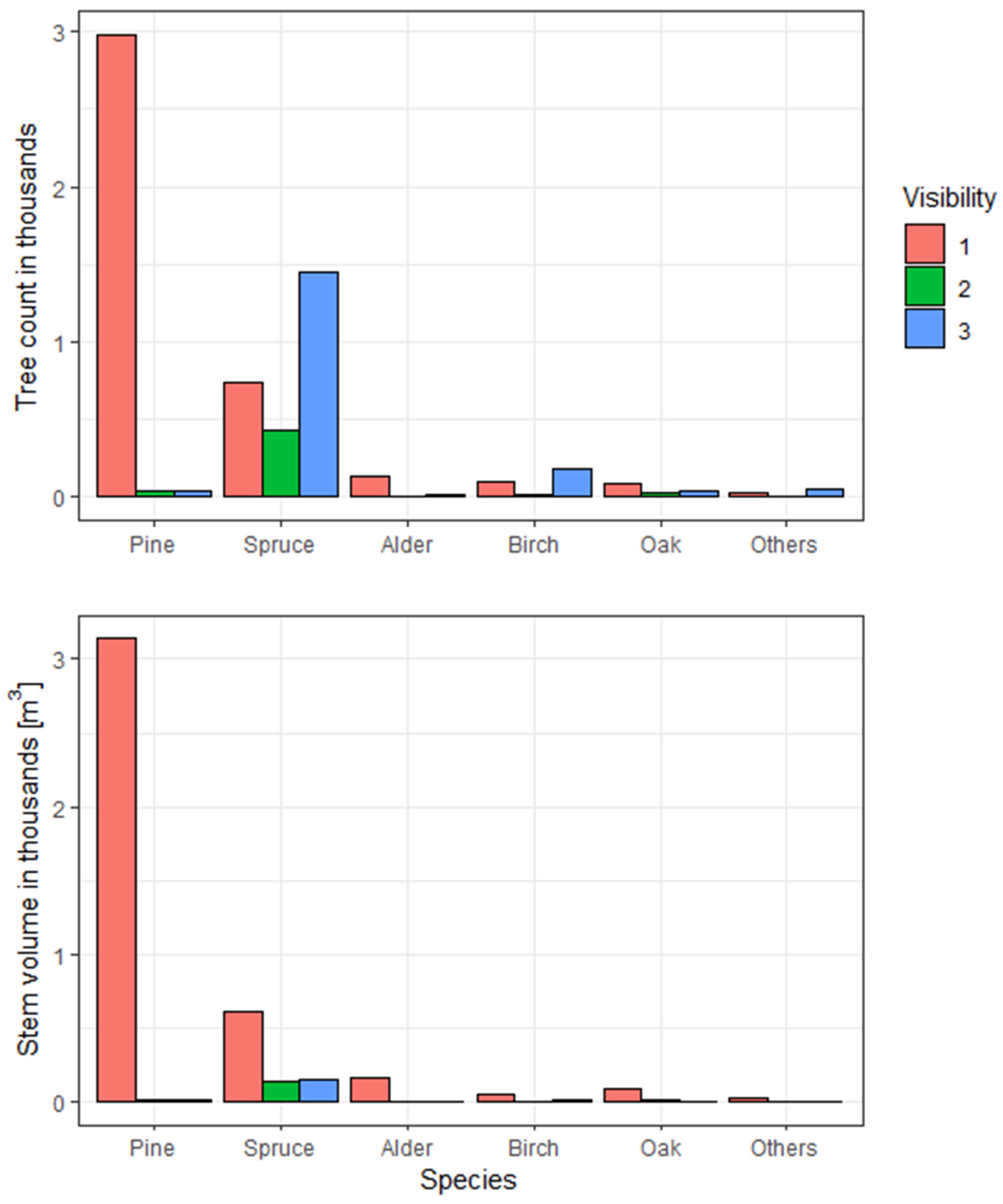
2.2. Field Inventory Data

In this study, we used data from dendrometric measurements on ground-based circular plots, which were part of a two-stage research project implemented by Forest Management and Geodesy Bureau and State Forests in 2007 (stage I) and continued in 2017 (stage II). One of the aims of this project was to assess the usability of remote sensing data acquired using passive and active techniques to determine selected parameters of trees and stands, including top height and stand abundance.
In the first phase of this project, a total of 52 SPs with radii in the 20–25 m range were established. After 10 years, dendrometric surveys were repeated on 38 of the 52 circular plots (14 plots ceased to function due to management treatments and the 2016 hurricane, which locally affected stands in the forest concession under analysis). Additionally, 102 new circular SPs were established with radii ranging from 5.64 to 12.62 m (depending on stand age class). The centers of each SP were measured with a static-mode geodetic-class Global Navigation Satellite System (GNSS) Trimble SPS 882 (mean position error = 0.41 m). The measurements for the Zajma I and Zajma II experiments were obtained from January to March of 2018. The features of each SP were determined, including sample plot location, tree count in each SP (with diameter at the breast height (DBH) greater than 70 mm), and so forth. For each tree in an SP, dendrometric features were gathered, along with the tree’s location (measurement in polar coordinates relative to the center of the sample plot), species of the tree, DBH [mm], tree height [m], crown visibility in terms of remote sensing (1—full; 2—partial; 3—no crown visibility), and additional features (sharing common crown, high trunk deflection, etc.) [29].
For the analyses, we considered the most plentiful species group in the study area, Scots pine (Pinus sylvestris L.), whose count (after rejection of disturbed observations) was estimated at 2594 individuals, ranging in age between 26 and 129 (as in 2007). It is worth noting that we included in the analyses only trees with visible tops (classes 1 and 2 according to the methodology adopted in field measurements) from a remote sensing point of view. Such an assumption was dictated by the need to be able to separate and possibly correct the contour of the crown segment of a single tree on the canopy height model (CHM). We chose pines for the analyses (except the most numerous representation) also due to the fact that pine, as a light-abundant species, practically does not occur as a canopy tree (apex visibility 3), which gives a basis to conclude that the study did not omit a significant part of the population of the studied species (Figure 2). Additionally, each tree has a digital segment outline verified both situationally and geometrically according to the adopted methodology [21].
In the context of the analyzed stands, it can be concluded that the main understory species is spruce, which constitutes almost 84% of the volume of the understory trees of the lower story (Figure 2).
For each of the analyzed Scots pine locations, we made an expert assessment of forest site affiliation based on digital terrain model (DTM) analysis (and derived products including relief variability, such as multidirectional shading maps, TPI—Topographic Position Index, etc.) and field soil and forest site work conducted in the Zednia Forest District in 2016 by staff of local division of the Bureau for Forest Management and Geodesy in Bialystok [30] based on the microrelief (local habitat conditions) matched to DTM. Microrelief affects local water and nutrient cycling and tree growth conditions [31]. Scots pine individuals were then classified into three forest site categories, forest sites groups (FSG), characterized by different trophicity levels:
(a)
HCfs—hydrogenic coniferous forest sites;
(b)
MCfs—mineral coniferous forest sites;
(c)
MMfs—mineral mixed forest sites.
Among the indicated forest sites categories, the largest sample consists of pines classified as MCfs (1761 individuals), followed by MMfs (449 individuals), while the rest belonged to HCfs (384 individuals).

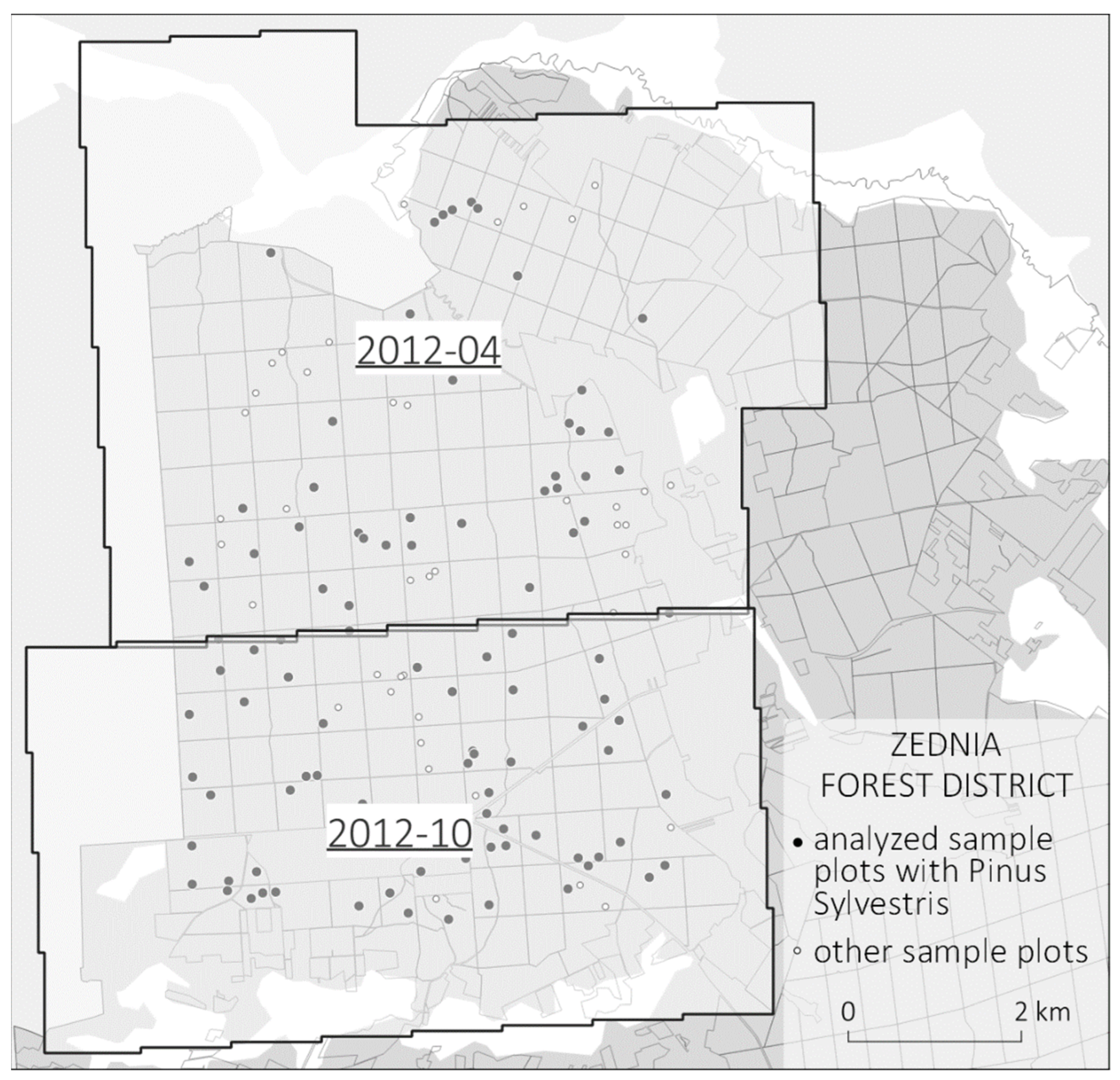
2.3. Airborne Laser Scanning Point Clouds

We used ALS point clouds acquired in years 2007, 2012, and 2017 to analyze the rate of height growth in Scots pine.
The oldest data set comes from scanning in August 2007. It has been acquired using an Optech ALTM 3100 pulsed scanner mounted on a Cessna 404 aircraft, with a flight altitude of 700 m and a speed of 120 knots (approximately 222 km/h). The ground spot diameter was approximately 0.15 m. Up to a total of four reflections were recorded, and each reflection was characterized by a reflection intensity record. The point cloud was recorded in LAS 1.0 format and was not classified. A Vexcel UltraCamX photogrammetric imaging camera was used to produce a near infrared (NIR) color orthophoto with a field resolution of 0.15 m [26].
The 2012 data set was acquired in two periods—the northern part of the study area was scanned in April 2012 and the southern part in October 2012. Figure 3 presents the distribution of circular plots, including scanning ranges from April and October 2012.
Both point clouds acquired in 2012 are a result of a country-wide project-ISOK (92% of Polish territory) aimed mainly at creating a detailed DTM for mapping potential hazards, including those related to flood risk [32,33]. Point clouds were collected using a Leica ALS70 scanner mounted on Piper PA-31 aircraft. April scanning was conducted at flight altitude of 1593–1690 m, while October scanning at 1594-1678 m. The lateral scan angles were ±16° and ±15.75°, respectively. In both cases, the flight speed was approximately 277 km/h. The footprint diameter of the laser beam on the ground surface was 0.39 m. Both data sets were aligned using TerraMatch software. For the April 2012 data, the average situational error was 0.094 m and the elevation error was 0.063 m, while for the October cloud, these were 0.070 m and 0.063 m, respectively. Point classification was performed in TerraSolid software automatically. After automatic classification, classes of points were revised manually. Points were classified according to the ASPRS standard: 1—unclassified; 2—ground; 3—low vegetation; 4—medium vegetation; 5—high vegetation; 6—buildings and engineering structures; 7—noise; 12—overlays [34]. RGB values of points in the cloud were assigned based on digital images. The resulting point cloud data set was stored in LAS 1.2 format.
The most recent data set is from August 2017 and was acquired using a Riegl LMS-Q680i scanner mounted on a Cessna 402 aircraft [27]. The flight altitude was 520 m, and the speed was 115 knots (about 213 km/h). The scan angle was 60°, and the average scan coverage was 25%. Registration was conducted in full waveform (continuous wave) mode, from which individual reflections were then extracted. RGB and color-infrared (CIR) digital color images were taken along with the scan. The CIR values were then colored with the point cloud. Additional parameters such as return number, total number of returns, scan direction and angle were also extracted. The mean error of point height mh was ≤0.15 m, while the position mp was ≤0.20 m. As with the ISOK data, the point cloud was classified according to the ASPRS standard, but class 12—overlap points—was not used. The resulting point cloud data set was stored in LAS 1.4 format.
The density parameters are as follows:
(a)
Point cloud density [pt/m2]—14.08 (2007), 8.65 (2012), 19.64 (2017);
(b)
Density of single and last returns [pt/m2] —6.84 (2007), 4.54 (2012), 4.06 (2017).

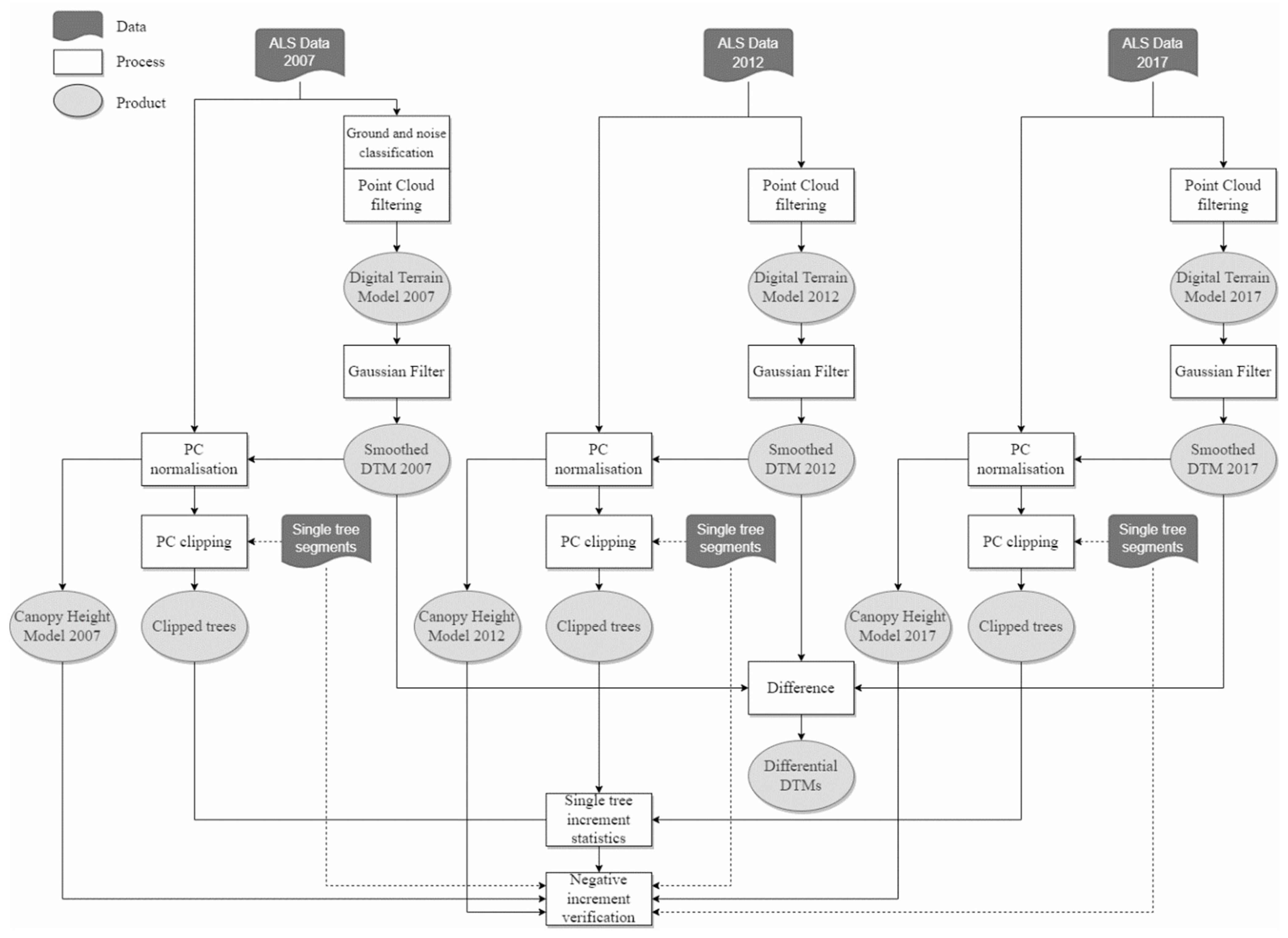
2.4. Point Clouds Processing and Derivative Products

The point clouds characterized in the previous section were used to determine the primary derived products of DTM, smoothed DTM, and CHM. DTMs on each dataset were computed using the grid_terrain algorithm and the TIN (based on a Delaunay triangulation) method derived from the lidR library [35] of the R language [36]. A pixel size of 0.5 m was assumed for each model. Class 2 and class 9 points were used when generating the DTMs, according to the ASPRS classification. For the point cloud originating in 2007, two alternative point cloud classifications were used One classification was implemented by the ALS data provider of the Zajma II experiment using the TerraScan package, the TerraSolid package, while the alternative classification was implemented using the R statistical package and the lidR package in the following two steps: (1) noise points classification (class 18 according to ASPRS standard) utilizing isolated voxels filter (IVF) method and (2) ground point classification (class 2 according to ASPRS standard) by means of progressive morphological filter (PMF) algorithm [37].
Next, we cropped DTMs to the extent of circular shape (as an orthogonal projection onto OXY plane) with a buffer size of 100 m. Then, we smoothed the cropped DTMs using a Gaussian filter derived from the SAGA GIS library [38]. Smoothing was needed to minimize the effect of classification artifacts on individual tree height calculations. The same parameters were assumed for all models: a standard deviation (sigma) of 100, a circular search window of radii of 16 pixels (equivalent to 8 m in the field-about 1.5 crowns radii of an average tree) [39].
We generated CHMs from single and first of many point cloud reflections normalized with Gaussian-filter-smoothed DTM models at 0.5 m spatial resolution and rejecting points lying below 5 m height with respect to determined terrain surface. It is worth noting that CHMs were then subjected at the post-processing stage to the process of filling in empty cells using the author’s algorithm based on pixel neighborhood analysis of the raster image, according to the methodology described in [39].

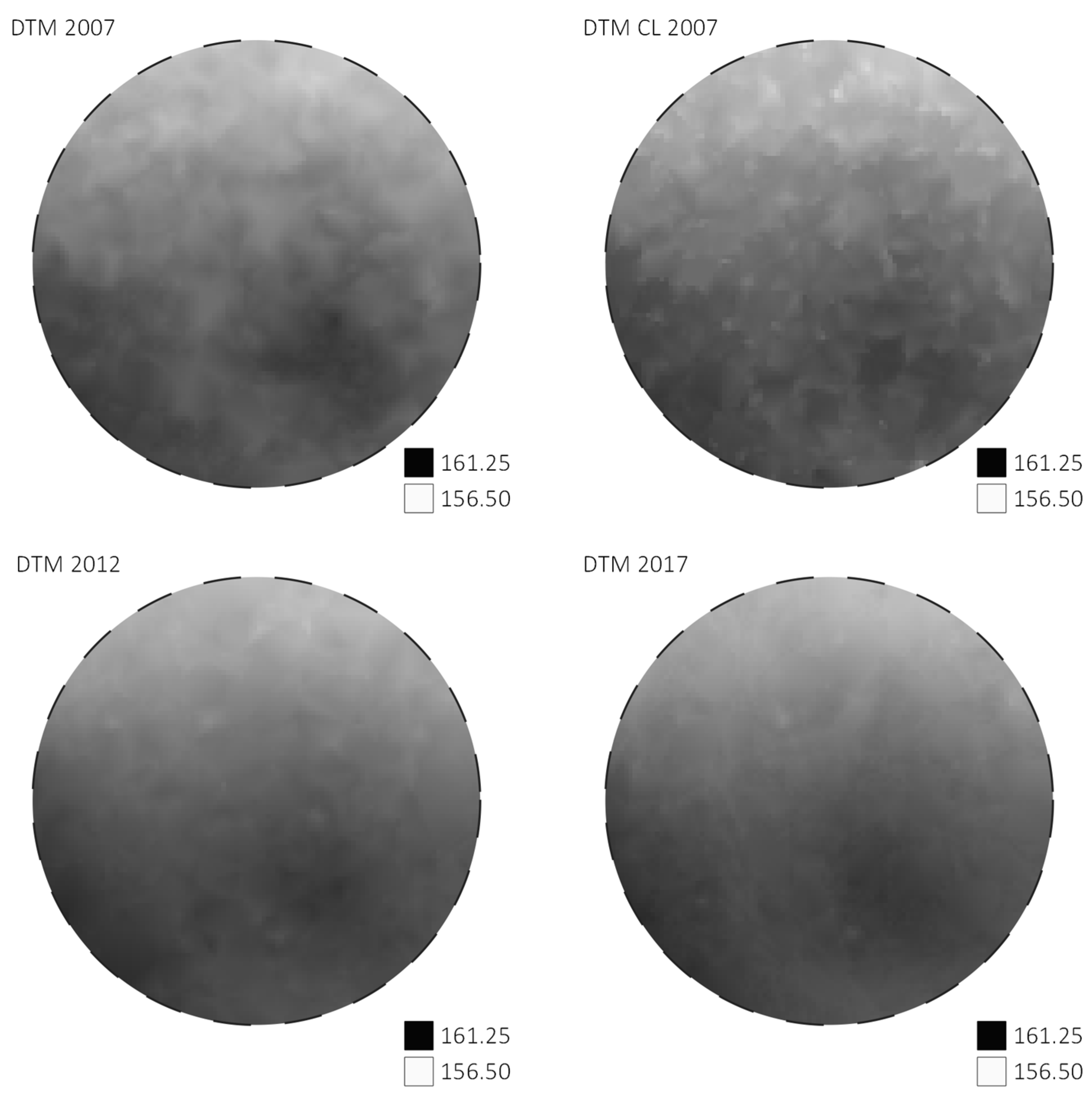
2.5. Comparative Analysis of DTM Generated from Multi-Temporal Point Clouds

In this study we made a comparative analysis of mean differences of DTMs within SPs to see if these differences are insignificant enough (with respect to tree height increment) to base calculations of relative tree heights on a single reference DTM.
The study compared four terrain models (examples in Figure 4): 2 DTMs from 2007 (DTM_CL2007—model generated based on point cloud we classified using lidR package; DTM_2007—terrain model generated using point cloud classification provided by data provider), DTM_2012 (DTM derived from ISOK point cloud), and DTM_2017 (DTM generated based on data from stage II of ZAJMA II experiment). It is worth mentioning that the 2012 DTM was generated from data acquired during the leaf-off period, while the 2007 and 2017 data were acquired during the full growing season (leaf-on).
We determined the mean values of the differences between the analyzed DTMs within each plot as zonal statistics, where the computational zone was the outline of the circular plot along with a 100 m buffer. Figure 5 shows the difference in a profile of DTMs over one of the SPs.

2.6. Tracking individual Scots Pine Height Growth

We performed the tracking of changes in the height of individual Scots pine as well as the substantive verification of the obtained results according to the procedure shown in Figure 6. First, using point clouds, we generated DTMs, which were then subjected to a smoothing process using a Gaussian filter. We used the smoothed DTMs for point cloud normalization. Point cloud normalization involves the transformation of absolute coordinates of individual points (above sea level) into relative coordinates (relative to ground level). The point cloud normalization is important in the context of obtaining information about the height of individual points relative to the terrain surface. The process of normalizing the point cloud with respect to the terrain surface was realized using the lidR library in R language.
In the next step of the adopted analytical process, we used the vector form of segments of individual trees verified situationally and geometrically based on the visual interpretation of CHM to trim the normalized point cloud using segments. It is worth mentioning that in the process of pruning the point cloud we used verified tree segments associated with the ground-based dendrometric measurements of 2017, due to the fact that within each of the analyzed segments in the studied time interval we have a set of observations. Within each segment, we performed an elevation analysis of the point cloud to determine the heights of individual trees at three time points (years 2007, 2012, and 2017). We described the heights of single individuals using three indices (measures): HTOP (height of the highest point return in the segment), HP95 (height of a point being the 95th percentile of points within analyzed segment), and HmP95 (average height of points located above HP95 within analyzed segment). Due to the fact that the height of trees was underestimated as a result of difficulty of hitting the highest point of crown with laser beam, as well as the use of ALS data with different density, our study was based on HmP95 statistics. As a result of the operation, it was possible to compare the height of each individual in consecutive reference periods separated by five-years intervals.
We observed negative height increments in a small group of cases (67 observations which constitutes 2.52% of the studied sample). Each of these cases was retrospectively analyzed using available remote sensing materials, as well as detailed data from ground-based dendrometric measurements collected during two stages of the experiment in Zajma forest area. This allowed us to identify potential reasons for this, and a detailed case studies analysis is provided in Section 3.2 and discussion section (Section 4).

2.7. Modeling of Individual Scots Pine Height Growth

In the final part of our study, we modeled the mean annual increment in a ten-year time interval (2007–2017) as a function of the height at the beginning of the study period. A frequently used function to model growth as a function of age is the Gompertz growth curve function [40,41,42,43,44]. The Gompertz curve can take different forms. In our study, we adopted its simple form:
H ( t ) = b e x p ( e x p ( a ( t c ) ) ) .
It describes the height of the tree as a function of time (age). As we are interested in the increment, i.e., the change of tree height in a time interval of constant length, therefore, to model the increment we used the derivative of Gompertz curve function, i.e., the curve of the shape described by the formula:
H ( t ) = a b e x p ( a ( t c ) e x p ( a ( t c ) ) ) .
It is important to note that the relationship we are describing is not a relationship of tree height gain dependent on time, but dependent on tree height at the beginning of the predicted measurement period of tree height change. Therefore, it is of use to predict how much the tree will grow on average each year in the next ten years. Constructing and comparing the models obtained for different habitats can be more helpful in understanding the variation in growth dynamics across habitats.
We fitted the proposed model to our data using non-linear least squares method by means of Levenberg–Marquardt algorithm implemented in the minpack.lm R package.

3. Results

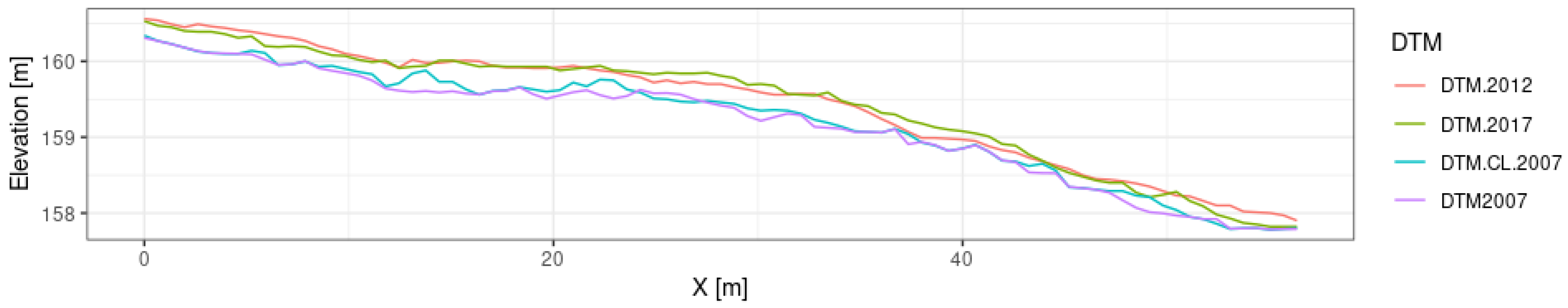
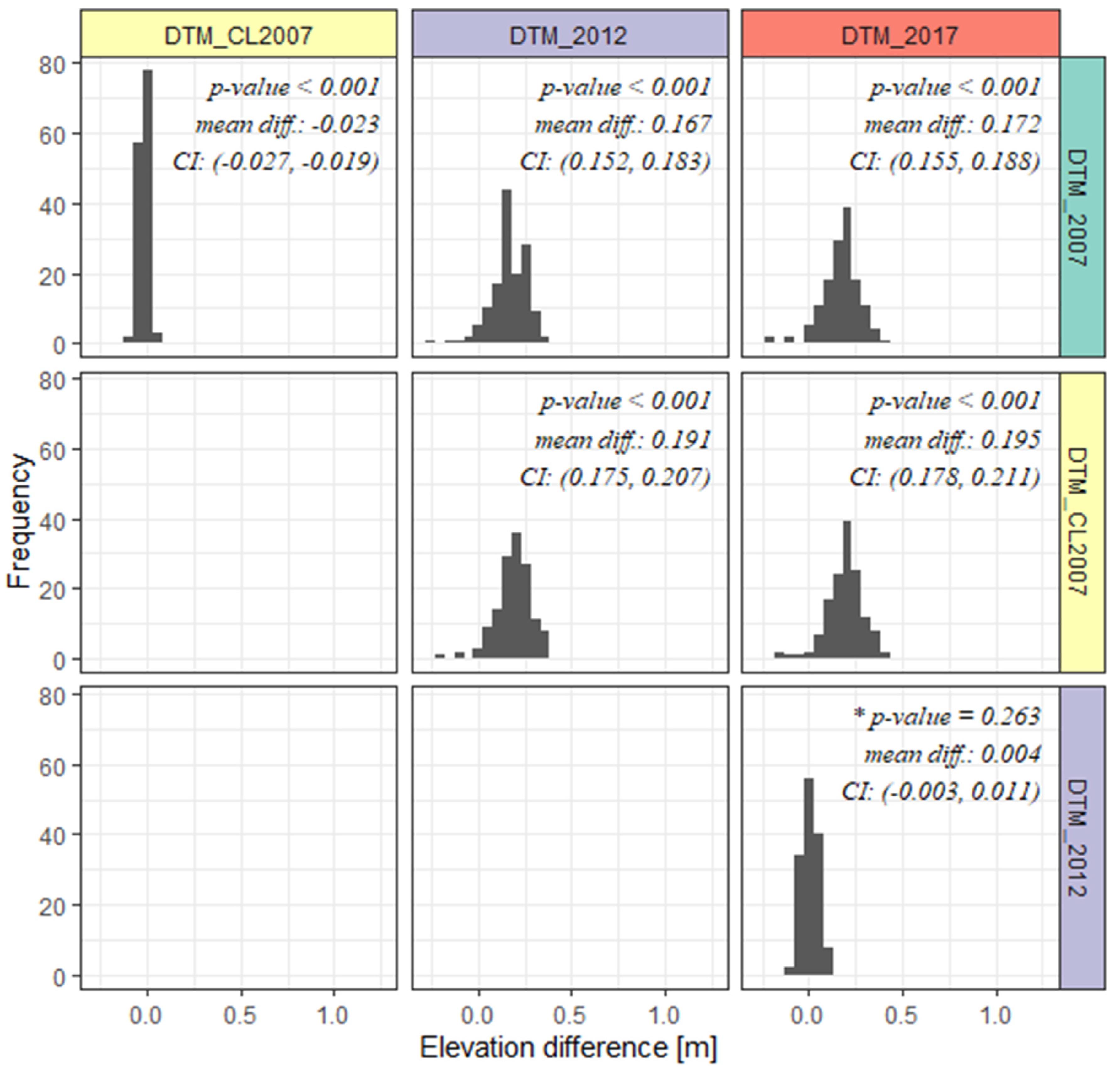
3.1. Comparative Analysis of DTMs Generated from Multi-Temporal Point Clouds

The conducted comparative analysis of mean height values in the analyzed circular plots showed the absence of statistically significant height differences between the DTMs of 2012 and 2017, where the mean height difference was indicated at the level of about 4 cm (at confidence level α = 0.05) (Figure 7). The other combinations of pairwise comparisons of DTMs models (DTM_CL2007-DTM_2012 and DTM_CL2007-DTM_2017) showed statistically significant differences in mean absolute heights, which oscillated in the range of (19,20) cm. In general, the mean height differences of the analyzed models within the SPs are relatively small, with the 2007 model being the source of the largest difference values, which could be due to the use of a sparser network of ground control points used for spatial orientation and geometric transformations of the point cloud. Very high agreement between the mean heights of the 2012 and 2017 terrain models is also evident (mean difference of 0.4 cm). The fact seems puzzling in the context of different point cloud acquisition dates. In the case of data from 2012, it was a leafless period (in accordance with the assumptions of the ISOK project), while data from the second stage of the experiment from 2017 were acquired during the leafy period (August).
Although the demonstrated differences of about 20 cm (taking into account comparative combinations of the 2007 model) seem to not be significant, this value represents nearly 83% of the mean annual growth of the tree in height, which in the initial measurement (10-year interval) had a height in the range of (20,25] m. In hydrogenic habitats, the proportion of mean differences between DTMs can, in extreme cases, even exceed 100% of the mean annual tree growth. Given these conditions, it would be unjustified to adopt one of the three models analyzed as the basis for calculating the relative height of individual trees, especially in the short time interval of the retrospective analysis (less than 5 years). However, if averages of height differences in comparative combinations of terrain models taking into account DTM from 2007 were lower, it would be reasonable to adopt the reference model generated on the basis of ALS data acquired in the leafless period, as it was assumed in main methodological assumptions of the ISOK project. The DTM obtained from the ALS during the vegetation period may be a bit higher than the one obtained based on ALS in the leafless period due to the presence of vegetation in a forest floor layer. This is one of the reasons why we have investigated the differences between DTMs, as these were based on point clouds from ALS in different seasons. As the difference was not too large compared to the possible tree height growth in the investigated period, it did not influence our analysis.
It is worth mentioning here that using two alternative classifications of ground class points on ALS data from 2007 did not result in significant differences in the mean DTM heights. The average height difference in these models was −2.3 cm.

3.2. Verification of Tree Heights 2007–2017

The availability of ALS data for the study area from three periods (2007, 2012, 2017) provides a convenient opportunity to track the growth of a large population of individuals, while allowing for additional explanatory variables such as habitat conditions of tree growth. In theory, the analyzed individuals should be characterized by positive height increment in particular research periods; nevertheless, a total of 67 cases of negative values of tree height increment (which constitutes 2.58% of the analyzed population) were recorded in the studied sample, which is associated with various factors of biotic and abiotic natures. In this paper, an attempt was made to systematize knowledge concerning potential causes of such state of affairs, which is crucial in the context of performing this type of analyses with the use of automatic methods. Among the causes of negative values of the tree height increment, one may note:
(a)
Correctness/unambiguity of top detection—the use of point clouds with different density parameters, non-uniform point distribution, or even the same data acquisition technology (impulse scanning, full-wave registration) may cause the real vertex (the highest point in the segment) to not always be correctly identified on multitemporal materials. As a consequence, this may lead to the generation of negative height increments, especially if the data acquisition interval is small (1–2 years) and the analyzed trees are characterized by low annual growth dynamics.
(b)
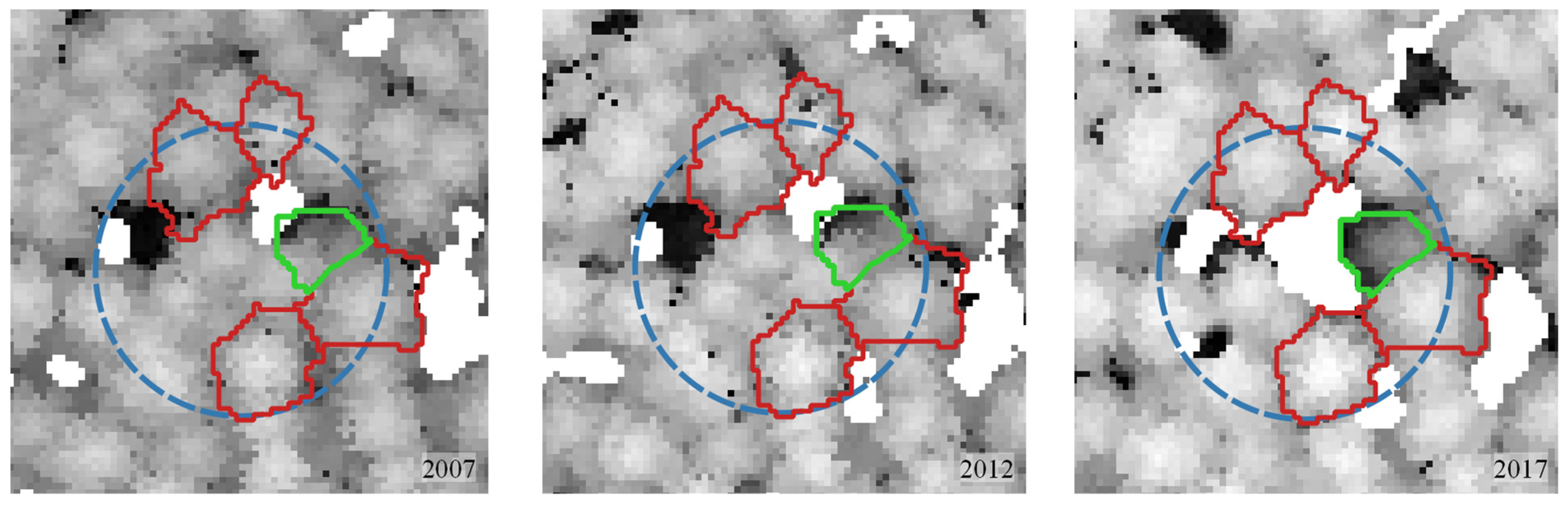
Removal of individual trees (due to management activities or natural processes)—segments developed on 2017 CHM data are used as reference data in this analysis. When a neighboring tree (that was taller) was removed of the analyzed individual, a portion of crown of the taller neighboring tree that was removed may be obscuring the analyzed segment when calculating height in previous time points (2007 and/or 2012). The situation is visualized in Figure 8.
(c)
Terminal phase of trees—Scots pine trees entering the terminal phase are characterized by the priority of growth in thickness and not in height; moreover, their tops show a tendency to bend, which, in the examined time interval, may give minimal or even negative growth in height.
(d)
Other factors disturbing the normal growth of trees—affecting an individual during the surveyed period by factors causing disease (defoliation) or dying of trees (Figure 9 and Figure 10), damage to guiding shoots due to sudden weather events.
(e)
Incorrectly determined (delineated) crown contour boundary, which results in incorrect height statistics and uncertainty in tree growth analysis.

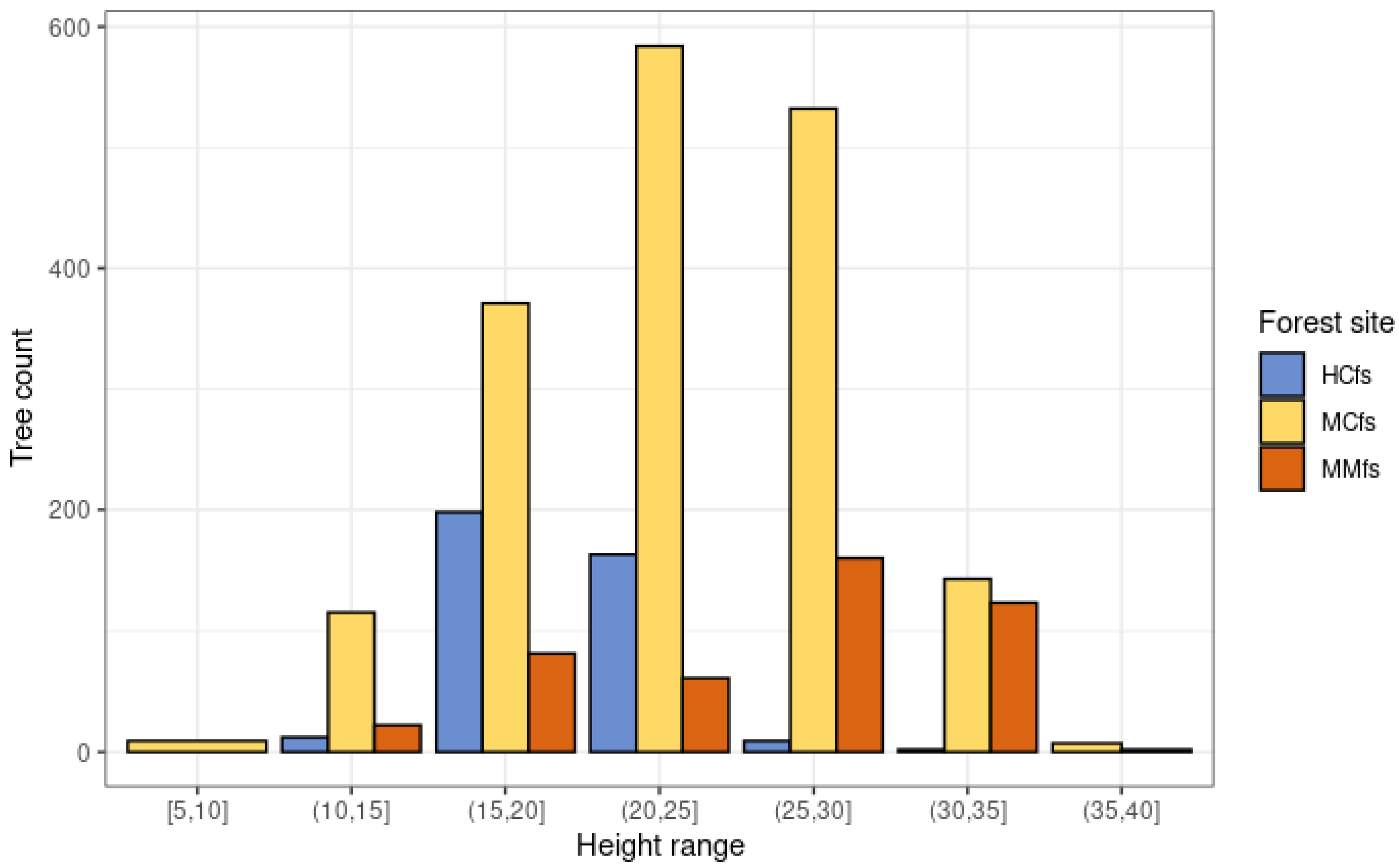
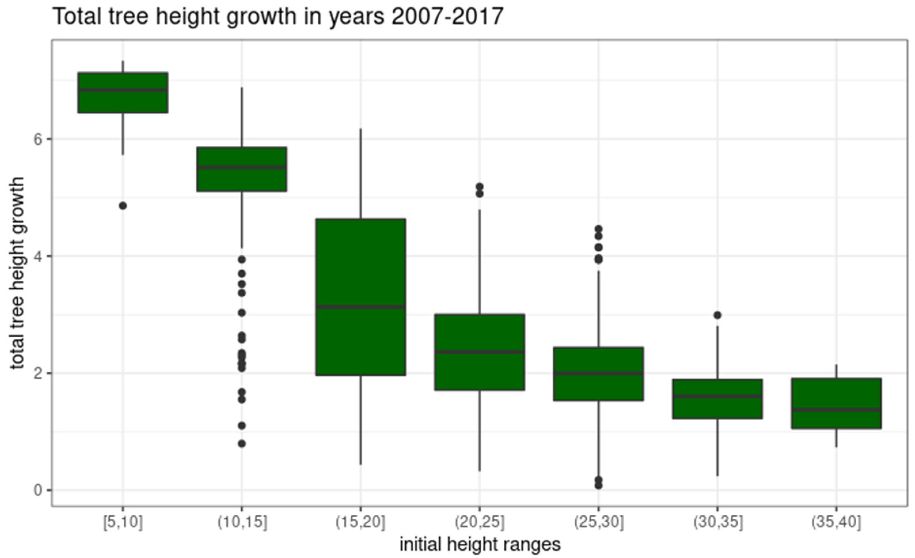
3.3. Scots Pine Height Growth Rate in 2007–2017 for the Whole Sample

We completed single-tree increment studies using 2594 Scots pine individuals, for which we determined height using ALS data from 2007, 2012, and 2017. Observations with negative changes in the tree heights in any of the study periods were not included in this analysis.
Figure 11 summarizes the sample sizes for each FSG in the tree height ranges (tree height based on HmP95 obtained from 2007 ALS data). The dominant group represented is MCfs with 1761 trees. Less abundant categories are those associated with the HCfs (384 trees) and MMfs (449 trees) groups. Trees associated with the HCfs group occur in a much smaller height range compared to the other groups due to habitat considerations (hydrogenic habitats).
Analyzing the height growth of an individual Scots pine in the study area, we observe a natural trend: as the tree is taller at the beginning of the analyzed period its change in height is smaller (Figure 12). Taking into account all observations, it can be concluded that the increment of individual Scots pine trees in the period 2007–2017 ranged from 0.08 to 7.34 m, with an average of 2.60 m. Taking into account the height variations of trees at the time of initial observation (2007), it is possible to indicate that the average increments in the heights of Scots pine in the study area range from 1.37 m for individuals in the height range of (35,40] to 6.56 m for individuals in the height range [5,10]. Disregarding the extreme ranges of initial tree height, in which the statistical sample is of a low number, it can be indicated that the average increment in Scots pine height in the studied 10-year period ranges from 1.62 m in (30,35] to 5.25 m in (10,15] initial height ranges.
Table 1 summarizes the descriptive statistics of Scots pine tree growth analyzed in initial height ranges. As can be seen from the data summarized in Table 1, the growth of individual Scots pine trees during the analyzed period are characterized by a wide range of values. This is related to additional differentiating variables. In this study, we considered forest site group as a crucial differentiating variable.

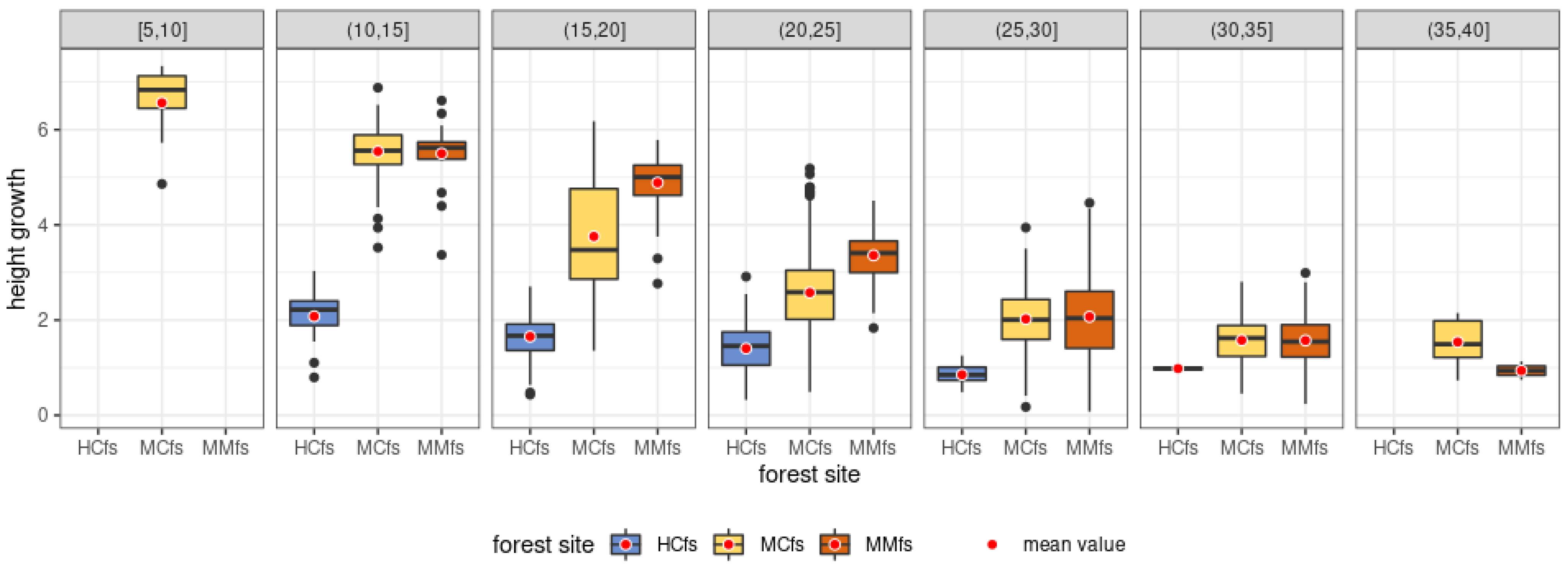
3.4. Average Scots Pine Height Growth Rate in 2007–2017 across Different Forest Site Groups

The inclusion in the analysis of the habitat conditions under which trees grew during the study 10-year period provides clear grounds for concluding that the habitat significantly determines the conditions for tree height growth [31]. In a special way, this influence is marked in relation to HCfs categories, i.e., habitats subject to permanent or periodical soil moisture (Table 2 and Figure 13).
The HCfs habitat group is characterized by a relatively small average height increment during the 10-year study period at 1.54 m (with an average for the entire set of observations of 2.60 m), as well as a small range of height increment at 2.71 m. Higher values of average tree height increment were recorded for the other habitat groups, namely, 2.79 m in the MCfs group and 2.78 m in the MMfs group, respectively.
Analyzing the average increments in the height of individual trees in particular height ranges in the 2007–2017 period, it can be concluded that, in the habitat category HCfs, the average increments range from 1.30 m (H in (10, 15]) to 0.54 m (H in (30, 35]). The average increments in the studied decade are clearly lower than in the other habitat groups (MCfs and MMfs), except for the initial height range of (30,35] m (average increment of 0.54 m), where the average 10-year increments do not differ so significantly from the other habitat categories (0.73 m—MCfs; 0.67 m—MMfs). A direct comparison of Scots pine height increments in the MCfs and MMfs sites indicates that increments during the study period remain at a relatively similar level. Nevertheless, the average increments in Scots pine in the (15, 30] m height range are slightly higher for the MMfs group by 0.51 m (in the (15, 20] m height range), by 0.47 m ((20, 25] m height range) and by only 0.08 m ((25, 30] m height range), respectively (Figure 13).

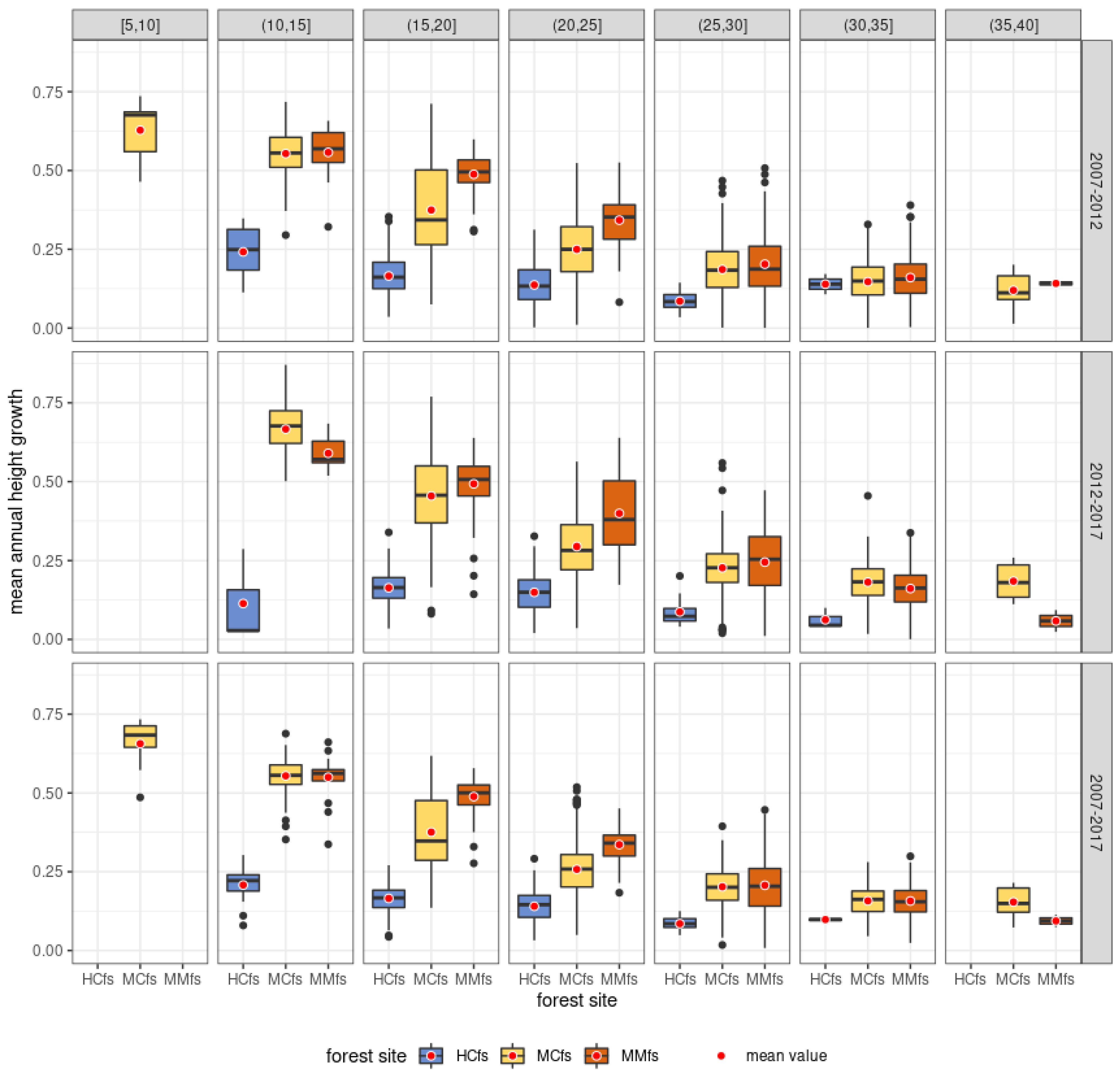
3.5. Dynamics of Annual Height Growth Rate in Time Ranges 2007–2012 and 2012–2017

Due to the variation in scanning dates in 2012 (835 observations were scanned in April 2012, while 1759 observations were scanned in October 2012), it was necessary to normalize scanning periods for each Scots pine tree analyzed in order to be able to determine precise tree growth rates. If the tree was included in the October scan, we considered that the same number of growing seasons had passed between each scan (2007–2012—five growing seasons; 2012–2017—five growing seasons). There is only a slight difference (about 1 month difference) when it comes to 2012, where the scanning from that year took place in October (i.e., after the complete cessation of annual increment in that climate zone), while the scanning from 2017 is from the second half of August (trees were in the final stage of annual increment deposition). For simplicity, we assumed in the paper that this difference would not be considered in the calculations. In the case where the tree was included in the April 2012 scan, we considered that the tree was subjected to full annual increment during four growing seasons between the 2007 and 2012 scans, while between 2012 and 2017 we assumed it was six full growing seasons. Using these values for each individual, we calculated the average annual increment between 2007 and 2012 and between 2012 and 2017.
The variability in the mean annual increment in height of Scots pine in the periods 2007–2012, 2012–2017, and 2007–2017 in individual height ranges with the consideration of habitat variability is presented in Figure 14. As can be seen from the analysis of the data in the figure below, the dynamics of the mean annual increment in height of Scots pine in the 2012–2017 period is generally higher than in the 2007–2012 period and is most noticeable for the MCfs category.

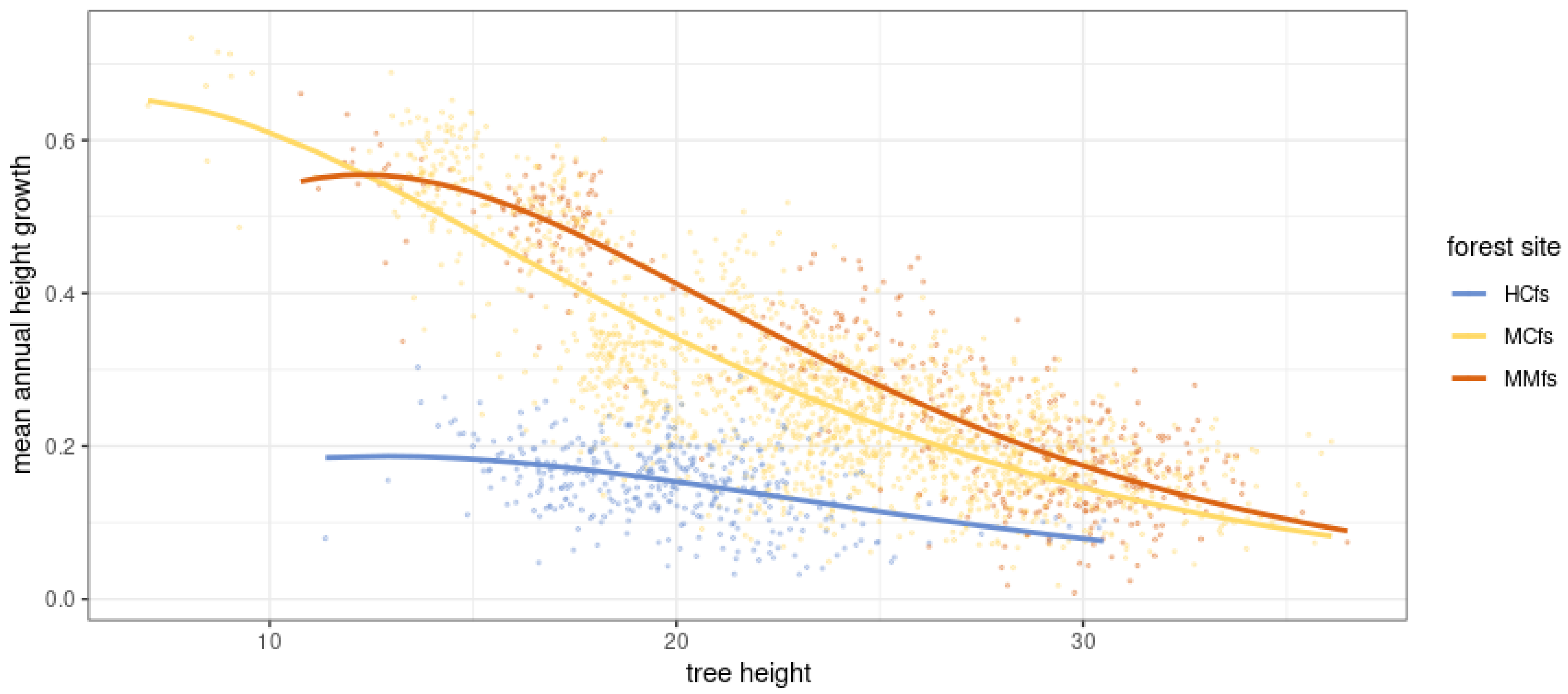
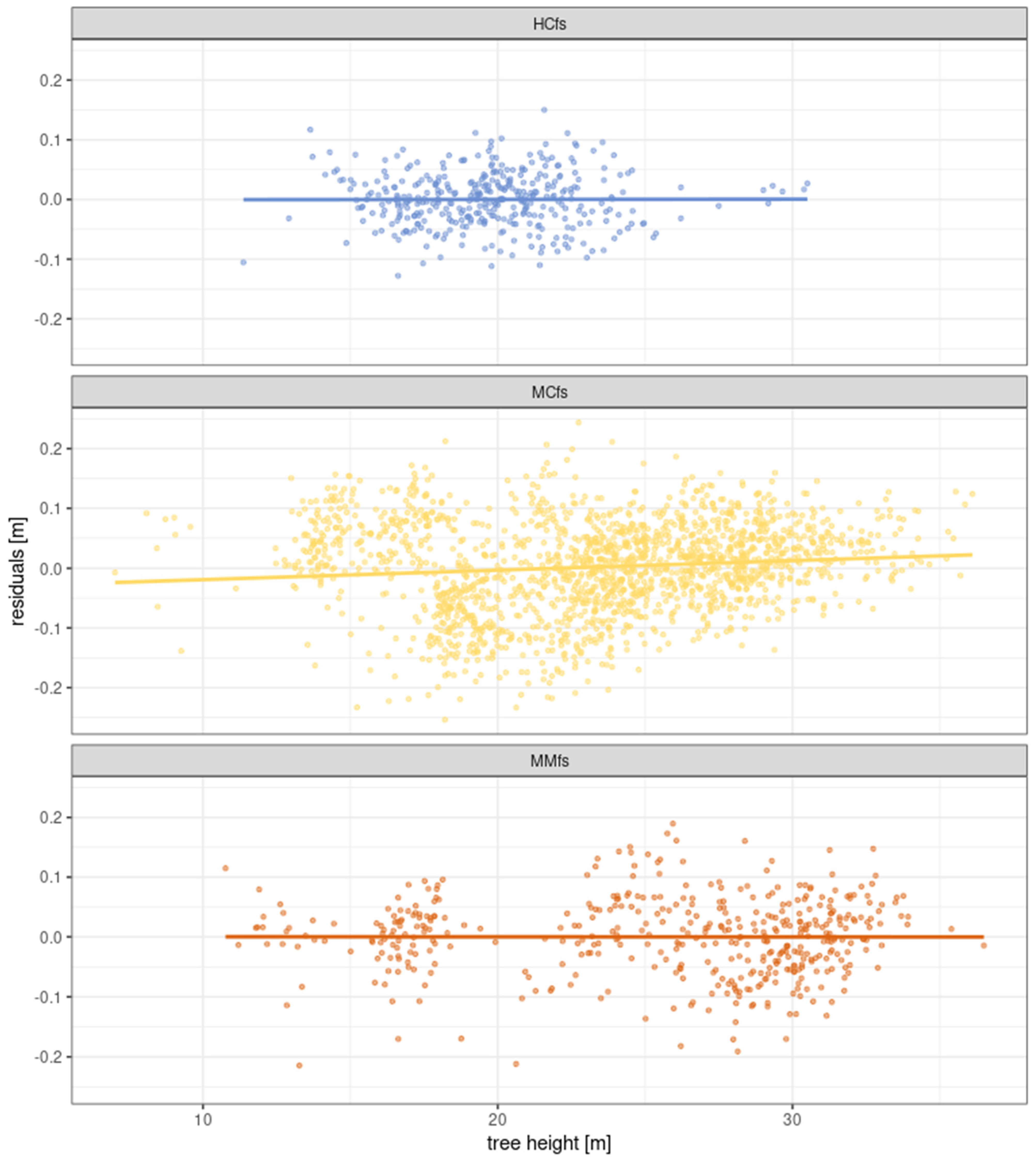
3.6. Modeling Scots Pine Height Growth including Forest Site Variability—Fitting a Gompetrz Curve

We modeled the incremental increase in pine tree height relative to its height at the beginning of the measurement period. For this purpose, we used the derivative of the Gompertz curve function. The best-fit Gompertz function curves can be found in Figure 15. Table 3 shows the parameters of the fitted functions and the fit indices.
Figure 16 shows the residuals from the fitted curves. Residuals for MCfs is slightly dependent on the tree height-the trend line has non-zero slope parameter. For MMfs, the trend line of residuals given the initial tree height has a near-zero slope line.
Figure 17 shows the models in a broader domain of tree height starting from H = 0.

4. Discussion

The aim of this study was to investigate the variability in the height increment in single Scots pine trees taking into account information on forest site productivity. In the study, we made an attempt to move away from using the age variable to tree height in the modeling process. Until now, tree age along with stand top height has been used to construct growth curves for species and determine site productivity. In our work, we propose to replace age with upper height since age is a relatively difficult parameter to measure due to the time-consuming and labor-intensive nature of the measurement or even ecological aspects (local damage as a result of the Pressler auger causing the risk of local depreciation of the wood material). Additionally, the precise tree age determination is difficult because of the semi-natural character of the study area (Knyszynska primeval forest), where the majority of individual trees come from natural regeneration. Therefore, it may result in trees of completely different ages growing next to each other. This trend will be further exacerbated by increasing conservation requirements and pressure to increase the naturalness of the forest.
Unlike tree age, it is entirely different from the tree height parameter, which in the light of widespread availability of data collected using active remote sensing techniques, together with methods of analysis of these data, allows for precise determination of this parameter at the level of a single individual. In this context, there is a clear advantage of remote technologies over field measurement of tree height, even though there are some limitations, such as the difficulty of correctly estimating the height of understory trees with ALS technology or the difficulty of identifying tops when using terrestrial laser scanning (TLS) data [19,45].
The proposed approach based on point cloud analysis within single trees (tree segments) also has limitations. The first is the possibility of negative tree increments during the study period, which, as our study indicates, may be due to biotic and abiotic causes. Tracking individual tree height increments will furthermore depend on the effectiveness of ALS data analysis methods, particularly single tree detection. Many studies are devoted to evaluating the effectiveness of crown contour delimitation methods from CHM or point cloud directly depending on the nature of analyzed stands (age, species mixing, type of use) [27,29,46,47,48].
In this type of analysis, the parameters of multitemporal data are significant. The fact that the temporal analysis is often conducted with the use of materials differing in basic technical parameters constitutes a limitation. In the case of ALS data, there may be a problem with differences in scanning technology (pulse scanner, full-waveform type) or in point cloud density. Differences in density increase the uncertainty associated with the correct determination of the maximum height within a segment. In this paper, we proposed to determine the single height as a statistic of the average height from points above the 95th percentile. While this approach may result in a systematic underestimation of the maximum height, it increases the robustness of the method to artificially inflating the height when a point from a segment of a neighboring, much higher tree is found within the reference segment. It is possible when the identified highest point is close to the tree segment boundary. Figure 18 compares the horizontal excursions from the centroid of the segment of the highest reflection in the segment and the averaged point above the 95th percentile of height. This graph shows that the highest reflection is often more skewed from the segment centroid than the accepted averaged point. There are studies that show scanning density does not influence the precision of individual tree height measurement much [49]. We did not analyze the influence of the variability of the scanning angle on individual tree height measurement precision. Although, according to [50], a scanning angle up to 30° has a minor influence on measuring the height of individual trees.
The analysis of the data showed that in most cases, the mean annual height growths of Scots pine were characterized by higher dynamics in the period 2012–2017 compared to the reference period 2007–2012. The theoretical reason for this could be an underestimation of the height of individual trees determined on the point cloud of 2012 due to lower density compared to the products of 2007 and 2017 or the influence of other factors, the variability of which was not analyzed in this study, including meteorological conditions (precipitation distribution, temperature).
The presented results showed the local effect of site productivity on the variation of height growth of single Scots pine trees. This trend was particularly marked within the HCfs category. The elaboration of curves of tree height increment in relation to initial height has a significant practical value, especially in the context of height updating in areas where no up-to-date ALS data are available and where such data are used for the inventory of forest resources. In order to construct such curves, it is necessary to provide information on the productivity of the habitat and the height of trees [51,52]. For example, in the forest areas in Poland under the management of PGL LP periodically (with an interval of about 20 years), soil-habitat works are carried out, providing a number of data on the natural diversity of habitats and vegetation occurring there [28]. The situation is similar when it comes to the wide availability of the ALS data, among others, due to the realization of national projects such as ISOK orother scientific and research projects or works connected with typical forest resources inventory.
The curves fitted to the data of average annual increment over the study period 2007–2017 relative to initial tree height in the study period provide a reasonably good approximation of the relationship between these variables in the height domain under the study. We construct these relationships under the assumption that tree height varies according to the Gompertz curve from 0 up to some fixed maximum height. The fitted functions show the differences between Scots pine trees found in different habitats. In particular, functions fitted to Scots pine trees growing in HCfs and MMfs habitats can be used to predict stand height growth in the following years without knowing their age, which, unlike height, is a difficult parameter to measure.
Analysis of residuals from fitted curves and problems with model fitting for MCfs habitat indicate that we need to search for the indicated relationship on a wider sample of trees enriched with more trees of lower height (H < 15 m). In the future, we can also look for other factors to build models that influence the explanatory variable. One such variable appearing in the literature could be the density of forest cover in the vicinity of the measured tree or the method of forest management [4].

5. Conclusions

In this study, we presented a method for utilizing multitemporal ALS data acquired in 2007, 2012, and 2017 to track the height of 2594 Scots pine trees. The results show the strong influence of habitat conditions on the increment in Scots pine. The development of local tree growth models as a function of initial height offers the possibility of their practical use in the tree height updating and growth prediction of Scots pine in other areas with similar habitat conditions.
As a result of our work, we attempted to systematize knowledge on the factors that interfere with conducting this type of analysis, which included multi-temporal data parameters (acquisition date, point cloud density), as well as other abiotic and biotic factors. The paper also proposes an approach for determining tree height in a reference segment in the form of an average height of points above the 95th percentile of tree height as a method more resistant to height fluctuations and data quality variability. In our opinion, conducting continuous experiments on individual tree height growth changes from multitemporal ALS data combined with forest site productivity is one of the key elements of the idea of precision forestry.

Author Contributions

Conceptualization, M.K. (Marek Ksepko) and Ł.K.; methodology, M.K. (Marek Ksepko), Ł.K., S.C. and M.K. (Marcin Kozniewski); software, M.K. (Marcin Kozniewski); validation, M.K. (Marek Ksepko), Ł.K., S.C. and M.K. (Marcin Kozniewski); formal analysis, M.K. (Marcin Kozniewski); investigation, Ł.K., S.C. and M.K. (Marcin Kozniewski); resources, S.C.; data curation, S.C. and M.K. (Marcin Kozniewski); writing—original draft preparation, Ł.K. and S.C.; writing—review and editing, M.K. (Marek Ksepko) and M.K. (Marcin Kozniewski); visualization, S.C. and M.K. (Marcin Kozniewski); supervision, M.K. (Marek Ksepko) and Ł.K.; project administration, M.K. (Marek Ksepko); funding acquisition, M.K. (Marek Ksepko). All authors have read and agreed to the published version of the manuscript.

Funding

The APC was covered by Bialystok University of Technology under the Grants WZ/WI-IIT/3/2020 and WZ/WB-INL/3/2021 funded by Ministry of Science and Higher Education.

Data Availability Statement

Not applicable.

Conflicts of Interest

The authors declare no conflict of interest.

References

  1. Jiang, Z.D.; Owens, P.R.; Ashworth, A.J.; Fuentes, B.A.; Thomas, A.L.; Sauer, T.J.; Wang, Q.B. Evaluating tree growth factors into species-specific functional soil maps for improved agroforestry system efficiency. Agrofor. Syst. 2022, 96, 479–490. [Google Scholar] [CrossRef]
  2. Hynynen, J.; Repola, J.; Mielikäinen, K. The effects of species mixture on the growth and yield of mid-rotation mixed stands of Scots pine and silver birch. For. Ecol. Manag. 2011, 262, 1174–1183. [Google Scholar] [CrossRef]
  3. Borowski, M. Przyrost Drzew I Drzewostanow; Panstwowe Wydawnictwo Rolnicze i Lesne: Warszawa, Poland, 1974. [Google Scholar]
  4. Gizachew, B.; Brunner, A. Density-growth relationships in thinned and unthinned Norway spruce and Scots pine stands in Norway. Scand. J. For. Res. 2011, 26, 543–554. [Google Scholar] [CrossRef]
  5. Rudnicki, M.; Silins, U.; Lieffers, V.J. Crown cover is correlated with relative density, tree slenderness, and tree height in lodgepole pine. For. Sci. 2004, 50, 356–363. [Google Scholar]
  6. Pretzsch, H. Canopy space filling and tree crown morphology in mixed-species stands compared with monocultures. For. Ecol. Manag. 2014, 327, 251–264. [Google Scholar] [CrossRef]
  7. Sibona, E.; Vitali, A.; Meloni, F.; Caffo, L.; Dotta, A.; Lingua, E.; Motta, R.; Garbarino, M. Direct measurement of tree height provides different results on the assessment of LiDAR accuracy. Forests 2016, 8, 7. [Google Scholar] [CrossRef]
  8. Fardusi, M.J.; Chianucci, F.; Barbati, A. Concept to practice of geospatial-information tools to assist forest management and planning under precision forestry framework: A review. Ann. Silvic. Res. 2017, 41, 3–14. [Google Scholar]
  9. Wunder, J.; Brzeziecki, B.; Żybura, H.; Reineking, B.; Bigler, C.; Bugmann, H. Growth-mortality relationships as indicators of life-history strategies: A comparison of nine tree species in unmanaged European forests. Oikos 2008, 117, 815–828. [Google Scholar] [CrossRef]
  10. Zhen, Z.; Quackenbush, L.J.; Zhang, L. Trends in automatic individual tree crown detection and delineation—Evolution of LiDAR data. Remote Sens. 2016, 8, 333. [Google Scholar] [CrossRef]
  11. Moskal, L.M.; Erdody, T.; Kato, A.; Richardson, J.; Zheng, G.; Briggs, D. Lidar applications in precision forestry. In Proceedings of the Silvilaser 2009, College Station, TX, USA, 14–16 October 2009; pp. 154–163. [Google Scholar]
  12. Goodbody, T.R.; Coops, N.C.; Marshall, P.L.; Tompalski, P.; Crawford, P. Unmanned aerial systems for precision forest inventory purposes: A review and case study. For. Chron. 2017, 93, 71–81. [Google Scholar] [CrossRef]
  13. Instytut Badawczy Leśnictwa (Forest Research Institute). Remote Sensing Based Assessment of Woody Biomass and Carbon Storage in Forests (RemBioFor). 2015. Available online: http://rembiofor.pl/en/305-2/ (accessed on 1 May 2022).
  14. Instytut Badawczy Leśnictwa (Forest Research Institute). Comprehensive Monitoring of Stand Dynamics in Białowieża Forest Supported with Remote Sensing Techniques (ForBioSensing). 2014. Available online: http://www.forbiosensing.pl/about-project (accessed on 1 May 2022).
  15. Tymińska-Czabańska, L.; Hawryło, P.; Socha, J. Assessment of the effect of stand density on the height growth of Scots pine using repeated ALS data. Int. J. Appl. Earth Obs. Geoinf. 2022, 108, 102763. [Google Scholar] [CrossRef]
  16. Zawieja, B.; Kazmierczak, K. Longitudinal analysis of annual height increment differentiation in Scots pine (Pinus sylvestris L.) stands of different age classes. Folia For. Polonica. Ser. A For. 2014, 56, 179–184. [Google Scholar] [CrossRef] [Green Version]
  17. Yu, X.; Hyyppä, J.; Kaartinen, H.; Hyyppä, H.; Maltamo, M.; Rönnholm, P. Measuring the growth of individual trees using multi-temporal airborne laser scanning point clouds. In Proceedings of the ISPRS Workshop Laser Scanning, Enschede, The Netherlands, 12–14 September 2005; Volume 2005, pp. 204–208. [Google Scholar]
  18. Ma, Q.; Su, Y.; Tao, S.; Guo, Q. Quantifying individual tree growth and tree competition using bi-temporal airborne laser scanning data: A case study in the Sierra Nevada Mountains, California. Int. J. Digit. Earth 2018, 11, 485–503. [Google Scholar] [CrossRef]
  19. Wang, Y.; Lehtomäki, M.; Liang, X.; Pyörälä, J.; Kukko, A.; Jaakkola, A.; Liu, J.; Feng, Z.; Chen, R.; Hyyppä, J. Is field-measured tree height as reliable as believed—A comparison study of tree height estimates from field measurement, airborne laser scanning and terrestrial laser scanning in a boreal forest. ISPRS J. Photogramm. Remote Sens. 2019, 147, 132–145. [Google Scholar] [CrossRef]
  20. Loehle, C.; Solarik, K.A. Forest growth trends in Canada. For. Chron. 2019, 95, 183–195. [Google Scholar] [CrossRef]
  21. Kazmierczak, K. The current growth increment of pine tree stands comprising three different age classes. Leśne Pr. Badaw. 2013, 74, 93. [Google Scholar] [CrossRef]
  22. Arumäe, T.; Lang, M.; Laarmann, D. Thinning-and tree-growth-caused changes in canopy cover and stand height and their estimation using low-density bitemporal airborne lidar measurements–a case study in hemi-boreal forests. Eur. J. Remote Sens. 2020, 53, 113–123. [Google Scholar] [CrossRef]
  23. Kamińska, A.; Lisiewicz, M.; Stereńczak, K. Single Tree Classification Using Multi-Temporal ALS Data and CIR Imagery in Mixed Old-Growth Forest in Poland. Remote Sens. 2021, 13, 5101. [Google Scholar] [CrossRef]
  24. Zajączkowski, G.; Jabłoński, M.; Jabłoński, T.; Szmidla, H.; Kowalska, A.; Małachowska, J.; Piwnicki, J. Raport o Stanie Lasów W Polsce 2019 [Report on the State of Forests in Poland 2019]; Centrum Informacyjne Lasów Państwowych: Warsaw, Poland, 2020. [Google Scholar]
  25. Evans, D. Building the European Union’s Natura 2000 network. Nat. Conserv. 2012, 1, 11–26. [Google Scholar] [CrossRef]
  26. Gajko, K.; Myszkowski, M.; Ksepko, M. Eksperyment w obrębie Zajma. Geod. Mag. Geoinformacyjny 2009, 1, 60–62. [Google Scholar]
  27. Kolendo, Ł.; Ksepko, M. Selection of optimal tree top detection parameters in a context of effective forest management. Ekonomia i Środowisko 2019, 68, 67–85. [Google Scholar]
  28. Dyrekcja Generalna Lasów Państwowych (General Directorate of the State Forests). Instrukcja Urządzania Lasu. Część II [Instruction for Forest Management. Part II]; Ośrodek Rozwojowo-Wdrożeniowy Lasów Państwowych: Bedoń, Poland, 2012. [Google Scholar]
  29. Stereńczak, K.; Kraszewski, B.; Mielcarek, M.; Piasecka, Ż.; Lisiewicz, M.; Heurich, M. Mapping individual trees with airborne laser scanning data in an European lowland forest using a self-calibration algorithm. Int. J. Appl. Earth Obs. Geoinf. 2020, 93, 102191. [Google Scholar] [CrossRef]
  30. BULiGL. Operat Glebowo-Siedliskowy dla Obszaru Nadleśnictwa Żednia. In Soil and Forest Site Survey for the Żednia Forest District; 2018; Unpublished Report. [Google Scholar]
  31. Vanguelova, E.I.; Nortcliff, S.; Moffat, A.J.; Kennedy, F. Morphology, biomass and nutrient status of fine roots of Scots pine (Pinus sylvestris) as influenced by seasonal fluctuations in soil moisture and soil solution chemistry. Plant Soil 2005, 270, 233–247. [Google Scholar] [CrossRef]
  32. Wężyk, P. Podręcznik dla uczestników szkoleń z wykorzystania produktów LiDAR. In The Handbook for LiDAR Data Utilization Training; Główny Urząd Geodezji i Kartografii: Warsaw, Poland, 2014. [Google Scholar]
  33. Państwowe Gospodarstwo Wodne Wody Polskie Informatyczny System Ochrony Kraju. 2009. Available online: https://isok.gov.pl/o-projekcie.html (accessed on 2 June 2022).
  34. American Society for Photogrammetry and Remote Sensing. LAS Specification. Version 1.2. 2008. Available online: https://www.asprs.org/wp-content/uploads/2010/12/asprs_las_format_v12.pdf (accessed on 1 February 2022).
  35. Roussel, J.R.; Auty, D.; Coops, N.C.; Tompalski, P.; Goodbody, T.R.; Meador, A.S.; Bourdon, J.F.; de Boissieu, F.; Achim, A. lidR: An R package for analysis of Airborne Laser Scanning (ALS) data. Remote Sens. Environ. 2020, 251, 112061. [Google Scholar] [CrossRef]
  36. R Core Team. R: A Language and Environment for Statistical Computing; R Foundation for Statistical Computing: Vienna, Austria, 2020. [Google Scholar]
  37. Zhang, K.; Chen, S.C.; Whitman, D.; Shyu, M.L.; Yan, J.; Zhang, C. A progressive morphological filter for removing nonground measurements from airborne LIDAR data. IEEE Trans. Geosci. Remote Sens. 2003, 41, 872–882. [Google Scholar] [CrossRef]
  38. Conrad, O.; Bechtel, B.; Bock, M.; Dietrich, H.; Fischer, E.; Gerlitz, L.; Wehberg, J.; Wichmann, V.; Böhner, J. System for automated geoscientific analyses (SAGA) v. 2.1. 4. Geosci. Model Dev. 2015, 8, 1991–2007. [Google Scholar] [CrossRef]
  39. Kolendo, Ł.; Kozniewski, M.; Ksepko, M.; Chmur, S.; Neroj, B. Parameterization of the Individual Tree Detection Method Using Large Dataset from Ground Sample Plots and Airborne Laser Scanning for Stands Inventory in Coniferous Forest. Remote Sens. 2021, 13, 2753. [Google Scholar] [CrossRef]
  40. Miklewska, J. Including the growth function into the renewable resources optimal control models. Folia Universitatis Agriculturae Stetinensis. Oeconomica 2007, 48, 233–242. [Google Scholar]
  41. Jarosz, K.; Klapec, B. Modelowanie wzrostu drzewostanow z wykorzystaniem funkcji Gompertza. Sylwan 2002, 146, 35–42. [Google Scholar]
  42. El-Gohary, A.; Alshamrani, A.; Al-Otaibi, A.N. The generalized Gompertz distribution. Appl. Math. Model. 2013, 37, 13–24. [Google Scholar] [CrossRef]
  43. Hanusz, Z.; Siarkowski, Z.; Ostrowski, K. Zastosowanie modelu Gompertz’a w inżynierii rolniczej. Inżynieria Rol. 2008, 12, 71–77. [Google Scholar]
  44. Rymuza, K.; Bombik, A.; Radzka, E. Zastosowanie wybranych nieliniowych modeli do opisu wzrostu rutwicy wschodniej (Galega orientalis Lam.). Acta Agrophysica 2018, 25, 373–383. [Google Scholar] [CrossRef]
  45. Mielcarek, M.; Kamińska, A.; Stereńczak, K. Digital Aerial Photogrammetry (DAP) and Airborne Laser Scanning (ALS) as Sources of Information about Tree Height: Comparisons of the Accuracy of Remote Sensing Methods for Tree Height Estimation. Remote Sens. 2020, 12, 1808. [Google Scholar] [CrossRef]
  46. Sačkov, I.; Hlasny, T.; Bucha, T.; Juriš, M. Integration of tree allometry rules to treetops detection and tree crowns delineation using airborne lidar data. Iforest-Biogeosciences For. 2017, 10, 459–467. [Google Scholar] [CrossRef]
  47. Lisiewicz, M.; Kamińska, A.; Stereńczak, K. Recognition of specified errors of Individual Tree Detection methods based on Canopy Height Model. Remote Sens. Appl.: Soc. Environ. 2022, 25, 100690. [Google Scholar] [CrossRef]
  48. Lisiewicz, M.; Kamińska, A.; Kraszewski, B.; Stereńczak, K. Correcting the Results of CHM-Based Individual Tree Detection Algorithms to Improve Their Accuracy and Reliability. Remote Sens. 2022, 14, 1822. [Google Scholar] [CrossRef]
  49. Van Lier, O.R.; Luther, J.E.; White, J.C.; Fournier, R.A.; Côté, J. Effect of scan angle on ALS metrics and area-based predictions of forest attributes for balsam fir dominated stands. Forestry 2022, 95, 49–72. [Google Scholar] [CrossRef]
  50. Keränen, J.; Maltamo, M.; Packalen, P. Effect of flying altitude, scanning angle and scanning mode on the accuracy of ALS based forest inventory. Int. J. Appl. Earth Obs. Geoinf. 2016, 52, 349–360. [Google Scholar] [CrossRef]
  51. Socha, J.; Solberg, S.; Tymińska-Czabańska, L.; Tompalski, P.; Vallet, P. Height growth rate of Scots pine in Central Europe increased by 29% between 1900 and 2000 due to changes in site productivity. For. Ecol. Manag. 2021, 490, 119102. [Google Scholar] [CrossRef]
  52. Socha, J.; Tymińska-Czabańska, L.; Bronisz, K.; Zięba, S.; Hawryło, P. Regional height growth models for Scots pine in Poland. Sci. Rep. 2021, 11, 10330. [Google Scholar] [CrossRef]
Figure 1. The study area is located in Northeastern Poland (Central Europe). The bottom left map presents territory of Poland with the distribution of forested areas in gray and the marked location of Zednia Forest District. The map on the right presents the ground sample plots which are distributed across the Zednia Forest District.
Remotesensing 14 04170 g001
Figure 2. Comparison of field tree count of each species in the analyzed stands distinguishing by their visibility in the context of stem volume.
Remotesensing 14 04170 g002
Figure 3. Spatial distribution of SPs with partition into aerial laser scanning dates in 2012: April scanning and October scanning.
Remotesensing 14 04170 g003
Figure 4. An example of 4 versions of digital terrain models (DTM) for the same circular sample plot (SP).
Remotesensing 14 04170 g004
Figure 5. Comparison of profiles of the digital terrain models (DTMs) covering the same circular sample plot.
Remotesensing 14 04170 g005
Figure 6. ALS data processing procedure for obtaining height measurements of individual Scots pine trees from each of the three scannings and verification of the tree height increment values.
Remotesensing 14 04170 g006
Figure 7. Comparison of distributions of mean elevation differences on smoothed terrain models generated based on 2007, 2012, and 2017 ALS data. * statistically significant.
Remotesensing 14 04170 g007
Figure 8. Example of a circular sample plot (blue, dashed outline) over time. Consequence of removing a tree obscuring the crown of a lower tree (green outline) between 2012 and 2017 on the calculation of increments within reference segments. Measurement of the tree height of the other neighboring Scot Pine trees (red outline) were not influenced by this process.
Remotesensing 14 04170 g008
Figure 9. Examples of trees with negative height increment in the period 2007–2017: left—due to terminal stage and tip bending, right—due to tree dying.
Remotesensing 14 04170 g009
Figure 10. Example of a circular sample plot (blue, dashed outline) over time. We observe here a gradual death of a tree (green outline) and consequent reduction in the extent of its canopy area. Other Scot Pine trees (red outline) were not affected by this process.
Remotesensing 14 04170 g010
Figure 11. The count of Scots pine trees in tree height ranges (wysokość na podstawie HmP95 i danych ALS z 2007 roku) across different forest site groups: hydrogenic coniferous forest sites (HCfs), mineral forest sites (Mfs), mineral mixed forest sites (MMfs).
Remotesensing 14 04170 g011
Figure 12. Distributions of ten years (2007–2017) of height growth of Scots pine trees in different initial height ranges.
Remotesensing 14 04170 g012
Figure 13. Distributions of ten years (2007–2017) of height growth of Scots pine trees across different forest site groups: hydrogenic coniferous forest sites (HCfs), mineral forest sites (MMfs), mineral mixed forest sites (MMfs).
Remotesensing 14 04170 g013
Figure 14. Distributions of mean annual height increments for Scots pine in the 2007–2012, 2012–2017, and 2007–2017 height ranges with habitat variation.
Remotesensing 14 04170 g014
Figure 15. Incremental and elevation models of Scots pine including habitat variation against measurements. Fitted curves represent derivatives of the function describing the Gompetrz curve.
Remotesensing 14 04170 g015
Figure 16. Residuals from the fitted function related to Gompetrz curve, an approximation of annual tree height growth based on initial tree height along with linear regression with least squares method. Slight dependence of residuals for model of Scot pines on MCfs can be noticed.
Remotesensing 14 04170 g016
Figure 17. Comparison of the fitted growth functions based on Gompetrz growth curve, an approximation of annual tree height growth based on initial tree height.
Remotesensing 14 04170 g017
Figure 18. Horizontal deviations from the centroid of the segment of the highest reflection in the segment and averaged point above the 95th percentile of points’ height. The deviation is defined as the ratio of the distance between the centroid and the analyzed point and the pseudo-diameter of the tree crown-the diameter calculated from the segment area assuming circularity of the segment’s shape. The shaded area represents the distance of the point from the centroid of the segment by 0.8 pseudo-radius (0.4 pseudo-diameter).
Remotesensing 14 04170 g018
Table 1. Descriptive statistics of ten years (2007–2017) of height growth of Scots pine trees in different initial height ranges.
Height Range [m]MinP5P25MedianMeanP75P95MaxCount
5–104.865.216.456.846.567.137.267.349
10–150.802.445.135.475.255.816.306.88129
15–200.481.251.983.303.394.825.586.37606
20–250.320.941.702.362.423.053.996.01770
25–300.180.991.612.082.112.583.244.46711
30–350.080.731.271.621.621.952.533.14353
35–400.730.741.061.141.371.912.082.1516
sum2594
Table 2. Descriptive statistics of ten years (2007–2017) of height growth of Scots pine trees across different forest site groups: hydrogenic coniferous forest sites (HCfs), mineral forest sites (Mfs), mineral mixed forest sites (MMfs).
Forest Site GroupMinP5P25MedianMeanP75P95MaxCount
HCfs0.320.661.211.561.541.852.313.03384
MCfs0.181.151.872.522.793.315.537.341761
MMfs0.080.851.542.362.783.915.426.61449
sum2594
Table 3. The parameters and statistics of fitted Gompertz function to model the growth of the height for a given initial tree height. Statistically significant parameters of the function are in bold (p-value < 0.05).
Forest Site GroupabcR2adj. R2MAERMSE
HCfs−0.09725.224312.79750.16210.15540.03560.0450
MCfs−0.073339815−32.28560.67570.67520.05930.0745
MCfs (bounded)−0.100617.71326.00000.66440.66380.06090.0760
MMfs−0.114313.201412.27310.81360.81240.05030.0647
Publisher’s Note: MDPI stays neutral with regard to jurisdictional claims in published maps and institutional affiliations.

