
Generation of Combined Daily Satellite-Based Precipitation Products over Bolivia


Centro de Investigaciones en Ingeniería Civil y Ambiental, Universidad Privada Boliviana, Cochabamba 3967 UPB, Bolivia
*
Author to whom correspondence should be addressed.
Remote Sens. 2022, 14(17), 4195; https://doi.org/10.3390/rs14174195
Submission received: 20 July 2022
/
Revised: 15 August 2022
/
Accepted: 17 August 2022
/
Published: 26 August 2022
(This article belongs to the Special Issue Remote Sensing for Precipitation Retrievals)
Abstract
:This study proposes using Satellite-Based Precipitation (SBP) products and local rain gauge data to generate information on the daily precipitation product over Bolivia. The selected SBP products used were the Global Satellite Mapping of Precipitation Gauge, v6 (GSMaP_Gauge v6) and the Climate Hazards Group Infrared Precipitations with Stations (CHIRPS). The Gridded Meteorological Ensemble Tool (GMET) is a generated precipitation product that was used as a control for the newly generated products. The correlation coefficients for raw data from SBP products were found to be between 0.58 and 0.60 when using a daily temporal scale. The applied methodology iterates correction factors for each sub-basin, taking advantage of surface measurements from the national rain gauge network. Five iterations showed stability in the convergence of data values. The generated daily products showed correlation coefficients between 0.87 and 0.98 when using rain gauge data as a control, while GMET showed correlation coefficients of around 0.89 and 0.95. The best results were found in the Altiplano and La Plata sub-basins. The database generated in this study can be used for several daily hydrological applications for Bolivia, including storm analysis and extreme event analysis. Finally, a case study in the Rocha River basin was carried out using the daily generated precipitation product. This was used to force a hydrological model to establish the outcome of simulated daily river discharge. Finally, we recommend the usage of these daily generated precipitation products for a wide spectrum of hydrological applications, using different models to support decision-making.
1. Introduction
One of the most important variables in hydrological models is precipitation data, which allows models to be grouped according to their manner of using data. Models can be classified as either semi-distributed [1] or distributed [2], and the precipitation data used as the input for the hydrological models can be monthly, daily and hourly. Monthly data is utilized in historical analyses of precipitation [3,4] and climate change analyses [5]. Hourly data can be used for extreme event analysis [6,7,8] and storm analysis. Daily precipitation data can be employed in all these applications: historical analysis [9], climate change analysis [10,11], extreme event analysis [12,13] and storm analysis.
All precipitation data sets can be obtained using the same methods, which can be either direct or indirect. Direct methods employ rain gauges and meteorological stations as measurement instruments and are considered to be more accurate than indirect methods. Examples of their successful use include gathering data on variations in the amount, frequency and intensity of precipitation along the western coastline of Sumatra [14]; improving gridded precipitation data sets, based on radar-detected precipitation, and validating these with rain gauges in regions in Israel and the Netherlands [15], analyzing rain gauge quantification of the Ganges River basin in India [16] and generating climate indices in Brazil [17]. However, these direct method instruments also raise certain concerns. These include density issues, as seen in the Ebro River basin in Spain [18], rain gauge operation and design issues [19] and climate and altitude factors [20]. Indirect methods are, therefore, useful as substitutes.
When discussing indirect methods, it is worth considering how satellite sensors and radar instrumentation capture precipitation data. The generation process for satellite sensors results in satellite-based precipitation (SBP) products. These provide the most accessible radar-generated precipitation data and have been employed in various studies [21,22]. Popular precipitation products include the global satellite mapping of precipitation (GSMaP) [23,24] and the Climate Hazards Group Infrared Precipitations with Stations (CHIRPS) [25,26]. CHIRPS has been used to evaluate extreme precipitation in the Qinghai-Tibet Plateau, China [27] and the Brazilian Amazon [28], while GSMaP has been used for precipitation analysis in the mountainous regions of Nepal [29] and Iran [30]. Despite their accessibility and ease of handling, SBP products have several issues that require further consideration.
One such issue is that SBP products are constantly updated through the introduction of new versions and products, and analysis is required to understand variations in these updates. An example is the Climate Hazards Group, which had its main product—the Climate Hazards Group Infrared Precipitations (CHIRP)—before it added stations to the algorithm and developed CHIRPS [31]. IMERG precipitation products provide another example. Three versions of the same product were issued—early, late and final—the main difference between them being the processing time [32]. In contrast, SBP products show “estimated precipitation”, which does not represent precipitation registers on the ground. The utilization of SBP products requires the analysis of SBP (see case studies of the Mekong River basin [33] and a segment of the Nile River in Egypt [34]) and the employment of a methodology (for example, bias correction) to rectify the precipitation data before it can be used in another research [35,36].
Another consideration is that experience with SBP products, such as rain gauges, highlights the challenges of using these products in studies. The generation of combined precipitation products using both SBP and rain gauge data can offer an alternative that improves information accuracy and generates a distributed precipitation product. One study in China used a deep neural network fusion model between convolutional neural networks (CNN) and a long–short-term memory network (LSTM) with daily temporal resolution. This study employed TRMM 3B42 V7 satellite data, rain gauge data, and thermal infrared images for the release of the fusion [37]. The “three-cornered hat” (TCH) is another merging method that employs an inverse error variance-covariance matrix to estimate uncertainty and generate weighted precipitation data for SBP products. The TCH method requires at least three data sets to be employed, using either daily or monthly temporal resolution [38]. Another combined method involves using an optimized methodology base for the entropy, variance and standard deviation for daily precipitation data. This methodology, which was applied in the Chaobai River in China, utilizes PERSIANN-CCS [39].
Our focal country, Bolivia, has around 381 rain gauges with 36 years of precipitation data [40]. Nonetheless, rain gauge density does not exist in the ranges recommended by the World Meteorological Organization (WMO) [41]. In light of this, Bolivia’s Ministry of Environment and Water (known by its Spanish acronym, MMAyA) requested the integration of generated precipitation products for use in its Balance Hídrico Superficial de Bolivia (BHSB) [40]. The result of this request was the implementation of a gridded meteorological ensemble tool (GMET) product [42]. However, generating this product requires high-end computing equipment, which limits its ability to be replicated in other case studies. Moreover, it employs a combined method that utilizes the relative error and a number of iterations to generate a monthly precipitation product for Bolivia [43].
The objective of this study is to generate a combined daily precipitation data set for Bolivia. The SBP products selected are GSMaP and CHIRPS.
2. Materials and Methods
2.1. Study Area
Bolivia is a landlocked country in the central region of South America, with an area of 1,098,006 km2 and elevations varying between 200 m and 5000 m above sea level (m.a.s.l.). The country’s range of elevations has resulted in three distinct ecological regions: the highlands, valleys and lowlands. The focal areas for this study are Bolivia’s three major river basins.
The first, the Altiplano basin, is located in the southwest of the country between 66°5′W and 69°44′W longitude and between 14°35′S and 22°96′S latitude. With an area of 151,722 km2, this endorheic basin is considered to be Bolivia’s smallest major basin. It encompasses primarily the highland ecological region (Figure 1a), and its elevation ranges between 3500 and 5000 m.a.s.l. Figure 1b shows an elevation profile of the main river connecting Lake Titicaca with Lake Poopó. In this profile, the elevation difference around these lakes is approximately 750 meters.
Bolivia’s second major basin, the Amazon, is located in the central, northern and northeastern parts of the country, between 59°39′ and 69°40′W longitude and between 9°36′S and 20°32′S latitude. With an area of 720,792 km2, it is the largest basin in this study (Figure 1a). The Amazon basin, which discharges into the Atlantic Ocean, encompasses the three previously mentioned ecological regions. As seen in Figure 1c, the elevation difference between the source of the main river and the point where it exits Bolivia is around 4100 meters.
The third major basin, the La Plata, is located in the south and southeast of the country, between 57°23′ and 67°2′W longitude and 16°10′S and 22°55′S latitude, with an area of 225,492 km2. It discharges into the Atlantic Ocean and encompasses the three previously mentioned ecological regions (Figure 1a). The elevation difference of the La Plata basin is similar to that of the Amazon basin and can be observed along the length of the main river (Figure 1d).
Figure 2 contains annual precipitation and temperature maps for Bolivia for the period 2001–2015. The Altiplano basin shows precipitation intensities varying between 200 mm and 750 mm per year and temperatures between −4 °C and 5 °C. In the Amazon basin, mean precipitation is around 500 mm to 3000 mm per year and the mean temperature is between 4 °C and 28 °C. The La Plata basin has mean precipitation of around 400 mm to 2300 mm per year, with temperatures varying between −4 °C and 25 °C. It is clear from these figures that precipitation and temperature in Bolivia are directly related to the country’s ecological regions.
2.2. Data Set
The satellite-based products GSMaP_Gauge v6 and CHIRPS were used to generate monthly combined precipitation products. GSMaP is an SBP product developed by the Japan Aerospace Exploration Agency (JAXA). It has a spatial resolution of 0.1° (approximately 10 km) and hourly temporal resolution [23,24]. CHIRPS is an SBP product that was developed at the Climate Hazards Center of the University of California, Santa Barbara. This product has a spatial resolution of 0.05° (approximately 5 km) and three different temporal resolutions (daily, pentadal and monthly) [25,26].
The gridded meteorological ensemble tool (GMET) generates gridded precipitation and temperature data through spatially correlated, random fields (SCRFs) sampled from the standard normal distribution [44]. This method requires precipitation and temperature data from the rain gauge. The GMET employs an ensemble method to generate gridded maps. The final map is the result of merging the generated gridded maps. The GMET can generate gridded maps with different pixel sizes. In the case of Bolivia and the BHSB, because of the low density of rain gauges, synthetic stations had to be generated using CHIRPS precipitation data [30] gathered between 1980 and 2016. The final gridded spatial resolution was about 0.05°.
For this study, all precipitation data (SBP products, GMET and rain gauge maps) require a spatial resolution of 0.05°.
2.3. Development Method
The iterative combined method is based on the adjustment of relative error between rain gauge data and SBP product data. Before proceeding to a discussion of this method, several considerations must be highlighted.
2.3.1. Sub-Basins Map
This methodology employs a sub-basins system following the national sub-division. To start the process, a sub-basin map must be defined.
The sub-basin map employed in the previous study was the official Pfafstetter Level Three coding system for Bolivia [43]. This map identifies 61 sub-basins for the country. However, many of these sub-basins are not considered to be relevant due to their extensions. Therefore, in the present study, another sub-basin map was utilized. The official Pfafstetter Level Four coding system identifies 329 sub-basins. Moreover, it includes the 17 prioritized strategic basins for the Plan Nacional de Cuencas (PNC) for the period 2013–2020 [45,46]. Figure 3a shows both sub-basin systems. Some of the prioritized sub-basins are shaped for many sub-basins of Level Four, while others are for the same basins and one group is not included in the Level Four map.
After combining both maps in a shapefile (Figure 3a), it was necessary to rasterize the map to define the number of pixels comprising each sub-basin. In this process, some sub-basins were integrated into others because these have reduced areas in relation to the number of pixels. This map should have the same resolution as the precipitation maps (0.05 × 0.05°). In Figure 3b, the rasterized map presents only 296 sub-basins; it was then processed to combine the SBP products with rain gauge data.
2.3.2. Rain Gauge Data
The first step is an analysis of rain gauge data. Base data from the BHSB was depurated and filled to generate the GMET [40]. To generate the rain gauge gridded maps, kriging interpolation with a pixel size of 0.05° was used. Nevertheless, the daily precipitation data implies the existence of days on which no rain was recorded. The flow chart in Figure 4 shows the considerations applied in this case and analyzes the sum of all daily rain gauge data. If the sum was equal to zero, it was necessary to generate a precipitation map containing only one value (for the implementation of relative error). In this study, these maps contain the value of 0.1 mm per day.
In those cases when the sum was higher than zero, kriging interpolation was utilized. As a result, precipitation maps could generate negative values. In Figure 5a, the precipitation kriging map presents pixels with negative precipitation data. Because of this, it is necessary to correct the precipitation maps, assuming that all negative precipitation is equal to zero. The results can be seen in Figure 5b.
2.3.3. Rain Gauge Data
To initiate the combined method, it was first necessary to determine the relative error (RE) between rain gauge data and data from SBP products. However, Equation (1) was conditioned to the value that the rain gauges might be presented; it was necessary to add a conditional in case the rain gauge value data was zero (Equation (2)).
After determining the RE between rain gauges and SBP products, it was necessary to calculate the RE value per sub-basin. To do this, the sub-basin map was introduced to obtain maps of daily average precipitation. It was then possible to calculate the average relative error.
The relative error calculation made it possible to analyze general differences between rain gauge data and SBP products. Due to the relative error operation, high values were observed in the tables. For these cases, the values were conditioned, based on a maximum and minimum equivalent of ±95%. This conditioning allowed for the generation of an adjustment factor and control of the iterative process. In the case of the adjustment factor, this was a correction value based on the average relative error per basin that was then applied to the next equation.
The adjustment factor was used to generate a new combined product. This factor was multiplied by the SBP product, which was then used to obtain the relative error value. Once generated, the new precipitation product was analyzed utilizing the average relative error per sub-basin. The condition to accept the generation process was based on the relative error of the new precipitation product and was found to be ±5%. With this condition, the final combined precipitation product was obtained in the fifth iteration. Figure 6 presents a flow chart of the previously explained combined processes.
3. Results
3.1. Precipitation Base
The SBP products utilized in this research (GSMaP and CHIRPS) present different daily features than the data obtained from the rain gauges. Figure 7 shows the daily precipitation maps for these products. The rain gauge map (Figure 7a) shows the highest precipitation levels to be in the Amazon basin, with an average value of 8 mm per day, while the GSMaP data (Figure 7b) shows the highest precipitation levels to be in the northwest of the Amazon basin, with values of around 6 mm to 7 mm per day. The CHIRPS data (Figure 7c) shows that the highest precipitation levels—8 mm per year—correspond to the same zone as that indicated by the rain gauge data. The CHIRPS data also shows higher precipitation levels than those shown by the rain gauge data in the northwestern zone of the Amazon basin. The Altiplano and La Plata basins do not present visible differences in the various maps.
During the initial analysis of the SBP products, none of the selected data showed a high correlation with the rain gauge data. Figure 8 shows significant variations between the Altiplano (Figure 8a), Amazon (Figure 8b) and La Plata (Figure 8c) basins. These variations permitted distinctions to be made among the maximum precipitation ranges for the three basins. The maximum precipitation levels registered were 15 mm per day, 35 mm per day and 30 mm per day for the Altiplano, Amazon and La Plata basins, respectively.
In light of these findings, statistical indicators must be used to analyze the SBP products for each major basin. In Table 1, it can be seen that GSMaP presented better indicators than CHIRPS. Data for the Altiplano basin shows higher determination (R2) and correlation (R) coefficients for both products, in comparison with the other basins. The accumulated bias, relative bias, mean absolute error (MAE) and root mean square error (NSE) of this basin shows little difference between the rain gauge and SBP products. Nash-Sutcliffe efficiency values show ranges between 0.57 and 0.76, indicating acceptable relationships between the analyzed data. The best values should be close to 1.0. In all cases, the Altiplano basin presents better values in comparison with the other basins, while GSMaP is demonstrated to have a slight advantage in comparison with CHIRPS.
In this regard, only the quantitative value is insufficient to analyze the products. Figure 9 shows the daily spatial correlation coefficient of GSMaP and CHIRPS in comparison with the rain gauge data. In the case of GSMaP (Figure 9a), the map illustrates a correlation of around 0.5 in the Altiplano and La Plata basins. The Amazon basin contains regions with minor values of 0.4. On the CHIRPS map (Figure 9b), the Altiplano and La Plata basins present values of around 0.4, while the Amazon basin presents minor values of 0.3. In general, the precipitation products with daily temporal resolution present lower values, including some regions with a maximum correlation of 0.5.
3.2. Combined Precipitation
The generation of combined products allowed for the approximation of SBP product data to rain gauge data. Figure 10b shows that the combined product of the GSMaP and rain gauge data (GS) presents approximation values in the region north and northeast of the Amazon basin on the rain gauge map (Figure 10a). However, this product data is still not comparable with precipitation data from the central part of this basin, with an observable underestimation in this region. The CH data (which is the combined product of CHIRPS and rain gauge data) in Figure 10c shares many similarities with the GS product data. Slight differences are noticeable, based on precipitation values from the rain gauge data in the basin. Finally, the GMET data (Figure 10d) present an overestimation of 8 mm per year in the Amazon basin region, while the rain gauge data show average values of 6 mm to 7 mm per year. In the northwest region of this basin, the GMET data present values of around 6 mm per year, in comparison with the 4 mm to 5 mm per year shown on the rain gauge map.
Analysis of the daily values of these products shows a significant improvement versus the initial SBP products. For the Altiplano basin, Figure 11a shows that GS and CH present a slight underestimation in comparison with the rain gauge map. The GMET presents slight variations for the rain gauge data. In Figure 11b, GS and CH display several underestimations for the Amazon basin, while GMET shows an overestimation for this basin. Finally, for the La Plata basin (Figure 10c), GS and CH present a general underestimation in comparison with rain gauge values. The GMET presents several overestimations for values of around 10 mm to 30 mm per day.
Table 2 presents interesting results for an analysis of the statistical data of these values. GS and CH demonstrate a marked improvement in comparison with initial SBP products in all basins. For the Altiplano basin, GS offers a better precipitation product than CH and GMET. With an R-value of 0.97 and an NSE of 0.98, GS exceeds the next-closest product, which is CH (with an R-value of 0.93 and NSE of 0.95). For the Amazon basin, the GS and GMET show the same R-value of 0.86. However, the NSE indicator demonstrates the superiority of the GMET (NSE = 0.95) in comparison with GS (NSE = 0.87). Another significant indicator is the accumulation bias value, with GS and CH presenting values between about 7400 mm and 8000 mm. The GMET shows a value of around 4800 mm, which is about 40% less than the values of the other products. In the La Plata basin, GS presents an R-value of 0.96 and an NSE value of 0.97 in comparison with the next-best product, CH (with values of R = 0.89 and NSE = 0.90). The accumulation bias for GS is around 2030 mm, which is almost 50% less than other values in the basin. Overall, the GMET yields low values for the La Plata basin.
The spatial correlation map highlights the differences shown in the previous table. Figure 12a shows a higher GS correlation in the Altiplano and La Plata basins, with values of around 0.8 to 0.9. For the Amazon basin, some sub-basins in the north and northeast demonstrate a high correlation. In general, this basin presents moderate correlation values of around 0.4 to 0.6. For the CH precipitation product (Figure 12b), the general correlation values in the three major basins are between 0.2 and 0.6. For the GMET product (Figure 12c), the correlation values are around 0.4 to 0.8. The highest correlation values are around zones with higher rain gauge density.
3.3. Application of Generated Precipitation Products in Hydrological Modelling
In order to check the potential application of generated daily precipitation products, a hydrological model was set up in the Rocha river basin, located in the valleys of Bolivia at 2500 m.a.s.l. using HEC-HMS software. The elevation map of the studied basin and average precipitation can be seen in the panels of Figure 13. The delineated basin area reached 3626 km2. The Rocha River basin is one of the prioritized basins in the country, due to the population density and the water resources requirements of a semi-arid region. On the other hand, landslides and flash floods have been reported due to the steep slopes channeling river discharge to the central part of the valleys. Thus, daily precipitation is required for short-event hydrological analysis.
The hydrological model was set up using land use and soil texture information. The basin was divided into 59 sub-basins [47], as can be seen in Figure 14a. The size of the smallest sub-basin was 5 km2, the largest, 169 km2 and the average, 62 km2. Most of these are micro-basins where a detailed hydrological analysis is feasible. The spatial distribution of precipitation in the Rocha River basin was checked using interpolated rain gauges, GSMaP, CHIRPS, GS (enhanced GSMaP) and CH (enhanced CHIRPS), as can be seen in Figure 14b–f, respectively. The precipitation products were accumulated from 17 to 31 January 2014, when storm events in the studied area were reported. The enhanced GS and CH products clearly show the precipitation patterns in northwest and southeast areas. However, the GS product shows closer agreement with the rain gauge pattern.
The hydrological model was forced using interpolated rain gauge, GSMaP, CHIRPS, GS, and CH precipitation products. The simulated river discharge was compared with the real data observed at Puente Cajón Station, as can be seen in panels of Figure 15. A close agreement when using the GS product with the one forced by rain gauges can be noted in Figure 15a,d.
The statistical indicators of simulated river discharge at Puente Cajón Station can be seen in Table 3. The performance of simulated discharge can be noted in those indicators using the GS precipitation product compared to a rain gauge.
4. Discussion
The daily GSMaP product data represents a general overestimation in the north and northeast of the Amazon basin, while in the south, underestimation was evident in comparison to the rain gauge map data. In terms of the daily CHIRPS product, overestimation has only been evident in the northeast of the basin; the product presents similar precipitation values in the south of this basin but shows a different distribution. In comparison with the average statistics indicator for the three major basins, GSMaP presents correlation values of around 0.58 to 0.60. The best results for this product are in the Amazon basin. With NSE values between 0.69 and 0.76, this product shows a slight approximation to rain gauge values. In comparison, CHIRPS presents correlation coefficient values of around 0.50 and 0.61, along with NSE values between 0.57 and 0.72. For this product, a better result was found in the Altiplano basin. CHIRPS presents more variation in its statistical indicators than GSMaP, while GSMaP presents higher values in its correlation coefficient map.
After application of the proposed method with iterations, the combined products of GS (the results of the GSMaP and a rain gauge) and CH (the result of CHIRPS and a rain gauge) were compared with the GMET precipitation product. The GS and CH maps showed improvements in the north and northwest of the Amazon basin. However, the maps of the southern region of this basin continued to yield underestimations. Analyzing the statistical indicators, GS and CH showed several improvements in comparison to SBP products. GS presented correlation coefficient values of around 0.86 to 0.97 and NSE values of 0.87 to 0.98. This product presented the best values in the Altiplano basin and the worst values in the Amazon basin. CH showed coefficient correlation values of around 0.83 to 0.93 and NSE values of 0.86 to 0.95. The product presented similar features to those of GS. After reviewing the spatial resolution of these products, it can be seen that GS presented better correlations in the Altiplano and La Plata basins. Data for the Amazon basin showed sub-basins with low correlation values, in comparison with the rain gauge data. CH is a product offering an acceptable improvement in comparison to its SBP product base, but it is inferior to GS and is not recommended for further research use. These findings are consistent with previous works using monthly scale products in Bolivia using three selected basins [48] and 61 sub-basins [43]. Lower performance was found in the Amazon basin compared to the Altiplano and La Plata basins.
A hydrological application was employed in a prioritized basin in the central part of Bolivia, known as the Rocha River basin, to check the ability of the daily generated products to simulate daily river discharge, in order to forecast floods. It was found that the performance of simulated flow using the GS daily product was in closer agreement with the product using a rain gauge and was much better than when using CH, CHIRPS and GSMaP products.
5. Conclusions
The iterative method proposed here for generating daily precipitation data sets in Bolivia presents an alternative for reducing the bias of SBP products and covering ungauged areas. This methodology represents a feasible way to generate new precipitation data with an acceptable spatial resolution.
The combined products GS and CH present notable improvements in comparison to the SBP products that were utilized. Initially, GSMaP and CHIRPS presented correlation values of around 0.58 and 0.60, in comparison with the rain gauges. After data set generation, the combined products (GS and CH) presented correlations of around 0.87 and 0.97, while the GMET presented values of around 0.89 and 0.95 for the three basins.
Among the products employed with the iterative method, GS displays the best results. In the Altiplano and La Plata sub-basins, the product data achieves a high degree of similarity with the rain gauge data. In the case of the Amazon sub-basins, the data from the group located to the north and northeast yielded high correlation coefficient values. However, the rest of the Amazon sub-basins presented with low correlation values, showing a general underestimation of these values.
In short, the methodology proposed here can be applied in other countries to enhance the spatial and temporal resolution of precipitation data sets. These data sets can, in turn, be utilized in hydrological applications. In order to check the quality of this ability, a case study in the Rocha River basin was carried out. The daily GS precipitation product was used to force a hydrological model. The latter was able to simulate daily river discharge and forecast flood peaks in the Rocha River basin. Therefore, we recommend the use of these daily generated precipitation products in a wide spectrum of hydrological applications, using different models to support decision-making in water resources management and risk analysis, even at the micro-basin scale level at less than 100 km2.
Author Contributions
Conceptualization, O.S. and J.U.; methodology, J.U. and O.S.; software, J.U.; validation, O.S. and J.U.; formal analysis, O.S. and J.U.; investigation, O.S. and J.U.; resources, O.S. and J.U.; data curation, J.U.; writing—original draft preparation, J.U.; writing—review and editing, O.S.; visualization, J.U.; supervision, O.S.; project administration, O.S. All authors have read and agreed to the published version of the manuscript.
Funding
This research received no external funding.
Data Availability Statement
Publicly available data sets were analyzed in this study. The GS and CH daily data can be found here: https://drive.google.com/drive/folders/15dAdYhgRSvLLJHetyf_vu9_gECp8GRwF?usp=sharing (accessed on 17 August 2022). The data set is also available on the Zenobo platform: https://zenodo.org/record/6991231 (accessed on 19 July 2022).
Acknowledgments
This research was supported by the 2nd Research Announcement on the Earth Observations of the Japan Aerospace Exploration Agency (JAXA). Moreover, authors wish to thank Nicolas Achá for supporting us in the application section development.
Conflicts of Interest
The authors declare no conflict of interest.
References
- Yang, J.; Jakeman, A.; Fang, G.; Chen, X. Uncertainty Analysis of a Semi-Distributed Hydrologic Model Based on a Gaussian Process Emulator. Environ. Model. Softw. 2018, 101, 289–300. [Google Scholar] [CrossRef]
- Jin, X.; Jin, Y. Calibration of a Distributed Hydrological Model in a Data-Scarce Basin Based on GLEAM Datasets. Water 2020, 12, 897. [Google Scholar] [CrossRef]
- Crespi, A.; Brunetti, M.; Ranzi, R.; Tomirotti, M.; Maugeri, M. A Multi-century Meteo-hydrological Analysis for the Adda River Basin (Central Alps). Part I: Gridded Monthly Precipitation (1800–2016) Records. Int. J. Climatol. 2021, 41, 162–180. [Google Scholar] [CrossRef]
- Twardosz, R.; Cebulska, M. Temporal Variability of the Highest and the Lowest Monthly Precipitation Totals in the Polish Carpathian Mountains (1881–2018). Theor. Appl. Climatol. 2020, 140, 327–341. [Google Scholar] [CrossRef]
- van der Wiel, K.; Bintanja, R. Contribution of Climatic Changes in Mean and Variability to Monthly Temperature and Precipitation Extremes. Commun. Earth Environ. 2021, 2, 1. [Google Scholar] [CrossRef]
- Jiang, X.; Luo, Y.; Zhang, D.-L.; Wu, M. Urbanization Enhanced Summertime Extreme Hourly Precipitation over the Yangtze River Delta. J. Clim. 2020, 33, 5809–5826. [Google Scholar] [CrossRef]
- Li, X.-F.; Blenkinsop, S.; Barbero, R.; Yu, J.; Lewis, E.; Lenderink, G.; Guerreiro, S.; Chan, S.; Li, Y.; Ali, H.; et al. Global Distribution of the Intensity and Frequency of Hourly Precipitation and Their Responses to ENSO. Clim. Dyn. 2020, 54, 4823–4839. [Google Scholar] [CrossRef]
- Darwish, M.M.; Tye, M.R.; Prein, A.F.; Fowler, H.J.; Blenkinsop, S.; Dale, M.; Faulkner, D. New Hourly Extreme Precipitation Regions and Regional Annual Probability Estimates for the UK. Int. J. Climatol. 2021, 41, 582–600. [Google Scholar] [CrossRef]
- Contractor, S.; Donat, M.G.; Alexander, L.V.; Ziese, M.; Meyer-Christoffer, A.; Schneider, U.; Rustemeier, E.; Becker, A.; Durre, I.; Vose, R.S. Rainfall Estimates on a Gridded Network (REGEN)–A Global Land-Based Gridded Dataset of Daily Precipitation from 1950 to 2016. Hydrol. Earth Syst. Sci. 2020, 24, 919–943. [Google Scholar] [CrossRef]
- Charron, C.; St-Hilaire, A.; Ouarda, T.B.M.J.; van den Heuvel, M.R. Water Temperature and Hydrological Modelling in the Context of Environmental Flows and Future Climate Change: Case Study of the Wilmot River (Canada). Water 2021, 13, 2101. [Google Scholar] [CrossRef]
- Alaminie, A.A.; Tilahun, S.A.; Legesse, S.A.; Zimale, F.A.; Tarkegn, G.B.; Jury, M.R. Evaluation of Past and Future Climate Trends under CMIP6 Scenarios for the UBNB (Abay), Ethiopia. Water 2021, 13, 2110. [Google Scholar] [CrossRef]
- Ghebreyesus, D.T.; Sharif, H.O. Development and Assessment of High-Resolution Radar-Based Precipitation Intensity-Duration-Curve (IDF) Curves for the State of Texas. Remote Sens. 2021, 13, 2890. [Google Scholar] [CrossRef]
- Xiong, J.; Guo, S.; Yin, J.; Gu, L.; Xiong, F. Using the Global Hydrodynamic Model and GRACE Follow-On Data to Access the 2020 Catastrophic Flood in Yangtze River Basin. Remote Sens. 2021, 13, 3023. [Google Scholar] [CrossRef]
- Marzuki, M.; Suryanti, K.; Yusnaini, H.; Tangang, F.; Muharsyah, R.; Vonnisa, M.; Devianto, D. Diurnal Variation of Precipitation from the Perspectives of Precipitation Amount, Intensity and Duration over Sumatra from Rain Gauge Observations. Int. J. Climatol. 2021, 41, 4386–4397. [Google Scholar] [CrossRef]
- Silver, M.; Karnieli, A.; Fredj, E. Improved Gridded Precipitation Data Derived from Microwave Link Attenuation. Remote Sens. 2021, 13, 2953. [Google Scholar] [CrossRef]
- Tiwari, S.; Jha, S.K.; Singh, A. Quantification of Node Importance in Rain Gauge Network: Influence of Temporal Resolution and Rain Gauge Density. Sci. Rep. 2020, 10, 9761. [Google Scholar] [CrossRef]
- Silva, T.R.B.F.; Santos, C.A.C.d.; Silva, D.J.F.; Santos, C.A.G.; da Silva, R.M.; de Brito, J.I.B. Climate Indices-Based Analysis of Rainfall Spatiotemporal Variability in Pernambuco State, Brazil. Water 2022, 14, 2190. [Google Scholar] [CrossRef]
- Navarro, A.; García-Ortega, E.; Merino, A.; Sánchez, J.L.; Tapiador, F.J. Orographic Biases in IMERG Precipitation Estimates in the Ebro River Basin (Spain): The Effects of Rain Gauge Density and Altitude. Atmos. Res. 2020, 244, 105068. [Google Scholar] [CrossRef]
- Urban, G.; Strug, K. Evaluation of Precipitation Measurements Obtained from Different Types of Rain Gauges. Meteorol. Z. 2021, 30, 445–463. [Google Scholar] [CrossRef]
- Merino, A.; García-Ortega, E.; Navarro, A.; Fernández-González, S.; Tapiador, F.J.; Sánchez, J.L. Evaluation of Gridded Rain-gauge-based Precipitation Datasets: Impact of Station Density, Spatial Resolution, Altitude Gradient and Climate. Int. J. Climatol. 2021, 41, 3027–3043. [Google Scholar] [CrossRef]
- Ye, X.; Guo, Y.; Wang, Z.; Liang, L.; Tian, J. Extensive Evaluation of Four Satellite Precipitation Products and Their Hydrologic Applications over the Yarlung Zangbo River. Remote Sens. 2022, 14, 3350. [Google Scholar] [CrossRef]
- Yu, S.; Lu, F.; Zhou, Y.; Wang, X.; Wang, K.; Song, X.; Zhang, M. Evaluation of Three High-Resolution Remote Sensing Precipitation Products on the Tibetan Plateau. Water 2022, 14, 2169. [Google Scholar] [CrossRef]
- Kubota, T.; Shige, S.; Hashizume, H.; Aonashi, K.; Takahashi, N.; Seto, S.; Hirose, M.; Takayabu, Y.N.; Ushio, T.; Nakagawa, K.; et al. Global Precipitation Map Using Satellite-Borne Microwave Radiometers by the GSMaP Project: Production and Validation. IEEE Trans. Geosci. Remote Sens. 2007, 45, 2259–2275. [Google Scholar] [CrossRef]
- Kubota, T.; Aonashi, K.; Ushio, T.; Shige, S.; Takayabu, Y.N.; Kachi, M.; Arai, Y.; Tashima, T.; Masaki, T.; Kawamoto, N.; et al. Global Satellite Mapping of Precipitation (GSMaP) Products in the GPM Era. In Satellite Precipitation Measurement; Levizzani, V., Kidd, C., Kirschbaum, D.B., Kummerow, C.D., Nakamura, K., Turk, F.J., Eds.; Advances in Global Change Research; Springer International Publishing: Cham, Switzerland, 2020; Volume 67, pp. 355–373. [Google Scholar] [CrossRef]
- Funk, C.; Peterson, P.; Landsfeld, M.; Pedreros, D.; Verdin, J.; Shukla, S.; Husak, G.; Rowland, J.; Harrison, L.; Hoell, A.; et al. The Climate Hazards Infrared Precipitation with Stations—A New Environmental Record for Monitoring Extremes. Sci. Data 2015, 2, 150066. [Google Scholar] [CrossRef] [PubMed]
- Funk, C.; Peterson, P.; Landsfeld, M.; Davenport, F.; Becker, A.; Schneider, U.; Pedreros, D.; McNally, A.; Arsenault, K.; Harrison, L.; et al. Algorithm and Data Improvements for Version 2.1 of the Climate Hazards Center’s InfraRed Precipitation with Stations Data Set. In Satellite Precipitation Measurement; Levizzani, V., Kidd, C., Kirschbaum, D.B., Kummerow, C.D., Nakamura, K., Turk, F.J., Eds.; Advances in Global Change Research; Springer International Publishing: Cham, Switzerland, 2020; Volume 67, pp. 409–427. [Google Scholar] [CrossRef]
- He, Q.; Yang, J.; Chen, H.; Liu, J.; Ji, Q.; Wang, Y.; Tang, F. Evaluation of Extreme Precipitation Based on Three Long-Term Gridded Products over the Qinghai-Tibet Plateau. Remote Sens. 2021, 13, 3010. [Google Scholar] [CrossRef]
- Cavalcante, R.B.L.; da Silva Ferreira, D.B.; Pontes, P.R.M.; Tedeschi, R.G.; da Costa, C.P.W.; de Souza, E.B. Evaluation of Extreme Rainfall Indices from CHIRPS Precipitation Estimates over the Brazilian Amazonia. Atmos. Res. 2020, 238, 104879. [Google Scholar] [CrossRef]
- Nepal, B.; Shrestha, D.; Sharma, S.; Shrestha, M.S.; Aryal, D.; Shrestha, N. Assessment of GPM-Era Satellite Products’ (IMERG and GSMaP) Ability to Detect Precipitation Extremes over Mountainous Country Nepal. Atmosphere 2021, 12, 254. [Google Scholar] [CrossRef]
- Darand, M.; Siavashi, Z. An Evaluation of Global Satellite Mapping of Precipitation (GSMaP) Datasets over Iran. Meteorol. Atmos. Phys. 2021, 133, 911–923. [Google Scholar] [CrossRef]
- Shen, Z.; Yong, B.; Gourley, J.J.; Qi, W.; Lu, D.; Liu, J.; Ren, L.; Hong, Y.; Zhang, J. Recent Global Performance of the Climate Hazards Group Infrared Precipitation (CHIRP) with Stations (CHIRPS). J. Hydrol. 2020, 591, 125284. [Google Scholar] [CrossRef]
- Shi, J.; Yuan, F.; Shi, C.; Zhao, C.; Zhang, L.; Ren, L.; Zhu, Y.; Jiang, S.; Liu, Y. Statistical Evaluation of the Latest GPM-Era IMERG and GSMaP Satellite Precipitation Products in the Yellow River Source Region. Water 2020, 12, 1006. [Google Scholar] [CrossRef]
- Aksu, H.; Akgül, M.A. Performance Evaluation of CHIRPS Satellite Precipitation Estimates over Turkey. Theor. Appl. Climatol. 2020, 142, 71–84. [Google Scholar] [CrossRef]
- Nashwan, M.S.; Shahid, S.; Dewan, A.; Ismail, T.; Alias, N. Performance of Five High Resolution Satellite-Based Precipitation Products in Arid Region of Egypt: An Evaluation. Atmos. Res. 2020, 236, 104809. [Google Scholar] [CrossRef]
- Le, X.-H.; Lee, G.; Jung, K.; An, H.; Lee, S.; Jung, Y. Application of Convolutional Neural Network for Spatiotemporal Bias Correction of Daily Satellite-Based Precipitation. Remote Sens. 2020, 12, 2731. [Google Scholar] [CrossRef]
- Katiraie-Boroujerdy, P.-S.; Rahnamay Naeini, M.; Akbari Asanjan, A.; Chavoshian, A.; Hsu, K.; Sorooshian, S. Bias Correction of Satellite-Based Precipitation Estimations Using Quantile Mapping Approach in Different Climate Regions of Iran. Remote Sens. 2020, 12, 2102. [Google Scholar] [CrossRef]
- Wu, H.; Yang, Q.; Liu, J.; Wang, G. A Spatiotemporal Deep Fusion Model for Merging Satellite and Gauge Precipitation in China. J. Hydrol. 2020, 584, 124664. [Google Scholar] [CrossRef]
- Xu, L.; Chen, N.; Moradkhani, H.; Zhang, X.; Hu, C. Improving Global Monthly and Daily Precipitation Estimation by Fusing Gauge Observations, Remote Sensing, and Reanalysis Data Sets. Water Resour. Res. 2020, 56. [Google Scholar] [CrossRef]
- Huang, Y.; Zhao, H.; Jiang, Y.; Lu, X. A Method for the Optimized Design of a Rain Gauge Network Combined with Satellite Remote Sensing Data. Remote Sens. 2020, 12, 194. [Google Scholar] [CrossRef]
- Ministerio de Medio Ambiente y Agua. Balance Hídrico Superficial de Bolivia (1980–2016): Documento de Difusión; MMAyA: La Paz, Bolivia, 2018. [Google Scholar]
- World Meteorological Organization. Guide to Hydrological Practices, 6th ed.; WMO: Geneva, Switzerland, 2008. [Google Scholar]
- Wickel, A.; Ghajarnia, N.; Yates, D.; Newman, A.; Escobar, M.; Purkey, D.; Lima, N.; Escalera, A.C.; von Kaenel, M. Developing a Gridded High-Resolution Gauge Based Precipiation Product for Bolivia. In Geophysical Research Abstracts; EGU: Vienna, Austria, 2019; p. 18457. [Google Scholar]
- Ureña, J.; Saavedra, O.; Kubota, T. The Development of a Combined Satellite-Based Precipitation Dataset across Bolivia from 2000 to 2015. Remote Sens. 2021, 13, 2931. [Google Scholar] [CrossRef]
- Newman, A.J.; Clark, M.P.; Craig, J.; Nijssen, B.; Wood, A.; Gutmann, E.; Mizukami, N.; Brekke, L.; Arnold, J.R. Gridded Ensemble Precipitation and Temperature Estimates for the Contiguous United States. J. Hydrometeorol. 2015, 16, 2481–2500. [Google Scholar] [CrossRef]
- Ministerio de Medio Ambiente y Agua. Programa Plurianual de Gestión Integrada de Recursos Hídricos y Manejo Integral de Cuencas 2013–2017; MMAyA: La Paz, Bolivia, 2014. [Google Scholar]
- Ministerio de Medio Ambiente y Agua. Programa Plurianual de Gestión Integrada de Recursos Hídricos y Manejo Integral de Cuencas 2017–2020; MMAyA: La Paz, Bolivia, 2017. [Google Scholar]
- Achá, N.A.; Saavedra, O.C.; Ureña, J.E. Modelación Hidrológica en la Cuenca del Río Rocha Incorporando Lineamientos de Caudal Ecológico. Investig. Desarollo 2022, 22. [Google Scholar] [CrossRef]
- Ureña, J.; Saavedra, O. Evaluation of Satellite Based Precipitation Products at Key Basins in Bolivia. Asia-Pac. J. Atmos. Sci. 2020, 56, 641–655. [Google Scholar] [CrossRef]
Figure 1.
(a) Hydrological and orographic map of Bolivia and elevation profile for: (b) the Altiplano basin, (c) the Amazon basin and (d) the La Plata basin.
Figure 1.
(a) Hydrological and orographic map of Bolivia and elevation profile for: (b) the Altiplano basin, (c) the Amazon basin and (d) the La Plata basin.

Figure 2.
(a) Annual mean precipitation map of Bolivia; (b) daily mean temperature map of Bolivia for the period 2001–2015.
Figure 2.
(a) Annual mean precipitation map of Bolivia; (b) daily mean temperature map of Bolivia for the period 2001–2015.

Figure 3.
(a) Sub-basins using the Pfafstetter coding system (Level Four) and prioritized basins; (b) rasterized sub-basin map.
Figure 3.
(a) Sub-basins using the Pfafstetter coding system (Level Four) and prioritized basins; (b) rasterized sub-basin map.

Figure 4.
Flow chart process for the generation of a local rain gauge network.

Figure 5.
(a) Kriging interpolation precipitation map; (b) corrected precipitation map.

Figure 6.
Flow chart process to obtain the combined product using satellite-based precipitation (SBP) and the rain gauge network. Source: Adapted from Ureña, Saavedra and Kubota [43].
Figure 6.
Flow chart process to obtain the combined product using satellite-based precipitation (SBP) and the rain gauge network. Source: Adapted from Ureña, Saavedra and Kubota [43].

Figure 7.
Average daily precipitation maps for the period 2001–2015: (a) rain gauges, (b) GSMaP_Gauge, (c) CHIRPS.
Figure 7.
Average daily precipitation maps for the period 2001–2015: (a) rain gauges, (b) GSMaP_Gauge, (c) CHIRPS.
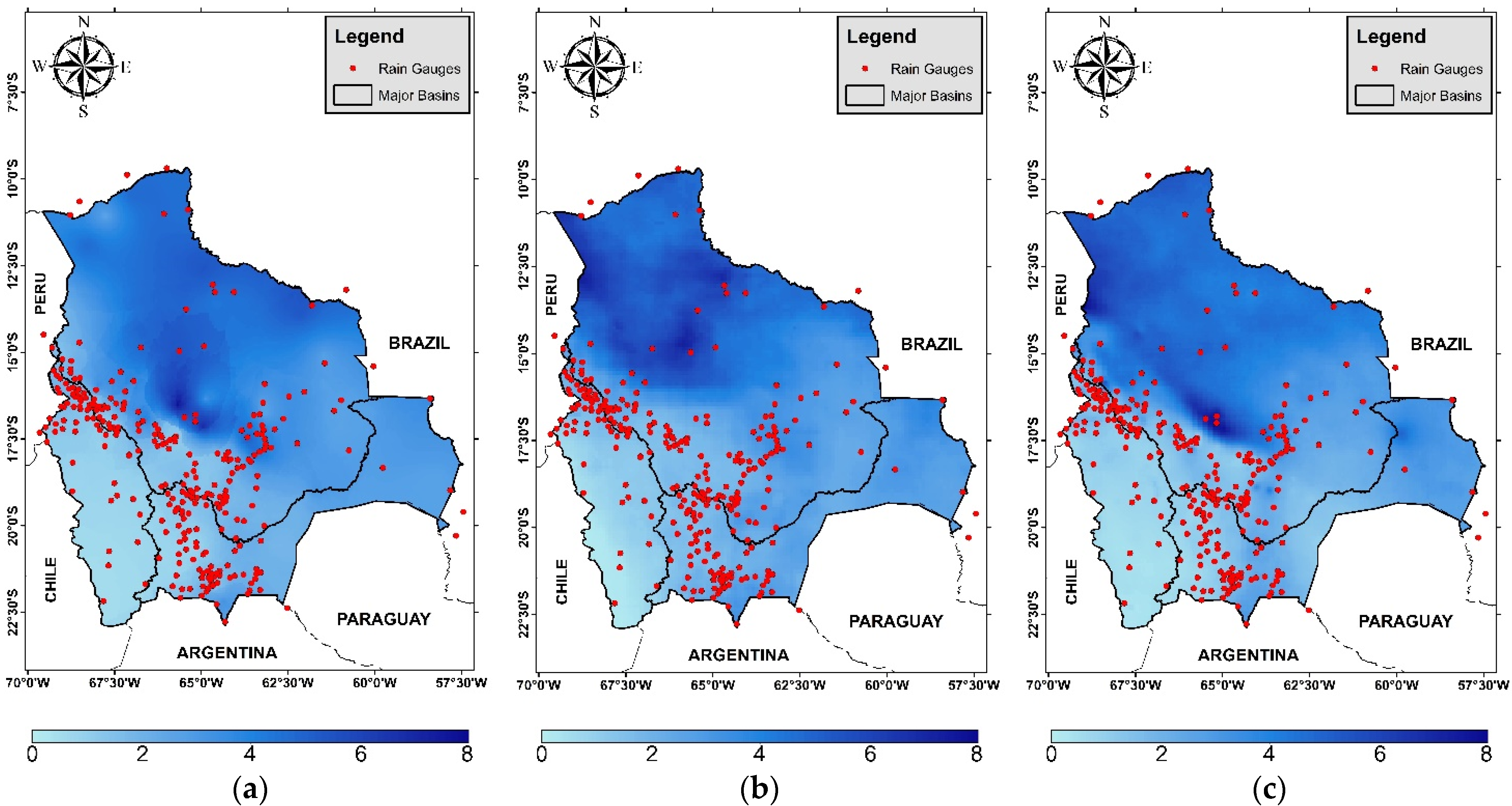
Figure 8.
Daily scatter plots of the SBP products for the: (a) Altiplano, (b) Amazon and (c) La Plata basins.
Figure 8.
Daily scatter plots of the SBP products for the: (a) Altiplano, (b) Amazon and (c) La Plata basins.

Figure 9.
Daily correlation coefficient map: (a) GSMaP and (b) CHIRPS.

Figure 10.
Average daily precipitation maps for the period 2001–2015 of: (a) rain gauges, (b) GS, (c) CH and (d) GMET.
Figure 10.
Average daily precipitation maps for the period 2001–2015 of: (a) rain gauges, (b) GS, (c) CH and (d) GMET.

Figure 11.
Daily scatter plots of the generated precipitation products for the: (a) Altiplano, (b) Amazon and (c) La Plata basins.
Figure 11.
Daily scatter plots of the generated precipitation products for the: (a) Altiplano, (b) Amazon and (c) La Plata basins.

Figure 12.
Daily correlation coefficient map: (a) GS, (b) CH and (c) GMET.
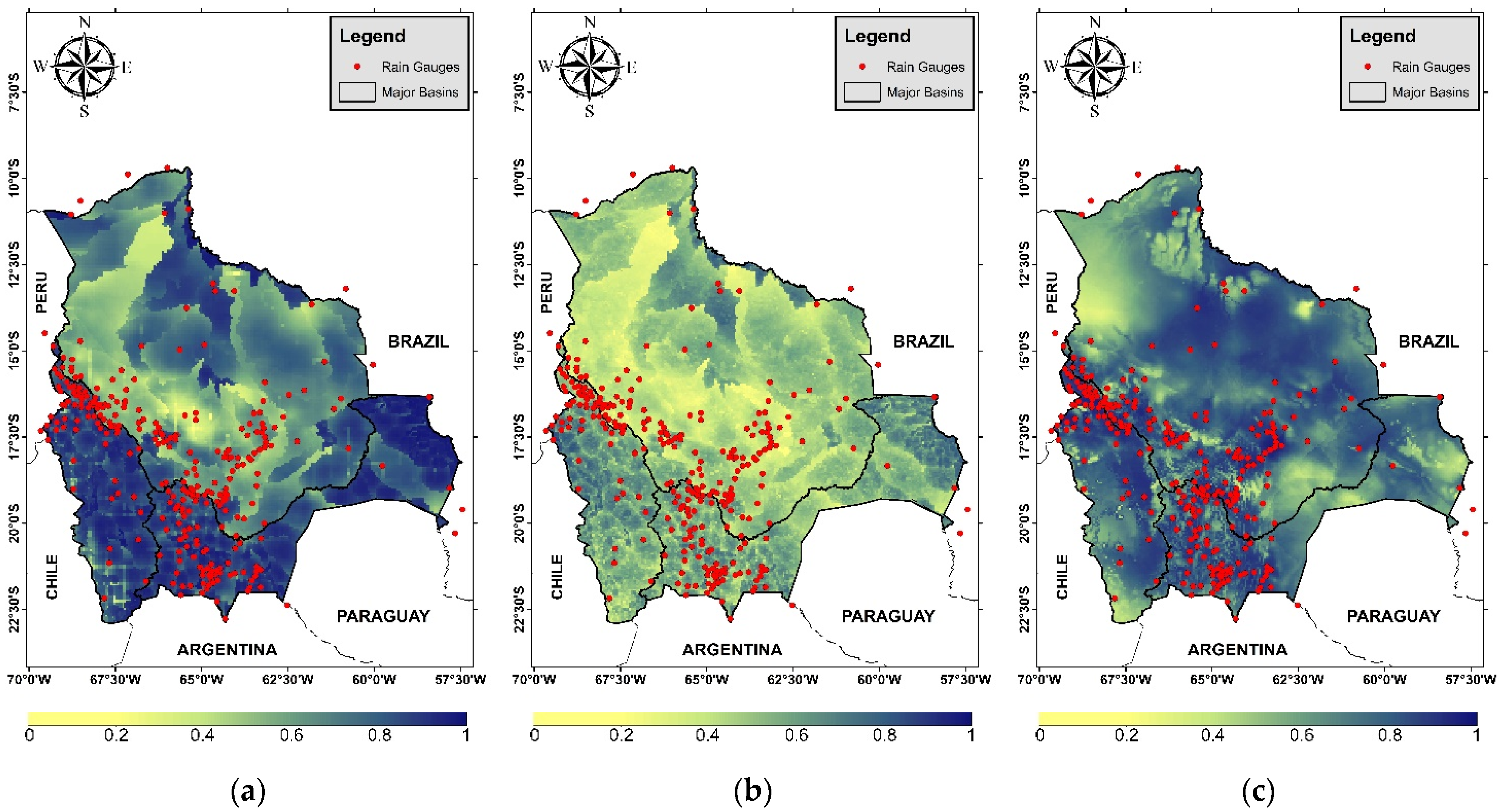
Figure 13.
(a) Rocha basin elevation map point and (b) average daily precipitation map for the period 2000–2015, with the Puente Cajón flow measuring station shown as a green triangle.
Figure 13.
(a) Rocha basin elevation map point and (b) average daily precipitation map for the period 2000–2015, with the Puente Cajón flow measuring station shown as a green triangle.

Figure 14.
(a) Rocha sub-basin map, (b) rain gauge accumulated precipitation, (c) GSMaP accumulated precipitation, (d) CHIRPS accumulated precipitation, (e) GS accumulated precipitation and (f) CH accumulated precipitation from 17 to 31 January 2014.
Figure 14.
(a) Rocha sub-basin map, (b) rain gauge accumulated precipitation, (c) GSMaP accumulated precipitation, (d) CHIRPS accumulated precipitation, (e) GS accumulated precipitation and (f) CH accumulated precipitation from 17 to 31 January 2014.

Figure 15.
Precipitation time series of simulated and observed river discharge at Puente Cajon Station, using various products: (a) rain gauge, (b) GSMaP, (c) CHIRPS, (d) GS and (e) CH.
Figure 15.
Precipitation time series of simulated and observed river discharge at Puente Cajon Station, using various products: (a) rain gauge, (b) GSMaP, (c) CHIRPS, (d) GS and (e) CH.


Table 1.
Statistics indicators for SBP products in relation to rain gauges.
| Altiplano Basin | Amazon Basin | La Plata Basin | Bolivia | |||||
|---|---|---|---|---|---|---|---|---|
| GSMaP | CHIRPS | GSMaP | CHIRPS | GSMaP | CHIRPS | GSMaP | CHIRPS | |
| Determination Coefficient (R2) | 0.35 | 0.38 | 0.37 | 0.28 | 0.33 | 0.25 | 0.36 | 0.29 |
| Correlation Coefficient (R) | 0.58 | 0.61 | 0.60 | 0.52 | 0.58 | 0.50 | 0.59 | 0.53 |
| Accumulated Bias (mm) | 3933.9 | 3115.3 | 11,450.8 | 12,363.9 | 8181.3 | 8581.7 | 8573.2 | 9030.3 |
| Relative Bias (%) | 9.14 | −7.91 | 5.56 | 1.55 | 12.49 | −3.92 | 6.78 | 0.29 |
| Mean Absolute Error (MAE) | 0.65 | 0.52 | 1.90 | 2.05 | 1.36 | 1.42 | 1.42 | 1.50 |
| Root Mean Square Error (RMSE) | 1.05 | 1.01 | 2.79 | 3.34 | 2.11 | 2.57 | 2.04 | 2.42 |
| Nash and Sutcliffe Efficiency (NSE) | 0.69 | 0.72 | 0.76 | 0.66 | 0.71 | 0.57 | 0.80 | 0.72 |
Table 2.
Statistics indicators for SBP-generated precipitation products in relation to rain gauges.
| Altiplano Basin | Amazon Basin | La Plata Basin | Bolivia | |||||||||
|---|---|---|---|---|---|---|---|---|---|---|---|---|
| GS | CH | GMET | GS | CH | GMET | GS | CH | GMET | GS | CH | GMET | |
| Determination Coefficient (R2) | 0.93 | 0.86 | 0.73 | 0.75 | 0.70 | 0.75 | 0.93 | 0.80 | 0.68 | 0.81 | 0.74 | 0.73 |
| Correlation Coefficient (R) | 0.97 | 0.93 | 0.85 | 0.86 | 0.83 | 0.86 | 0.96 | 0.89 | 0.81 | 0.90 | 0.86 | 0.85 |
| Accumulated Bias (mm) | 976.9 | 1336.7 | 1191.4 | 7478.5 | 7960.3 | 4810.9 | 2034.4 | 4035.0 | 4017.1 | 8573.2 | 6178.2 | 3390.2 |
| Relative Bias (%) | −12.03 | −22.86 | −10.00 | −32.90 | −34.96 | 4.04 | −13.75 | −29.78 | −2.25 | −29.04 | −33.64 | 2.46 |
| Mean Absolute Error (MAE) | 0.16 | 0.22 | 0.20 | 1.24 | 1.32 | 0.80 | 0.34 | 0.67 | 0.67 | 0.89 | 1.02 | 0.56 |
| Root Mean Square Error (RMSE) | 0.28 | 0.42 | 0.43 | 2.03 | 2.16 | 1.31 | 0.66 | 1.21 | 1.30 | 1.43 | 1.60 | 0.91 |
| Nash and Sutcliffe Efficiency (NSE) | 0.98 | 0.95 | 0.95 | 0.87 | 0.86 | 0.95 | 0.97 | 0.90 | 0.89 | 0.90 | 0.88 | 0.96 |
Table 3.
Statistical indicators of simulated river discharge at Puente Cajón Station.
| Rain Gauge | GSMaP | CHIRPS | GS | CH | |
|---|---|---|---|---|---|
| Determination Coefficient (R2) | 0.52 | 0.82 | 0.09 | 0.42 | 0.36 |
| Correlation Coefficient (R) | 0.72 | 0.91 | 0.30 | 0.65 | 0.60 |
| Mean Absolute Error (MAE) | 5.45 | 1.19 | 6.55 | 4.25 | 3.14 |
| Root Mean Square Error (RMSE) | 9.88 | 2.79 | 12.44 | 8.55 | 6.23 |
| Nash and Sutcliffe Efficiency (NSE) | −1.32 | 0.82 | −2.67 | −0.74 | 0.08 |
Publisher’s Note: MDPI stays neutral with regard to jurisdictional claims in published maps and institutional affiliations. |
© 2022 by the authors. Licensee MDPI, Basel, Switzerland. This article is an open access article distributed under the terms and conditions of the Creative Commons Attribution (CC BY) license (https://creativecommons.org/licenses/by/4.0/).
Share and Cite
MDPI and ACS Style
Saavedra, O.; Ureña, J. Generation of Combined Daily Satellite-Based Precipitation Products over Bolivia. Remote Sens. 2022, 14, 4195. https://doi.org/10.3390/rs14174195
AMA Style
Saavedra O, Ureña J. Generation of Combined Daily Satellite-Based Precipitation Products over Bolivia. Remote Sensing. 2022; 14(17):4195. https://doi.org/10.3390/rs14174195
Chicago/Turabian StyleSaavedra, Oliver, and Jhonatan Ureña. 2022. "Generation of Combined Daily Satellite-Based Precipitation Products over Bolivia" Remote Sensing 14, no. 17: 4195. https://doi.org/10.3390/rs14174195
Note that from the first issue of 2016, this journal uses article numbers instead of page numbers. See further details here.