Abstract
Global climate change profoundly influences the patterns of vegetation growth. However, the disparities in vegetation responses induced by regional climate characteristics are generally weakened in large-scale studies. Meanwhile, distinct climatic drivers of vegetation growth result in the different reactions of different vegetation types to climate variability. Hence, it is an extraordinary challenge to detect and attribute vegetation growth changes. In this study, the spatiotemporal distribution and dynamic characteristics of climate change effects on vegetation growth from 2000 to 2020 were investigated by the normalized difference vegetation index (NDVI) dataset during the growing season (April–October). Meanwhile, we further detected the climate-dominated factor between different vegetation types (i.e., forest, shrub, and grass) within the Chaohe watershed located in temperate northern China. The results revealed a continuous greening trend over the entire study period, despite slowing down since 2007 (p < 0.05). Growing-season precipitation (P) was identified as the dominant climatic factor of the greening trend (p < 0.05), and approximately 34.83% of the vegetated area exhibited a significant response to increasing P. However, continued warming-induced intensive evaporation demand caused the vegetation growth to slow down. Hereinto, the areas with a significantly positive response of forest growth to temperature decreased from 24.38% to 18.06% (p < 0.05). In addition, solar radiation (SW) corresponds to the vegetation trend in the watershed (p < 0.05), and the significantly positive SW-influenced areas increased from 9.24% and 2.64% to 11.78% and 3.37% in forests and shrubland, respectively (p < 0.05). Our findings highlight the nonlinearity of long-term vegetation growth trends with climate variation and the cause of this divergence, which provide vital insights into forecasting vegetation responses to future climate change.
1. Introduction
Vegetation and climate system interactions are governed by complex biophysical factors and processes, which pose significant challenges for natural resources managers. For instance, terrestrial vegetation growth affects global carbon–water cycles, such as reducing atmospheric CO2 concentration via photosynthesis and regulating water flux through transpiration in the soil–vegetation–atmosphere continuum [1]. In turn, climate variabilities also induce rapid alterations in vegetation growth and regional carbon–water coupling processes [2], which influence vegetation adaptation and ecosystem resilience [3,4]. Therefore, revealing the role of climate change in driving vegetation growth is particularly significant in coping with and predicting potential climatic threats [5].
Vegetation has experienced a greening trend throughout the majority of vegetated surfaces since the 1980s [6]. However, regional differences in climate characteristics trigger the disparities in vegetation responses that are generally weakened at a large scale [7,8]. For example, rising temperatures promote vegetation growth above 30°N [9]. However, frequent droughts and nonlinear responses of photosynthesis to these temperatures has limited vegetation growth in north temperate and arctic ecosystems [9,10,11]. In addition, the global greening trend highlighted the heterogeneity of dominant climatic factors for regional vegetation dynamics [12,13]. Previous studies found that ample precipitation contributed to vegetation growth in water-stress regions, such as South Africa [14]. However, excessive precipitation in extreme wet years also slowed down the vegetation growth in central U.S.A [15]. Meanwhile, as one of the vital elements in vegetation growth, increased vapor pressure deficit (VPD) potentially hastens atmospheric drought-induced mortality via carbon starvation or hydraulic failure [16,17]. Therefore, associated with increasing temperature, VPD influences vegetation growth and regional hydrological processes [18]. Moreover, as the critical energy source for vegetation growth, solar radiation variations also affect vegetation greening trends. Recent studies revealed that solar dimming explained 80% of the decline in crop growth across North China [19]. Therefore, given the complex response of vegetation to climate variations, how vegetation reacts to distinct regional climatic characteristics is still a pendent issue [20,21].
Due to different climatic and other environmental adaptabilities of vegetation growth [22], studies found the responses of different vegetation types to climate variability were distinct [22,23,24,25]. To explain, more than 60% of the forests’ and shrubs’ dynamics across China could be explained by precipitation variability [26,27]. However, studies also revealed a higher correlation between meadow dynamics and temperature than water supply [28]. This divergence of results is due to the distinct climate sensitivity of different vegetation responses more researches are needed for specific vegetation types and localities. Therefore, the primary objectives of our study were: (1) to reveal the spatio-temporal distribution and dynamic characteristics of climate change effects on vegetation growth during the growing season (April–October) from 2000 to 2020; (2) to detect the dominate climate -factor between different vegetation types (i.e., forest, shrub, and grass) within the Chaohe watershed (hereafter referred to as the CHW) located in temperate northern China. To this end, we firstly diagnosed spatio-temporal evolution and abrupt changes in vegetation trends based on NDVI data of the watershed, which is the prerequisite for revealing vegetation growth driving mechanisms. Secondly, we analyzed the responses between vegetation growth and climatic factors and revealed the determinant. Further, we gridded climate data for the forests, shrubs, and grasses to identify the dominant climate factors for different vegetation type over the CHW, which is the primary reservoir watershed for Beijing’s drinking water supply.
2. Methods
2.1. The Chaohe Watershed
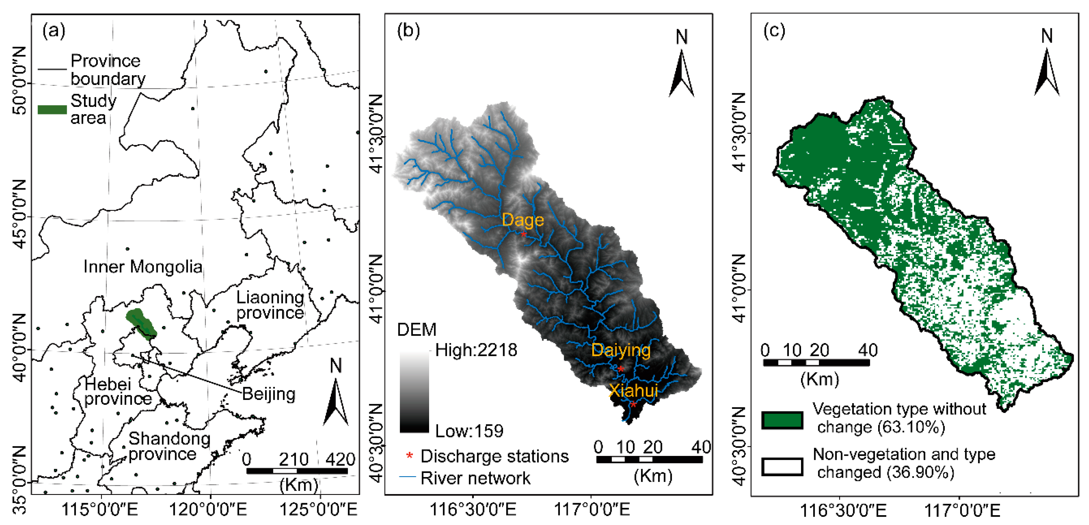
The domain for our study (the Chaohe watershed) is the essential water source region of Miyun Reservoir, and it provides more than 70% of the drinking water for the urban population in Beijing [22]. This domain is located in northern China (116°08′–117°28′E, 40°34′–41°37′N, Figure 1a) with an elevation between 159–2218 m above the sea level and a drainage area of approximately 4.85 × 10³ km2 (Figure 1b).
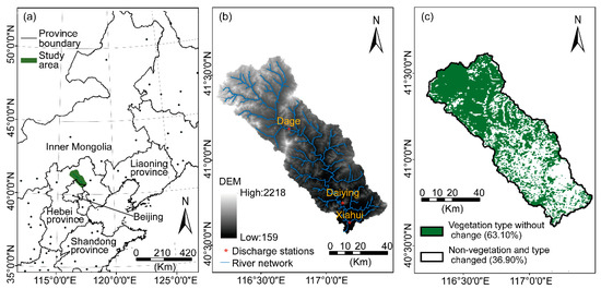
Figure 1.
Geographic information of the study area: location of the Chaohe watershed and adjacent provinces in China (a), digital elevation model (DEM) map and (b), areas of vegetation types without changing during 2000–2019 (c).
The mean annual temperature (MAT) and precipitation (MAP) are 12.50°C and 503.01 mm (2000–2020), respectively. The East Asian summer monsoon transfers moisture over the watershed, which accounts for above 80% of the annual precipitation.
The land cover is dominated by shrubland, forestland (evergreen needleleaf forests, deciduous broadleaf forests, mixed forests), and grassland, which accounts for above 80% of the watershed [29,30]. In addition, cropland, residential areas, and bare areas account for a small percentage of the watershed [31]. Prior to this study, we ascertained the area without vegetation types changing, according to the watershed’s land-use change during the entire study period (Figure 1c).
2.2. Data and Sources
2.2.1. Meteorological and Satellite-Based Data
The monthly gridded meteorological data over the study period from 2000 to 2020, including temperature (Ta), precipitation (P), vapor pressure deficit (VPD), wind speed (Vs), and solar radiation (SW), were downloaded from the TerraClimate product (Table 1), with 2.5 arc minutes of high spatial resolution [26].

Table 1.
The climate factors used in this study.
TerraClimate product was interpolated by thin-plate splines in the Climatic Research Unit (CRU) Time series version 4.0 based on station observations [32], and was validated against the Global Historical Climatology Network (GHCN) database [32,33]. Meanwhile, the TerraClimate dataset is also widely used in many studies [13,34,35].
Land cover information with 500 m of spatial resolution for the years 2000 and 2019 was derived from the Moderate Resolution Imaging Spectroradiometer (MODIS) Land Cover Type Version 6 (MCD12Q1) product [36]. All types of land cover over the watershed provided by the product include evergreen needleleaf forests, deciduous broadleaf forests, mixed forests, shrublands, grasslands, croplands, water bodies, urban land, and barren land [37]. Additionally, we reclassified them using the Geographic Information System for forestland (merging evergreen needleleaf forests, deciduous broadleaf forests, mixed forests), shrubland, grassland, croplands, water bodies, urban area, and barren land (Figure S1). Meanwhile, we compared each land cover type between the year 2000 and the year 2019 to clarify the area without change and used it for further analysis (Figure 1c). In this study, the vegetation coverage mentioned mainly included forestland, shrubland, and grassland.
2.2.2. Satellite-Derived Vegetation Index Datasets
NDVI datasets are frequently used for monitoring terrestrial vegetation growth at regional and global scales [38]. In this study, we analyzed the characteristics of vegetation growth, covering the study period from 2000 to 2020, as the product of MODIS 16-day NDVI (500 m spatial resolution), which was extracted from the MOD13A1 Version 6 Vegetation Index Product [39]. The product was validated in strong agreement across a global set of biome types and applied successfully in many studies [40,41,42,43]. Firstly, pixels with an average NDVI above 0.1 from April to October were extracted for the analyses. Then, we applied the nearest neighbor interpolation method to match the raw climate datasets to the NDVI data during the study period. Meanwhile, time series of the watershed annual average NDVI from 2000 to 2020 were calculated via an area-weighted average of all the pixels with NDVI.
In this study, satellite-derived meteorological and vegetation index datasets were extracted from the Google Earth Engine (GEE), which provided online access to archived satellite image data. We analyzed and downloaded the satellite-based NDVI and meteorological data in the GEE environment via the programming code editor (namely GEE Code Editor) using Python (https://code.earthengine.google.com/, accessed on 6 April 2021).
The inter-annual meteorological and NDVI trajectory method was used to detect the spatial distribution of climate variation and vegetation growth. After that, we superimposed the results of the NDVI trend onto land use information to identify the dynamic of each vegetation type. The raw NDVI data were detrended before analysis of the variability [7].
2.3. Change Characteristics Detection and Climatic Factors Analysis
Based on growing season NDVI and meteorological data series from 2000 to 2020, we first diagnosed whether and when NDVI changed abruptly in the watershed using the Breaks for Additive Seasonal and Trend (BFAST) algorithm [44]. This algorithm decomposes the NDVI time series into seasonal, trend, and residual components [38]. The BFAST package version 1.6.1 in R Studio version 1.4.1106 was applied to decompose the meteorological and NDVI time series in this study [45]. This algorithm iteratively fits the trend component by the piecewise linear model to the sections of the NDVI time series and detects whether abrupt changes occur [46,47]. Further, the number and timing of abrupt changes were determined via the Bayesian information criterion and by minimizing the residual sum of squares, respectively [30,31,34]. Consequently, we had 294 observations of 16-day NDVI data for over 21 years of the growing season for the analysis. The general form of this model is as follows:
where Yt is the observed data at time, t; Tt is the trend component, St is the seasonal component, and et is the remainder component [48]. We divided the entire study period into before and after the abrupt change period, and further identified vegetation and climate factors’ spatiotemporal patterns and trends. Hereinto, the linear regression analysis was used to analyze the trends of the NDVI and climate factors on a pixel scale, respectively. Due to the different order of magnitudes in the trend of NDVI and climate factors, we unified all the units presented (per decade) in full text. The slope in the fitting regression equation was calculated by the ordinary least squares method, namely the inter-annual change [49]. Additionally, while a positive slope typically indicates (NDVI increased) vegetation greening, it instead indicated vegetation browning (NDVI decreased). This analysis and process were operated in MATLAB R2018a.
Meanwhile, the Hurst exponent (He) was widely applied in climatology and vegetation studies to assess the durability of changes in time series data over long periods [22,50,51]. Thus, we used the He to evaluate the persistence of the NDVI time series (Figure 2). The MATLAB R2018a function was applied to compute the Hurst exponent according to the following procedure.
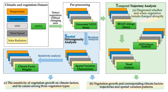
Figure 2.
Flow chart of this study. The green arrow and panel represent the time-varying analysis, and the blue arrow and panel represent spatial analysis.
Firstly, define the NDVI time series [NDVI(t)] (t = 1, …, n). Additionally, calculate the average sequence of the NDVI time series,
Secondly, calculate the accumulated deviation and create the range sequence,
Thirdly, obtain the standard deviation (SD) sequence and further calculate the Hurst exponent (He),
The He value was calculated by fitting a simple linear regression in Equation (7), which is the slope of the resulting equation,
where n is the number of years during 2000–2020; c is a constant.
The He (expanded from 0 to 1) equals 0.5, indicating the future NDVI is a stochastic series. When the He is less than 0.5, it forecasts that the future NDVI series will exhibit the opposite tendency to the current trend. Conversely, when the He is greater than 0.5, it suggests a similar trend in the future NDVI [52].
Residual analysis was applied to differentiate the influence of climate factors and anthropogenic disturbances on NDVI changes [53]. Based on the MATLAB R2018a, the predicted NDVI (NDVIpred) in each pixel was computed by the multiple correlation regression (MCR) which built the prime relationship with selected climatic factors [54], as follows:
where atem, apre, avpd, avs, asw, and a0 are the regression coefficients determined by the least square method; Mtem, Mpre, Mvpd, Mvs, and Msw are the climatic factors that impact the NDVI.
According to Equation (9), NDVI residuals (NDVIres) and differences between the observed (NDVIobs) and predicted NDVI were detected. Then, the potential impacts of anthropogenic disturbances on growing season NDVI changes were isolated using the residual trend analysis: if the residuals trend is insignificant (p-value exceeds 0.05), it indicates that the NDVI changes could be explained by selected climatic factors. Otherwise, a p-value below 0.05 indicates vegetation changes, also influenced by anthropogenic disturbances, are not fully explained by climate factors [7].
Finally, we determined climatic determinants for vegetation growth, as mentioned in previous studies, based on the loadings of the stepwise multiple linear regression [55]. The collinearity was diagnosed before analysis using the variance inflation factor (VIF). The climate factors were retained with a VIF of less than 10 [12,37].
3. Results
3.1. Spatiotemporal Changes in Vegetation Growth and Climate Factors
3.1.1. NDVI Trajectory and Spatial Variations
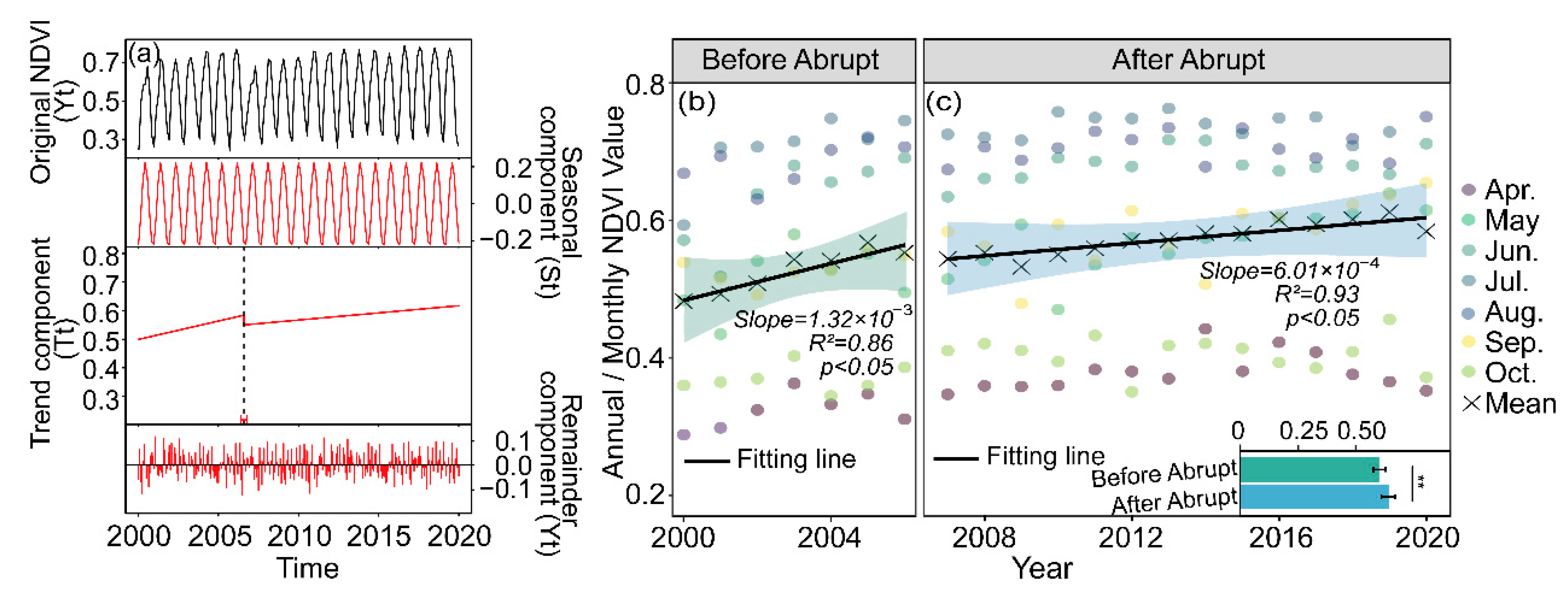
For the entire period of 2000–2020, the inter-annual variation of the April to October growing season NDVI over the watershed indicated a significant greening trend, with a breakpoint identified in 2007 (Figure 3a, p < 0.05). Based on the breakpoint, we divided the entire study period into before and after the abrupt change periods, respectively. Meanwhile, we further analyzed the linear trends in NDVI during the two periods and found that the NDVI trend slowed down to 6.01 × 10⁻³ per decade after 2007 (Figure 3c, p < 0.05), which was nearly half of that before (1.32 × 10⁻² per decade, Figure 3b, p < 0.05).
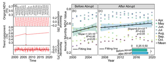
Figure 3.
BFAST detected as a breakpoint (black dotted line). Yt is the raw NDVI data, St is the fitted seasonal cycle, Tt is the trend component and et is the BFAST residuals (a), the NDVI changes during the growing season (April to October) over the period from 2000 to 2020 within the Chaohe watershed: annual mean and monthly NDVI before (b) and after (c) the abrupt change in 2007 over the CHW. Asterisks (**) denote significant differences between the NDVI value before and after the abrupt change (p < 0.01).
We calculated the annual average growing season NDVI (NDVIave) during the study period from 2000 to 2020, and the spatial distribution of the NDVIave is depicted in Figure 4a. In the CHW, NDVIave increased gradually from the upstream to the southeast, with higher NDVI values (peaked at 0.85) appearing over the forests in southern regions, while the lower values (lowest value is 0.18) occurred in regions near the river network.
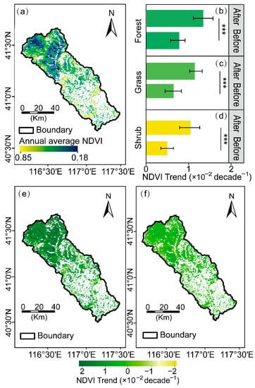
Figure 4.
NDVI changes during the growing season (April to October) from 2000 to 2020 within the Chaohe watershed. Spatial distributions of annual average NDVI at the growth season scales during 2000–2020 (a), averaged annual NDVI changes before and after the abrupt change by three vegetation types: forest (b), grass (c), and shrub (d), respectively; Spatial distribution of NDVI trend before (e) and after (f) abrupt change. Asterisks (***) denote significant differences between the NDVI trend before and after the abrupt change (p < 0.001).
In addition, there were distinct NDVI temporal and spatial characteristics for three vegetation types. Specifically, the moderating upward trend was exhibited among three vegetation types after an abrupt change in 2007 (Figure 4b–d). Hereinto, the greening trend in forests was higher than that in grasses and shrubs with the slope of 1.38 × 10⁻² per decade before the abrupt change (p < 0.05, Figure 4b), which slowed down to 7.52 × 10⁻³ per decade. Additionally, the variation trend in grasses and shrubs declined from a rate of 1.21 × 10⁻² and 1.07 × 10⁻² per decade to 6.02 × 10⁻³ and 4.89 × 10⁻³ per decade, respectively (p < 0.05, Figure 4c,d).
Spatially, around 39.38% of the vegetated area presented a significant greening trend (p < 0.05, Figure 4e). Hereinto, 54.70% of forestland showed a significant trend in the overall forestlands (p < 0.05). The areas with a significant greening trend in grassland and shrubland were 48.37% and 47.28% of the overall grassland and shrubland, respectively (p < 0.05). Meanwhile, the browning trend (i.e., the negative slope of the NDVI trend) areas were interspersed in the central area of the watershed, which occupied approximately 1.42% of the total vegetated area before the abrupt change.
However, the significantly increased NDVI areas declined to 31.54% of the total vegetated area after 2007 (p < 0.05, Figure 4f). Hereinto, 42.14% of forestland presented a significant greening trend, followed by grassland (39.76% of the total grassland area), and shrubland (35.96% of the total shrubland area), respectively.
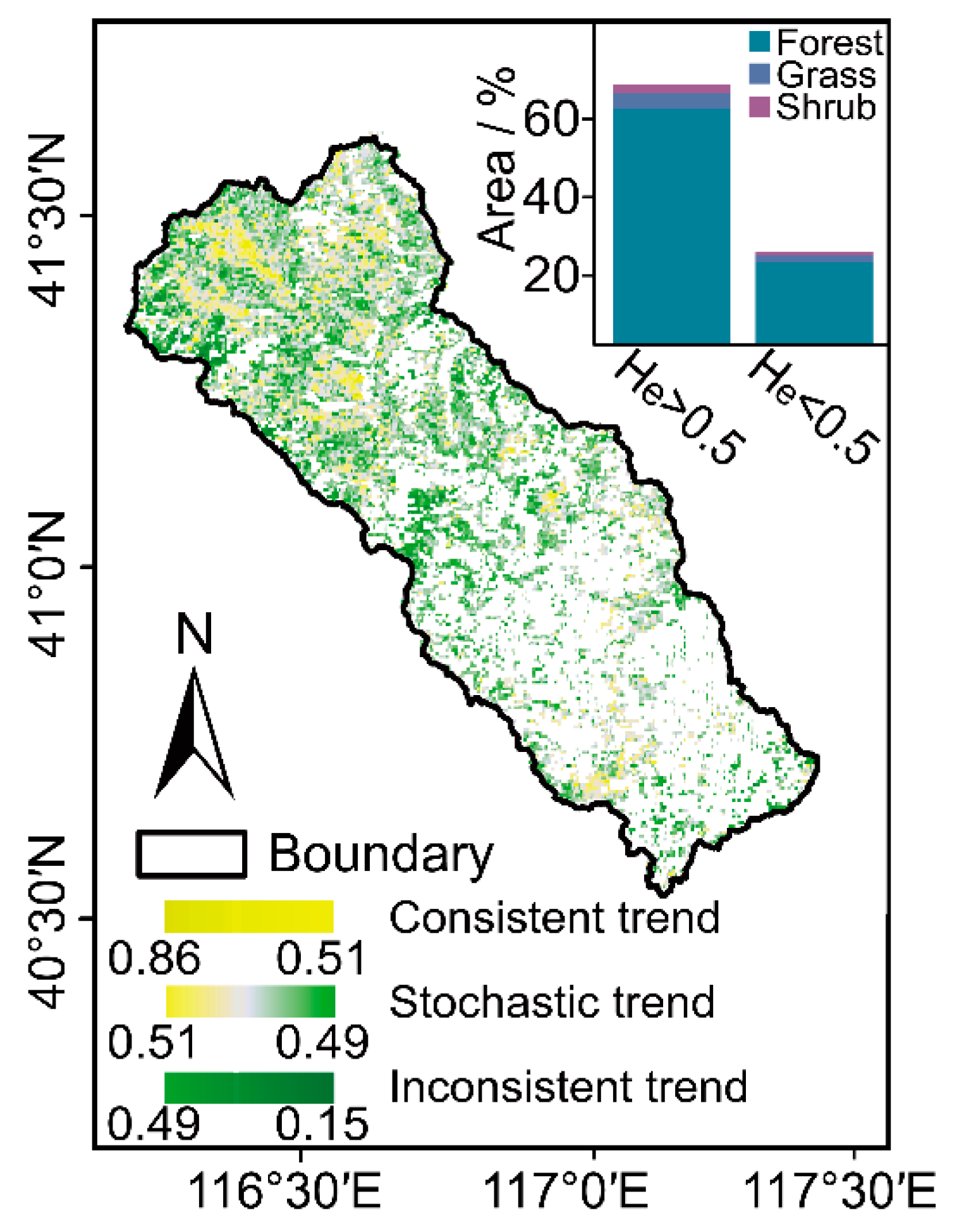
The consistency of future vegetation dynamic trends is shown in Figure 5. There was a distinct decrease in the He of the annual average NDVI time series from high altitude to low altitude in the CHW, with the spatial distribution of the He ranging from 0.15 to 0.86 (Figure 5). Hereinto, 64.97% of the total vegetated areas had He values exceeding 0.5, which indicates the consistent change trend of NDVI after the entire study period. The forestlands, grasslands, and shrublands account for 61.28%, 2.65%, and 1.04%, respectively. By contrast, 27.62% of the vegetated areas with He values below 0.5 portended the inconsistency of vegetation dynamic trends after the study period in the watershed. Hereinto, the forestlands account for 22.74% followed by the grasslands (3.07%) and shrublands (1.81%). For the rest of the areas mentioned above (i.e., He ≈ 0.5), primarily distributed near river networks and water bodies, the future NDVI change trend would exhibit stochastic fluctuation.

Figure 5.
Spatial distribution of He (the inset graph shows the area percentage of each vegetation type).
In addition, we superimposed the results of the NDVI trend with the He results to reveal the variation in trends and the consistency of the vegetation growth (Table 2). Overall, vegetation over the CHW will exhibit amelioration (positive NDVI trend) in the future. Hereinto, up to 59.54% of the vegetation area exhibited consistency and amelioration and is mainly distributed in forestlands, followed by grasslands and shrublands. Additionally, the inconsistency and amelioration accounted for 5.43%. Moreover, 25.50% of the vegetation area presented a consistent degradation trend (negative NDVI trend), mainly exhibited by forestlands, followed by grasslands and shrublands. In addition, a portion of 2.12% of the vegetation area will degrade in the future, although this trend is inconsistent.
Table 2.
The contrast between the NDVI change trend and the Hurst exponent (He).
3.1.2. Patterns of the Climatic Factors: Spatial vs. Temporal Characteristics
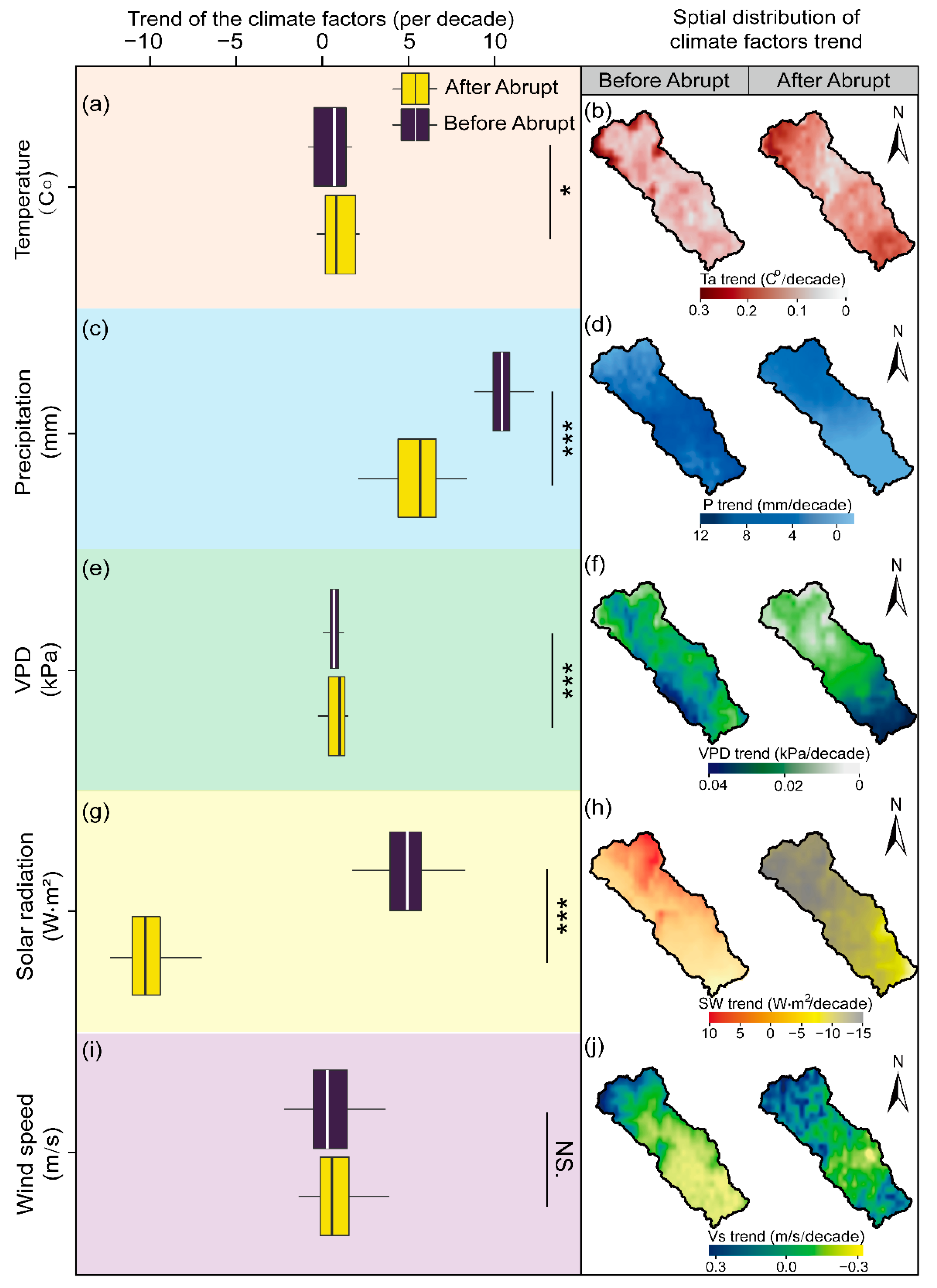
Spatial patterns of each climate factor (e.g., Ta, P, VPD, SW, and Vs) are depicted in Figure 6. Overall, the average growing season Ta was 20.94 °C within the 19.37 to 22.04 °C range during the study period. Significant warming patterns were presented across the entire study period with a rate of 0.24 °C per decade (Figure 6a, p < 0.05). The Ta uptrend was mainly exhibited in marginal areas in the northwest region and gradually weakened to the southeast before the abrupt change (the left column in Figure 6b). Nevertheless, the distinct Ta change trend had occurred since 2007, with a higher value in the northwest and southeast of the watershed, and a gradual decline to the center area (the right column in Figure 6b).

Figure 6.
Temporal-spatial changes of climate factors during April and October from 2000 to 2020 in the Chaohe watershed. Temporal changes of Ta (a), P (c), VPD (e), SW (g), and Vs (i). Spatial changes of Ta (b), P (d), VPD (f), SW (h), and Vs (j). Asterisks are significant at different levels: *** p < 0.001 and * p < 0.05. NS. indicates the insignificant differences between the climate factors trend before and after the abrupt change.
Meanwhile, the annual average P during the same study period was 441.95 mm within the 351.24 to 508.49 mm range. A significant upward trend was exhibited in annual P, at a rate of 10.82 mm per decade (Figure 6c, p < 0.05). Additionally, high values appeared in the center and in parts of the southeast regions (the left column in Figure 6d), before gradually declining at the northwest and the west of the downstream watershed. A weak increasing trend was found from 2007, with an average change rate of 6.67 mm per decade.
Furthermore, the annual average VPD ranged from 0.87 to 1.30 kPa (with an average value of 1.11 kPa). A significantly increased rate of 0.04 kPa per decade after the abrupt change (accounted for approximately 39.20% of the watershed, p < 0.05, Figure 6e), which mainly occurred in the south of the watershed (the right column in Figure 6f).
SW exhibited an inconsistent change trend before and after the abrupt change (Figure 6g). Specifically, SW significantly declined at a rate of 10.7 W m2 per decade in the northwestern regions of the watershed from 2007 to 2020 (the right column in Figure 6h, p < 0.05). However, an upward trend was detected from 2000 to 2007 (p < 0.05, the left column in Figure 6h).
The annual average wind speed was 2.29 m s–1 within the 2.13 to 2.61 m s–1 range. Due to there being no significant variations in Vs across the whole research period (Figure 6i,j, p = 0.56), no additional analysis for it is provided.
3.2. Response Patterns of the Vegetation Growth to Climatic Factors
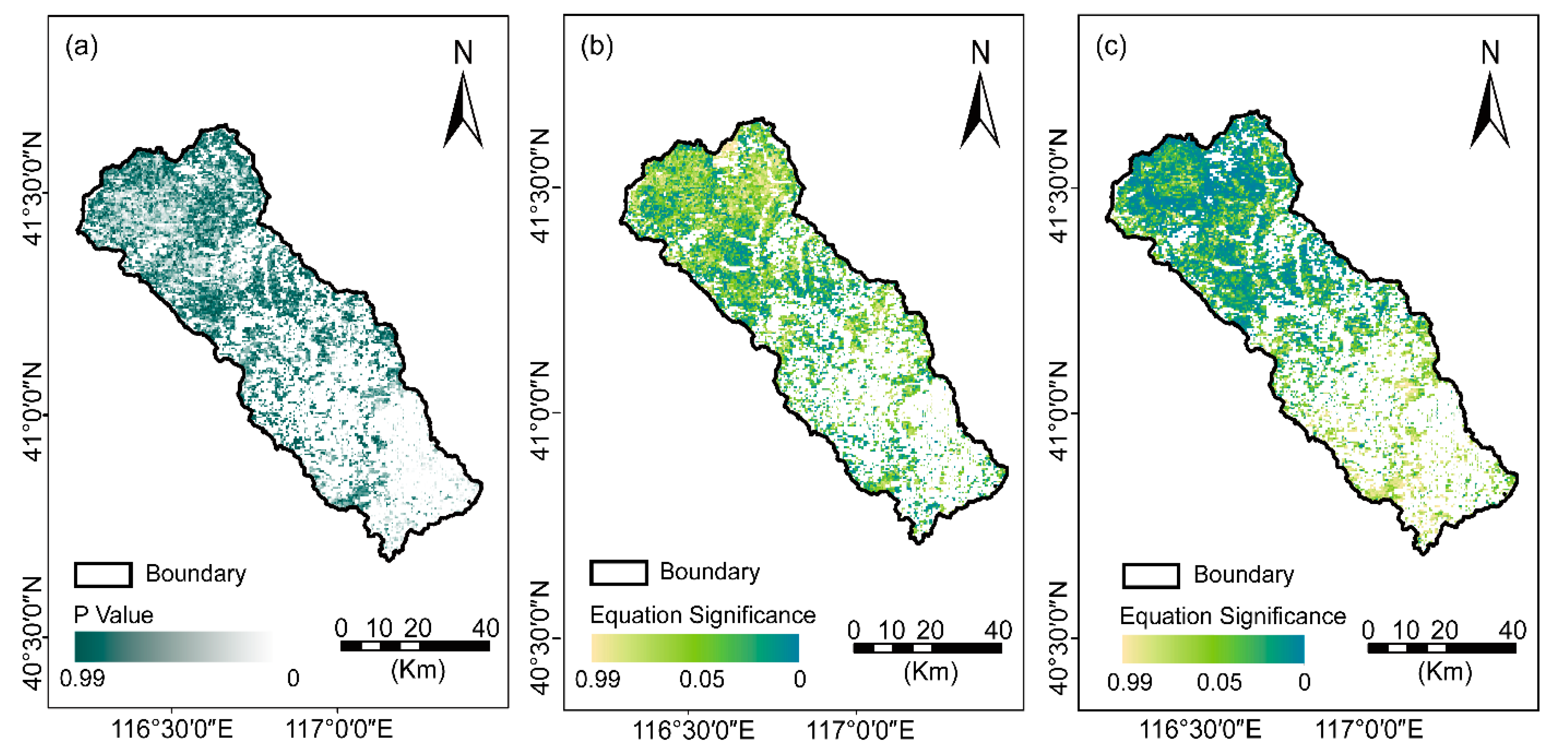
To isolate the potential anthropogenic disturbances to NDVI changes, the growing season NDVI residuals trend was analyzed by using MCR, with the selected climatic factors referring to Ta, P, VPD, and SW from 2000 to 2020. Further, the residual trend was analyzed and classified into significant and insignificant trends (Figure 7a). Approximately 95.50 percent of the vegetation areas exhibited an insignificant residual trend, which indicated NDVI changes could be explained by the selected climatic factors (the dark green and dark gray regions in Figure 7a). In addition, pixels of a light green and dark blue color showed significant trends (p < 0.05, Figure 7b,c), and indicated that vegetation changes in these areas were well explained by the MCR model fitted by Ta, P, VPD, and SW. Additionally, these areas might be slightly influenced by anthropogenic disturbances.
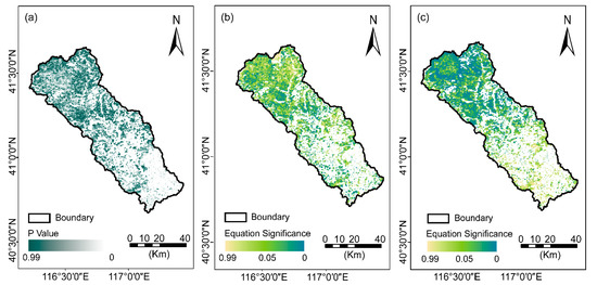
Figure 7.
The significance of the NDVI residuals (a), the spatial distributions of multiple regression equation significance before (b) and after the abrupt change (c) over the Chaohe watershed.
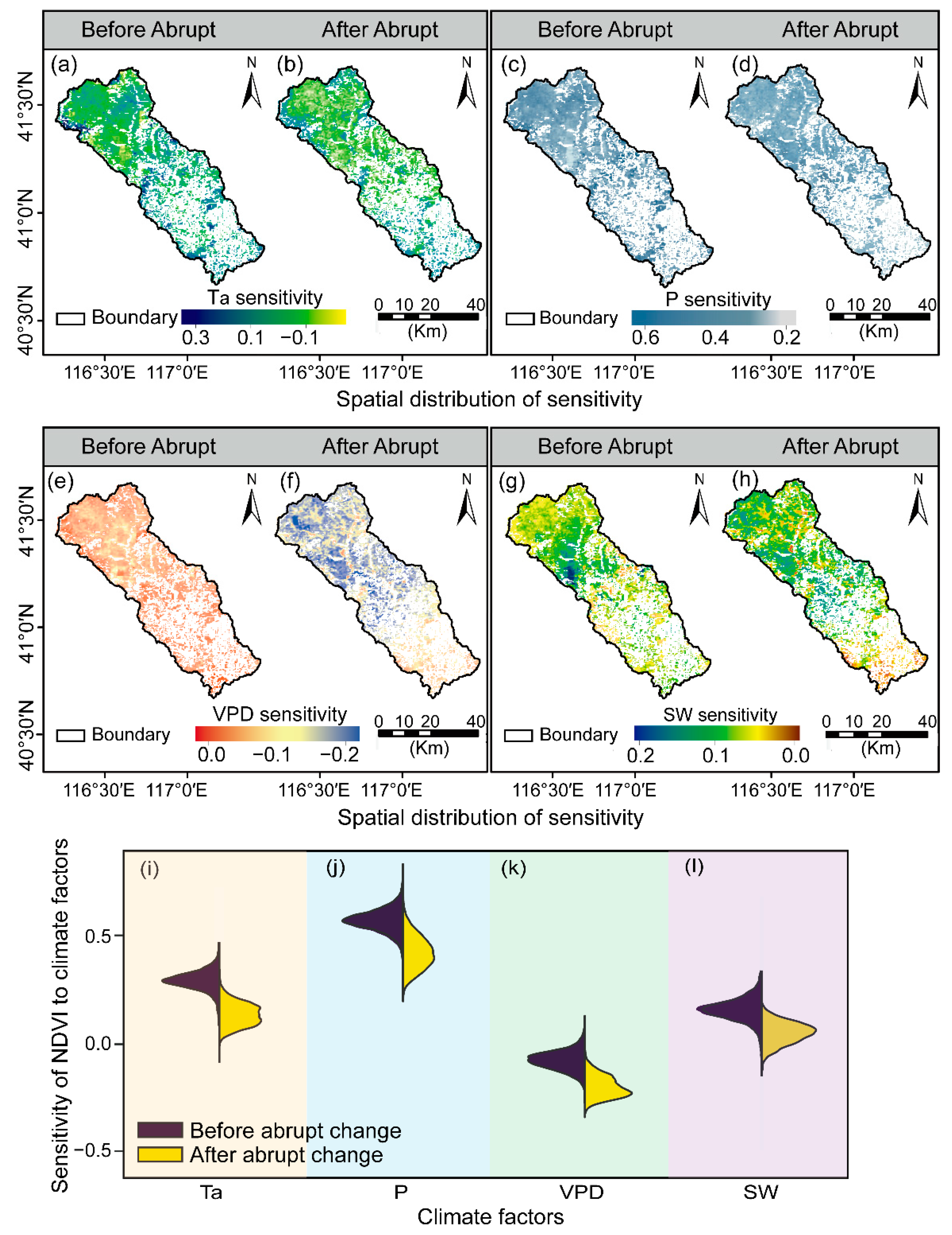
We explored the driving mechanisms of the NDVI spatiotemporal responses and found that P dominated vegetation growth throughout the watershed (Figure 8). Approximately 34.83% of the vegetated areas exhibited a significantly positive relationship between P and NDVI before the abrupt change, mostly in the central and northern regions (p < 0.05, Figure 8c). Additionally, a fraction of vegetated areas presented a negative response to P, primarily in the southeastern regions (not significant, Figure 8d).
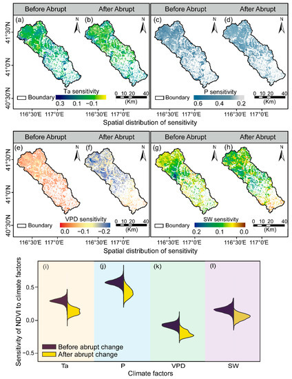
Figure 8.
Temporal-spatial variations in vegetation-climate sensitivity change during April and October from 2000 to 2020 within the Chaohe watershed. Spatial changes of Ta before (a) and after the abrupt change (b); P before (c) and after the abrupt change (d); VPD before (e) and after the abrupt change (f); SW before (g) and after the abrupt change (h); sensitivity’s temporal changes of Ta (i); P (j); VPD (k) and SW (l).
Ta also had a positive driving influence on vegetation growth (Figure 8a,b). A significantly positive influence of Ta on vegetation growth was exhibited in 25.94% of the total vegetated area before 2007, primarily in the northwest fringe parts and a portion in the central and lower areas. However, a small portion of the north area (i.e., around 4.07%) demonstrated a significantly negative response to Ta (Figure 8a). In addition, with continued climate warming, the beneficial influence of Ta weakened gradually over the northwest regions (Figure 8b,i), and the negative sensitivity of NDVI to Ta grew to 8.52% of the total vegetated area after the abrupt change (Figure 8b).
Generally, negative correlations of VPD with NDVI were exhibited (Figure 8e,f). Prior to 2007, 16.25% of the vegetated area reacted considerably, with the majority of the response occurring in the southeast, and a fraction in the marginal areas in the northwest (p < 0.05, Figure 8e,k). Additionally, with continuously increasing VPD, the vegetated area exhibited a significantly negative response to VPD, which increased to 19.27% between 2007 and 2020. (p < 0.05, Figure 8f,k).
To investigate the effect of solar radiation on vegetation growth, we also investigated partial correlations of NDVI with SW interannual fluctuations (Figure 8g,h,l). These correlations with radiation are generally weaker than those found for temperature and precipitation. Hereinto, increasing SW promoted the vegetation growth with the highest sensitivity region located in the western part of the upper reach. Vegetation growth reacted favorably to increased SW, with 13.25% of these areas exhibiting a substantial reaction before the abrupt change (p < 0.05, Figure 8g). Subsequently, the areas with a significantly positive correlation fell to 11.83% of the total vegetated area, primarily in the southern regions (p < 0.05, Figure 8h,l).
3.3. Climate Sensitivity between Different Vegetation Types
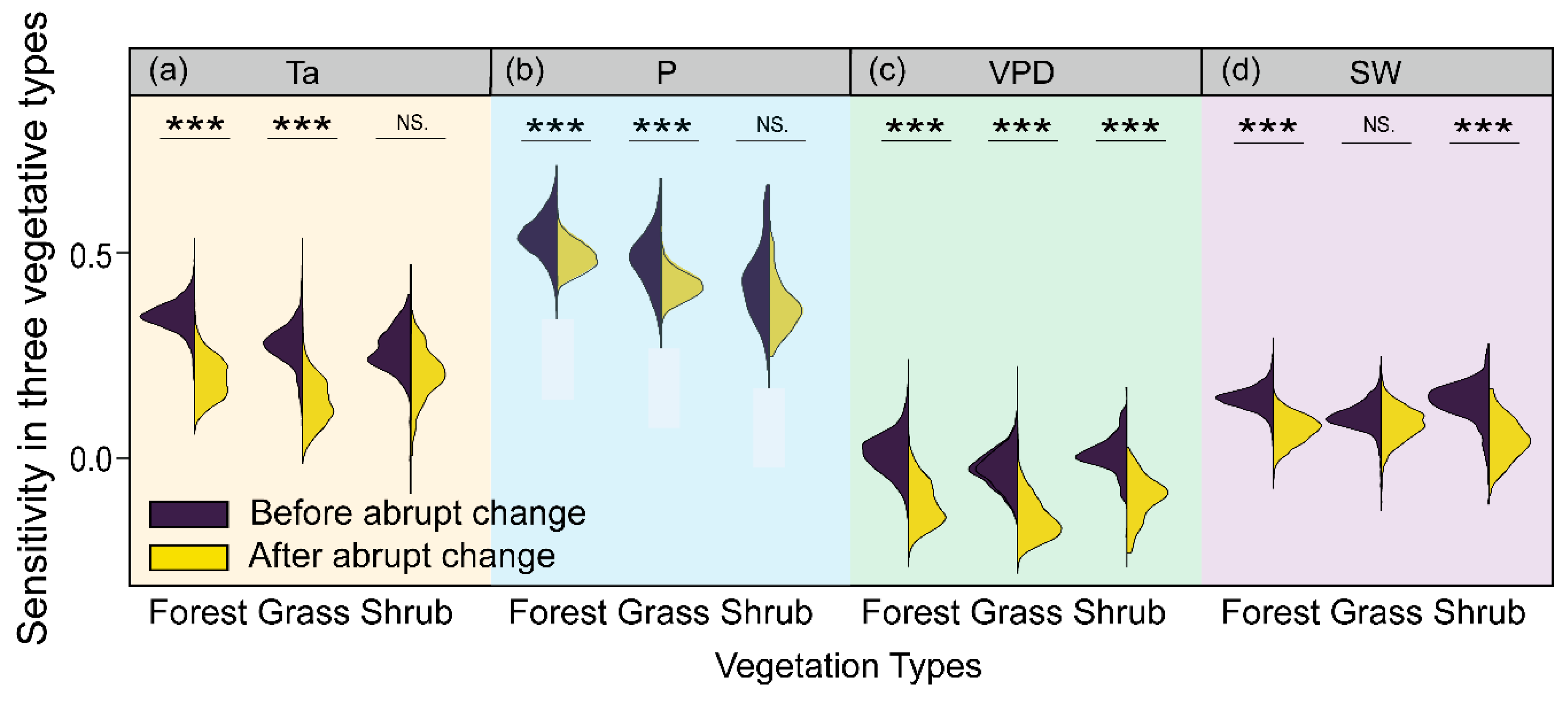
Distinct vegetation responses to climate factors among different vegetation types are depicted in Figure 9. Specifically, significant differences were observed in the response of forests and grasses to Ta and P before and after the abrupt change (p < 0.001, Figure 9a,b). The areas with a positive Ta influence decreased from 2007 to 2020, compared with the first period. Significant responses of plant growth to warming accounted for 24.38% of forests initially, and then fell to 18.06% as Ta continued to climb.
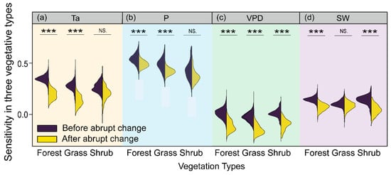
Figure 9.
Sensitivity’s temporal changes among three vegetation types: Ta (a), P (b), VPD (c), and SW (d). Asterisks (***) denote significant differences between the sensitivity before and after the abrupt change (p < 0.001). NS. indicates the insignificant differences between the sensitivity before and after the abrupt change.
Additionally, three vegetation types exhibited significant differences in VPD sensitivity before and after the abrupt change (p < 0.001), and slowed growth under ever-rising VPD (Figure 9c). Responses of forests, shrubs, and grasses to raised VPD increased significantly vegetated areas up to 13.49%, 3.85%, and 1.93%, respectively. Meanwhile, significant differences were also observed in the response of forests and shrubs to SW between the two study periods (p < 0.001, Figure 9d). Specifically, positive SW-influenced areas increased from 9.24% and 2.64% for forests and shrubs to 11.78% and 3.37%, respectively.
4. Discussions
4.1. Responses of Vegetation Growth to Climate Change
Vegetation growth reflects the synthetic influences of various climatic factors in the long term [38]. A continued increase in NDVI was illustrated in the Chaohe watershed during the entire study period (from 2000 to 2020). Nevertheless, the upward trend was moderated from 2007 (6.01 × 10⁻³ per decade, p < 0.05), which is approximately half of the rate before the abrupt change (1.32 × 10⁻² per decade, p < 0.05).
We further investigated the vegetation responses to climate change and revealed that P was the critical factor in vegetation growth in most areas and posed a positive influence. The slowed NDVI upward trend was found in northern regions with the increased P. As consistent with previous studies, the Chaohe watershed growing season average P was 528.69 mm from 2000 to 2020, surpassing the unimodal P responses peak at 475–500 mm [56]. Thus, a nonlinear vegetation response (i.e., concave down pattern) to P change was observed, in which the saturating responses of vegetation growth emerge under wet precipitation anomalies [15,57].
Meanwhile, ample evidence indicates enhanced vegetation growth in the temperate Northern Hemisphere is the response to elevated Ta [25,58,59], which promotes photosynthesis and prolongs the growing season [60,61]. Nevertheless, recent studies suggested the moderated positive influence of ongoing climate warming on vegetation growth [62,63], which was also revealed in the Chaohe watershed. Specifically, the change in the partial correlation coefficient between NDVI and Ta was analyzed to remove the effects of other controlling climatic variables. Additionally, we found that the weakened sensitivity of the growing season NDVI variability on the ongoing increase of Ta, after the abrupt change from 2007 to 2020, underlined a recent decrease in strength of the natural vegetation growth to climate warming in the CHW.
As a critical regulator of plant reactions to climate warming, the optimal Ta for photosynthesis could explain why vegetation greenness slowed [64]. According to previous studies, the worldwide Ta optimal for vegetation growth was approximately 23 °C [41]. As for the CHW, Ta from June to September reached 24.56 °C–26.42 °C from 2007 to 2020, and the surpassed-threshold temperature gradually slowed the vegetation growth rate, although NDVI remains on an upward trend. Similar responses were also verified in the higher latitudes of the Northern Hemisphere [65]. In addition, ongoing climate warming also caused VPD to elevate, which further led to stomatal closure and photosynthetic rates mitigation [66,67], which was identical to previous studies [18,68].
Meanwhile, we also found the positive influence of SW on vegetation growth during the entire study period, and the sensitivity of NDVI on SW is spatially heterogeneous. Hereinto, the significantly positive responses between NDVI and SW implied the positive radiation variation could promote photosynthesis, reflected by vegetation growth, although the correlation was weaker than that in Ta and P. Moreover, the SW variation exhibited an inconsistent trend before and after the abrupt change, which underwent the ‘brightening to dimming’ period from 2000 to 2020. Specifically, SW significantly declined at a rate of 10.7 W m2 per decade in the northwestern regions of the watershed from 2007 to 2020 (p < 0.05). Such an SW variation is expected to promote vegetation growth [69,70]. Relative studies indicated the solar dimming explanation, surpassing 80% of the slowed vegetation growth across the North China Plain [19]. Other studies also verified the ‘solar dimming’ theory as the potential cause for the moderation of plant growth on hemispheric to global scales [65].
4.2. Distinct Responses of Vegetation Types to Climate Factors
Different climate sensitivities were indicated among three vegetation types, and one of the underlying mechanisms was the different adaptive water-use strategies among them. In the water-limited CHW, Ta variability influences eco-physiological processes and water availability within soil–vegetation–atmosphere systems, and further regulates the Ta sensitivity of vegetation growth. Consistent with previous studies, we found a decrease in the Ta sensitivity of growth to the ongoing warming for three vegetation types [26,62]. Darcy’s law indicated forests are more vulnerable to the increase in temperature-modulated VPD and resultant negative influences on vegetation growth in water-limited areas [62]. Hence, to survive under a warmer climate, vegetation needs to decrease the leaf area or modify the potential differences in soil–leaf water to adapt to the severe environment. In addition, different optimal Ta for vegetation growth in three vegetation types also caused the decrease in Ta sensitivity of vegetation growth [59]. Furthermore, there is evidence to verify a severe water deficit was the vital cause of the declined climate sensitivity [68]. Additionally, our findings also support the hypothesis that an increase in temperature-stressed VPD increases transpiration and leads to slow vegetation growth in all vegetation types, consistent with previous studies [17,71,72]. In addition, due to the shading provided by the woody and shrubby vegetation, slight vegetation sensitivity and insignificant differences to solar radiation were observed in the grass before and after the abrupt change.
5. Conclusions
A significant greening trend during the past two decades in the Chaohe watershed (p < 0.05) was observed, although such a trend slowed down to 6.01 × 10⁻³ per decade since the abrupt change point in 2007, which was nearly half of that before 2007 (1.32 × 10⁻² per decade).
We found that precipitation was the dominant climatic factor in promoting vegetation growth throughout the watershed. Hereinto, NDVI in 34.83% of the vegetated area exhibited a significant response to increasing precipitation (p < 0.05). On the other hand, intensive evaporation demand driven by continued rising temperatures contributed to the vegetation growth slowdown. Meanwhile, significant positive responses to forest growth decreased from 24.38% to 18.06% to ongoing warming (p < 0.05). Additionally, distinct differences in the response of forests and shrubs to solar radiation in significantly positive solar-radiation-influenced areas increased from 9.24% and 2.64% to 11.78% and 3.37%, respectively (p < 0.05).
We found the nonlinearity of long-time vegetation growth trends. More importantly, our findings explained the cause of vegetation growing out of line with climate warming, which promotes the pressing need to exert effective climatic coping strategies.
Supplementary Materials
The following supporting information can be downloaded at: https://www.mdpi.com/article/10.3390/rs14174198/s1, Figure S1. The types of land cover provided by MODIS product over the Chaohe watershed; Figure S2. BFAST detects as a breakpoint (black dotted line). Yt is the raw NDVI data, St is the fitted seasonal cycle, Tt is the trend component and et is the BFAST residuals (a), and NDVI turning point spatial distribution (b) over the CHW; Figure S3. Spatial distributions of annual mean NDVI at the growth season scales during 2000–2020; Figure S4. The significance of the NDVI residuals (a), the spatial distributions of multiple regression equation significance before (b) and after the abrupt change (c).
Author Contributions
Conceptualization, methodology, writing—original draft preparation, and visualization, W.C.; methodology, writing—review, and editing, H.X.; Conceptualization, writing—review and editing, Z.Z. All authors have read and agreed to the published version of the manuscript.
Funding
This study was financially supported by the National Natural Science Foundation of China (Grant No. 31872711).
Data Availability Statement
The monthly gridded meteorological data covering the study period from 2000 to 2020 were sourced from the TerraClimate product (https://developers.google.com/earth-engine/datasets/catalog/IDAHO_EPSCOR_TERRACLIMATE, accessed on 6 April 2021). Land cover information covering the study period for the years 2000 and 2019 was derived from the Moderate Resolution Imaging Spectroradiometer (MODIS) Land Cover Type Version 6 (MCD12Q1) product (https://lpdaac.usgs.gov/products/mcd12q1v006/, accessed on 6 April 2021). The MODIS 16-day NDVI covering the period from 2000 to 2020 was extracted from the MOD13A1 Version 6 Vegetation Index Product (https://lpdaac.usgs.gov/products/mod13a1v006/, accessed on 6 April 2021).
Acknowledgments
The climate and hydrological information used in this paper were attained from the Hydrology and Water Resource Survey Bureau of Hebei Province, Beijing Water Authority, and the Haihe River Water Conservancy Commission. The authors would like to thank the editor and anonymous reviewers for their valuable comments and suggestions on this article.
Conflicts of Interest
The authors declare no conflict of interest.
References
- Zhang, Y.; Song, C.; Band, L.E.; Sun, G. No Proportional Increase of Terrestrial Gross Carbon Sequestration from the Greening Earth. J. Geophys. Res. Biogeosci. 2019, 124, 2540–2553. [Google Scholar] [CrossRef]
- Zhu, K.; Chiariello, N.R.; Tobeck, T.; Fukami, T.; Field, C.B. Nonlinear, Interacting Responses to Climate Limit Grassland Production under Global Change. Proc. Natl. Acad. Sci. USA 2016, 113, 10589–10594. [Google Scholar] [CrossRef] [PubMed]
- Jones, C.; Lowe, J.; Liddicoat, S.; Betts, R. Committed Terrestrial Ecosystem Changes Due to Climate Change. Nat. Geosci. 2009, 2, 484–487. [Google Scholar] [CrossRef]
- Gonzalez, P.; Neilson, R.P.; Lenihan, J.M.; Drapek, R.J. Global Patterns in the Vulnerability of Ecosystems to Vegetation Shifts Due to Climate Change. Glob. Ecol. Biogeogr. 2010, 19, 755–768. [Google Scholar] [CrossRef]
- Zuidema, P.A.; Babst, F.; Groenendijk, P.; Trouet, V.; Abiyu, A.; Acuña-Soto, R.; Adenesky-Filho, E.; Alfaro-Sánchez, R.; Aragão, J.R.V.; Assis-Pereira, G.; et al. Tropical Tree Growth Driven by Dry-Season Climate Variability. Nat. Geosci. 2022, 15, 269–276. [Google Scholar] [CrossRef]
- Wang, L.; Tian, F.; Huang, K.; Wang, Y.; Wu, Z.; Fensholt, R. Asymmetric Patterns and Temporal Changes in Phenology-Based Seasonal Gross Carbon Uptake of Global Terrestrial Ecosystems. Glob. Ecol. Biogeogr. 2020, 29, 1020–1033. [Google Scholar] [CrossRef]
- You, G.; Liu, B.; Zou, C.; Li, H.; McKenzie, S.; He, Y.; Gao, J.; Jia, X.; Altaf Arain, M.; Wang, S.; et al. Sensitivity of Vegetation Dynamics to Climate Variability in a Forest-Steppe Transition Ecozone, North-Eastern Inner Mongolia, China. Ecol. Indic. 2021, 120, 106833. [Google Scholar] [CrossRef]
- Han, D.; Gao, C.; Liu, H.; Yu, X.; Li, Y.; Cong, J.; Wang, G. Vegetation Dynamics and Its Response to Climate Change during the Past 2000 Years along the Amur River Basin, Northeast China. Ecol. Indic. 2020, 117, 106577. [Google Scholar] [CrossRef]
- Piao, S.; Nan, H.; Huntingford, C.; Ciais, P.; Friedlingstein, P.; Sitch, S.; Peng, S.; Ahlström, A.; Canadell, J.G.; Cong, N.; et al. Evidence for a Weakening Relationship between Interannual Temperature Variability and Northern Vegetation Activity. Nat. Commun. 2014, 5, 5018. [Google Scholar] [CrossRef]
- Asoka, A.; Wardlow, B.; Tsegaye, T.; Huber, M.; Mishra, V. A Satellite-Based Assessment of the Relative Contribution of Hydroclimatic Variables on Vegetation Growth in Global Agricultural and Nonagricultural Regions. J. Geophys. Res. Atmos. 2021, 126, e2020JD033228. [Google Scholar] [CrossRef]
- Wu, J.; Miao, C.; Wang, Y.; Duan, Q.; Zhang, X. Contribution Analysis of the Long-Term Changes in Seasonal Runoff on the Loess Plateau, China, Using Eight Budyko-Based Methods. J. Hydrol. 2017, 545, 263–275. [Google Scholar] [CrossRef]
- Wang, X.; Ciais, P.; Wang, Y.; Zhu, D. Divergent Response of Seasonally Dry Tropical Vegetation to Climatic Variations in Dry and Wet Seasons. Glob. Chang. Biol. 2018, 24, 4709–4717. [Google Scholar] [CrossRef] [PubMed]
- Li, H.; Wu, Y.; Liu, S.; Xiao, J. Regional Contributions to Interannual Variability of Net Primary Production and Climatic Attributions. Agric. For. Meteorol. 2021, 303, 108384. [Google Scholar] [CrossRef]
- Zhu, Z.; Piao, S.; Myneni, R.B.; Huang, M.; Zeng, Z.; Canadell, J.G.; Ciais, P.; Sitch, S.; Friedlingstein, P.; Arneth, A.; et al. Greening of the Earth and Its Drivers. Nat. Clim. Chang. 2016, 6, 791–795. [Google Scholar] [CrossRef]
- Knapp, A.K.; Ciais, P.; Smith, M.D. Reconciling Inconsistencies in Precipitation–Productivity Relationships: Implications for Climate Change. New Phytol. 2017, 214, 41–47. [Google Scholar] [CrossRef]
- Gamm, C.M.; Sullivan, P.F.; Buchwal, A.; Dial, R.J.; Young, A.B.; Watts, D.A.; Cahoon, S.M.P.; Welker, J.M.; Post, E. Declining Growth of Deciduous Shrubs in the Warming Climate of Continental Western Greenland. J. Ecol. 2018, 106, 640–654. [Google Scholar] [CrossRef]
- Grossiord, C.; Buckley, T.N.; Cernusak, L.A.; Novick, K.A.; Poulter, B.; Siegwolf, R.T.W.; Sperry, J.S.; McDowell, N.G. Plant Responses to Rising Vapor Pressure Deficit. New Phytol. 2020, 226, 1550–1566. [Google Scholar] [CrossRef]
- Yuan, W.; Zheng, Y.; Piao, S.; Ciais, P.; Lombardozzi, D.; Wang, Y.; Ryu, Y.; Chen, G.; Dong, W.; Hu, Z.; et al. Increased Atmospheric Vapor Pressure Deficit Reduces Global Vegetation Growth. Sci. Adv. 2019, 5, eaax1396. [Google Scholar] [CrossRef]
- Meng, Q. Solar Dimming Decreased Maize Yield Potential on the North China Plain. Food Energy Secur. 2020, 9, e235. [Google Scholar] [CrossRef]
- Gao, J.; Jiao, K.; Wu, S.; Ma, D.; Zhao, D.; Yin, Y.; Dai, E. Past and Future Effects of Climate Change on Spatially Heterogeneous Vegetation Activity in China. Earth’s Future 2017, 5, 679–692. [Google Scholar] [CrossRef]
- Li, D. Vulnerability of the Global Terrestrial Ecosystems to Climate Change. Glob. Chang. Biol. 2018, 24, 4095–4106. [Google Scholar] [CrossRef] [PubMed]
- Na, L.; Na, R.; Zhang, J.; Tong, S.; Shan, Y.; Ying, H.; Li, X.; Bao, Y. Vegetation Dynamics and Diverse Responses to Extreme Climate Events in Different Vegetation Types of Inner Mongolia. Atmosphere 2018, 9, 394. [Google Scholar] [CrossRef]
- Chuai, X.W.; Huang, X.J.; Wang, W.J.; Bao, G. NDVI, Temperature and Precipitation Changes and Their Relationships with Different Vegetation Types during 1998–2007 in Inner Mongolia, China. Int. J. Climatol. 2013, 33, 1696–1706. [Google Scholar] [CrossRef]
- Zhang, H.; Chang, J.; Zhang, L.; Wang, Y.; Li, Y.; Wang, X. NDVI Dynamic Changes and Their Relationship with Meteorological Factors and Soil Moisture. Environ. Earth Sci. 2018, 77, 582. [Google Scholar] [CrossRef]
- Piao, S.; Yin, G.; Tan, J.; Cheng, L.; Huang, M.; Li, Y.; Liu, R.; Mao, J.; Myneni, R.B.; Peng, S.; et al. Detection and Attribution of Vegetation Greening Trend in China over the Last 30 Years. Glob. Chang. Biol. 2015, 21, 1601–1609. [Google Scholar] [CrossRef] [PubMed]
- Abatzoglou, J.T.; Dobrowski, S.Z.; Parks, S.A.; Hegewisch, K.C. TerraClimate: Monthly Climate and Climatic Water Balance for Global Terrestrial Surfaces, University of Idaho. Available online: https://developers.google.com/earth-engine/datasets/catalog/IDAHO_EPSCOR_TERRACLIMATE (accessed on 6 April 2021).
- Fang, J.; Piao, S.; Zhou, L.; He, J.; Wei, F.; Myneni, R.B.; Tucker, C.J.; Tan, K. Precipitation Patterns Alter Growth of Temperate Vegetation. Geophys. Res. Lett. 2005, 32, L21411. [Google Scholar] [CrossRef]
- Liu, X.; Zhu, X.; Li, S.; Liu, Y.; Pan, Y. Changes in Growing Season Vegetation and Their Associated Driving Forces in China during 2001–2012. Remote Sens. 2015, 7, 15517–15535. [Google Scholar] [CrossRef]
- Zhang, Z.; Sun, G.; Strauss, P.; Guo, J. Multi-Site Calibration, Validation and Sensitivity Analysis of the MIKE SHE Model for a Large Watershed in Northern China. Hydrol. Earth Syst. Sci. 2012, 16, 4621–4632. [Google Scholar] [CrossRef]
- Wang, S.; Zhang, Z.; Mcvicar, T.R.; Guo, J.; Tang, Y.; Yao, A. Isolating the Impacts of Climate Change and Land Use Change on Decadal Streamflow Variation: Assessing Three Complementary Approaches. J. Hydrol. 2013, 507, 63–74. [Google Scholar] [CrossRef]
- Cao, W.; Zhang, Z.; Liu, Y.; Band, L.E.; Wang, S.; Xu, H. Seasonal Differences in Future Climate and Streamflow Variation in a Watershed of Northern China. J. Hydrol. Reg. Stud. 2021, 38, 100959. [Google Scholar] [CrossRef]
- Abatzoglou, J.T.; Dobrowski, S.Z.; Parks, S.A.; Hegewisch, K.C. TerraClimate, a High-Resolution Global Dataset of Monthly Climate and Climatic Water Balance from 1958–2015. Sci. Data 2018, 5, 170191. [Google Scholar] [CrossRef] [PubMed]
- Chen, Y.; Feng, X.; Tian, H.; Wu, X.; Gao, Z.; Feng, Y.; Piao, S.; Lv, N.; Pan, N.; Fu, B. Accelerated Increase in Vegetation Carbon Sequestration in China after 2010: A Turning Point Resulting from Climate and Human Interaction. Glob. Chang. Biol. 2021, 27, 5848–5864. [Google Scholar] [CrossRef] [PubMed]
- Huang, C.; Yang, Q.; Guo, Y.; Zhang, Y.; Guo, L. The Pattern, Change and Driven Factors of Vegetation Cover in the Qin Mountains Region. Sci. Rep. 2020, 10, 20591. [Google Scholar] [CrossRef] [PubMed]
- Zhang, J.; Zhang, Y.; Sun, G.; Song, C.; Dannenberg, M.; Li, J.; Liu, N.; Zhang, K.; Zhang, Q. Vegetation Greening Significantly Reduced the Capacity of Water Supply to China’s South-North Water Diversion Project. Hydrol. Earth Syst. Sci. Discuss. 2021, 2021, 1–28. [Google Scholar] [CrossRef]
- Friedl, M.; Sulla-Menashe, D. MCD12Q1 MODIS/Terra + Aqua Land Cover Type Yearly L3 Global 500m SIN Grid V006. Available online: https://lpdaac.usgs.gov/products/mcd12q1v006 (accessed on 6 April 2021).
- Hou, Y.; Zhang, M.; Wei, X.; Liu, S.; Li, Q.; Cai, T.; Liu, W.; Zhao, R.; Liu, X. Quantification of Ecohydrological Sensitivities and Their Influencing Factors at the Seasonal Scale. Hydrol. Earth Syst. Sci. 2021, 25, 1447–1466. [Google Scholar] [CrossRef]
- Yang, L.; Guan, Q.; Lin, J.; Tian, J.; Tan, Z.; Li, H. Evolution of NDVI Secular Trends and Responses to Climate Change: A Perspective from Nonlinearity and Nonstationarity Characteristics. Remote Sens. Environ. 2021, 254, 112247. [Google Scholar] [CrossRef]
- Didan, K. MOD13A1 MODIS/Terra Vegetation Indices 16-Day L3 Global 500 m SIN Grid V006. Available online: https://lpdaac.usgs.gov/products/mod13a1v006 (accessed on 6 April 2021).
- Mengtian, F.; Jianhua, X.; Yaning, C.; Weihong, L. Modeling Streamflow Driven by Climate Change in Data-Scarce Mountainous Basins. Sci. Total Environ. 2021, 790, 104743. [Google Scholar] [CrossRef]
- Huang, M.; Piao, S.; Ciais, P.; Peñuelas, J.; Wang, X.; Keenan, T.F.; Peng, S.; Berry, J.A.; Wang, K.; Mao, J.; et al. Air Temperature Optima of Vegetation Productivity across Global Biomes. Nat. Ecol. Evol. 2019, 3, 772–779. [Google Scholar] [CrossRef]
- An, S.; Zhu, X.; Shen, M.; Wang, Y.; Cao, R.; Chen, X.; Yang, W.; Chen, J.; Tang, Y. Mismatch in Elevational Shifts between Satellite Observed Vegetation Greenness and Temperature Isolines during 2000–2016 on the Tibetan Plateau. Glob. Chang. Biol. 2018, 24, 5411–5425. [Google Scholar] [CrossRef]
- Yang, Y.; Anderson, M.C.; Gao, F.; Hain, C.R.; Semmens, K.A.; Kustas, W.P.; Noormets, A.; Wynne, R.H.; Thomas, V.A.; Sun, G. Daily Landsat-Scale Evapotranspiration Estimation over a Forested Landscape in North Carolina, USA, Using Multi-Satellite Data Fusion. Hydrol. Earth Syst. Sci. 2017, 21, 1017–1037. [Google Scholar] [CrossRef] [Green Version]
- Verbesselt, J.; Hyndman, R.; Newnham, G.; Culvenor, D. Detecting Trend and Seasonal Changes in Satellite Image Time Series. Remote Sens. Environ. 2010, 114, 106–115. [Google Scholar] [CrossRef]
- Verbesselt, J.; Masiliunas, D.; Zeileis, A.; Hyndman, R.; Appel, M.; Jung, M.; Mirt, A.; Bernardino, P.A.; Kong, D. Bfast: Breaks for Additive Season and Trend. Available online: https://CRAN.R-project.org/package=bfast (accessed on 8 April 2021).
- Verbesselt, J.; Zeileis, A.; Herold, M. Near Real-Time Disturbance Detection Using Satellite Image Time Series. Remote Sens. Environ. 2012, 123, 98–108. [Google Scholar] [CrossRef]
- Xu, Y.; Yu, L.; Peng, D.; Zhao, J.; Cheng, Y.; Liu, X.; Li, W.; Meng, R.; Xu, X.; Gong, P. Annual 30-m Land Use/Land Cover Maps of China for 1980–2015 from the Integration of AVHRR, MODIS and Landsat Data Using the BFAST Algorithm. Sci. China Earth Sci. 2020, 63, 1390–1407. [Google Scholar] [CrossRef]
- Watts, L.M.; Laffan, S.W. Effectiveness of the BFAST Algorithm for Detecting Vegetation Response Patterns in a Semi-Arid Region. Remote Sens. Environ. 2014, 154, 234–245. [Google Scholar] [CrossRef]
- Xu, X.; Liu, H.; Jiao, F.; Gong, H.; Lin, Z. Time-Varying Trends of Vegetation Change and Their Driving Forces during 1981–2016 along the Silk Road Economic Belt. Catena 2020, 195, 104796. [Google Scholar] [CrossRef]
- Zhou, Z.; Ding, Y.; Shi, H.; Cai, H.; Fu, Q.; Liu, S.; Li, T. Analysis and Prediction of Vegetation Dynamic Changes in China: Past, Present and Future. Ecol. Indic. 2020, 117, 106642. [Google Scholar] [CrossRef]
- Guan, J.; Yao, J.; Li, M.; Zheng, J. Assessing the Spatiotemporal Evolution of Anthropogenic Impacts on Remotely Sensed Vegetation Dynamics in Xinjiang, China. Remote Sens. 2021, 13, 4651. [Google Scholar] [CrossRef]
- Peng, J.; Liu, Z.; Liu, Y.; Wu, J.; Han, Y. Trend Analysis of Vegetation Dynamics in Qinghai-Tibet Plateau Using Hurst Exponent. Ecol. Indic. 2012, 14, 28–39. [Google Scholar] [CrossRef]
- Jiang, L.; Jiapaer, G.; Bao, A.; Guo, H.; Ndayisaba, F. Vegetation Dynamics and Responses to Climate Change and Human Activities in Central Asia. Sci. Total Environ. 2017, 599–600, 967–980. [Google Scholar] [CrossRef]
- Liang, S.; Yi, Q.; Liu, J. Vegetation Dynamics and Responses to Recent Climate Change in Xinjiang Using Leaf Area Index as an Indicator. Ecol. Indic. 2015, 58, 64–76. [Google Scholar] [CrossRef]
- Gao, M.; Wang, X.; Meng, F.; Liu, Q.; Li, X.; Zhang, Y.; Piao, S. Three-Dimensional Change in Temperature Sensitivity of Northern Vegetation Phenology. Glob. Chang. Biol. 2020, 26, 5189–5201. [Google Scholar] [CrossRef] [PubMed]
- Hsu, J.S.; Powell, J.; Adler, P.B. Sensitivity of Mean Annual Primary Production to Precipitation. Glob. Chang. Biol. 2012, 18, 2246–2255. [Google Scholar] [CrossRef]
- Felton, A.J.; Knapp, A.K.; Smith, M.D. Precipitation–Productivity Relationships and the Duration of Precipitation Anomalies: An Underappreciated Dimension of Climate Change. Glob. Chang. Biol. 2021, 27, 1127–1140. [Google Scholar] [CrossRef] [PubMed]
- Galbraith, D.; Levy, P.E.; Sitch, S.; Huntingford, C.; Cox, P.; Williams, M.; Meir, P. Multiple Mechanisms of Amazonian Forest Biomass Losses in Three Dynamic Global Vegetation Models under Climate Change. New Phytol. 2010, 187, 647–665. [Google Scholar] [CrossRef] [PubMed]
- Kaufmann, R.K.; Zhou, L.; Myneni, R.B.; Tucker, C.J.; Slayback, D.; Shabanov, N.V.; Pinzon, J. The Effect of Vegetation on Surface Temperature: A Statistical Analysis of NDVI and Climate Data. Geophys. Res. Lett. 2003, 30, 3–6. [Google Scholar] [CrossRef]
- Dusenge, M.E.; Duarte, A.G.; Way, D.A. Plant Carbon Metabolism and Climate Change: Elevated CO2 and Temperature Impacts on Photosynthesis, Photorespiration and Respiration. New Phytol. 2019, 2, 32–49. [Google Scholar] [CrossRef]
- Gunderson, C.A.; O’Hara, K.H.; Campion, C.M.; Walker, A.V.; Edwards, N.T. Thermal Plasticity of Photosynthesis: The Role of Acclimation in Forest Responses to a Warming Climate. Glob. Chang. Biol. 2010, 16, 2272–2286. [Google Scholar] [CrossRef]
- Wu, X.; Liu, H.; Li, X.; Piao, S.; Ciais, P.; Guo, W.; Yin, Y.; Poulter, B.; Peng, C.; Viovy, N.; et al. Higher Temperature Variability Reduces Temperature Sensitivity of Vegetation Growth in Northern Hemisphere. Geophys. Res. Lett. 2017, 44, 6173–6181. [Google Scholar] [CrossRef]
- He, B.; Chen, A.; Jiang, W.; Chen, Z. The Response of Vegetation Growth to Shifts in Trend of Temperature in China. J. Geogr. Sci. 2017, 27, 801–816. [Google Scholar] [CrossRef]
- Chen, A.; Huang, L.; Liu, Q.; Piao, S. Optimal Temperature of Vegetation Productivity and Its Linkage with Climate and Elevation on the Tibetan Plateau. Glob. Chang. Biol. 2021, 27, 1942–1951. [Google Scholar] [CrossRef]
- D’Arrigo, R.; Wilson, R.; Liepert, B.; Cherubini, P. On the “Divergence Problem” in Northern Forests: A Review of the Tree-Ring Evidence and Possible Causes. Glob. Planet. Chang. 2008, 60, 289–305. [Google Scholar] [CrossRef]
- López, J.; Way, D.A.; Sadok, W. Systemic Effects of Rising Atmospheric Vapor Pressure Deficit on Plant Physiology and Productivity. Glob. Chang. Biol. 2021, 27, 1704–1720. [Google Scholar] [CrossRef]
- Novick, K.A.; Ficklin, D.L.; Stoy, P.C.; Williams, C.A.; Bohrer, G.; Oishi, A.C.; Papuga, S.A.; Blanken, P.D.; Noormets, A.; Sulman, B.N.; et al. The Increasing Importance of Atmospheric Demand for Ecosystem Water and Carbon Fluxes. Nat. Clim. Change 2016, 6, 1023–1027. [Google Scholar] [CrossRef]
- Ding, J.; Yang, T.; Zhao, Y.; Liu, D.; Wang, X.; Yao, Y.; Peng, S.; Wang, T.; Piao, S. Increasingly Important Role of Atmospheric Aridity on Tibetan Alpine Grasslands. Geophys. Res. Lett. 2018, 45, 2852–2859. [Google Scholar] [CrossRef]
- Wu, D.; Zhao, X.; Liang, S.; Zhou, T.; Huang, K.; Tang, B.; Zhao, W. Time-Lag Effects of Global Vegetation Responses to Climate Change. Glob. Chang. Biol. 2015, 21, 3520–3531. [Google Scholar] [CrossRef]
- Chen, C.; He, B.; Guo, L.; Zhang, Y.; Xie, X.; Chen, Z. Identifying Critical Climate Periods for Vegetation Growth in the Northern Hemisphere. J. Geophys. Res. Biogeosci. 2018, 123, 2541–2552. [Google Scholar] [CrossRef]
- Zhao, L.; Dai, A.; Dong, B. Changes in Global Vegetation Activity and Its Driving Factors during 1982–2013. Agric. For. Meteorol. 2018, 249, 198–209. [Google Scholar] [CrossRef]
- Konings, A.G.; Williams, A.P.; Gentine, P. Sensitivity of Grassland Productivity to Aridity Controlled by Stomatal and Xylem Regulation. Nat. Geosci. 2017, 10, 284–288. [Google Scholar] [CrossRef]


Publisher’s Note: MDPI stays neutral with regard to jurisdictional claims in published maps and institutional affiliations. |
© 2022 by the authors. Licensee MDPI, Basel, Switzerland. This article is an open access article distributed under the terms and conditions of the Creative Commons Attribution (CC BY) license (https://creativecommons.org/licenses/by/4.0/).