BDS-3/GPS/Galileo OSB Estimation and PPP-AR Positioning Analysis of Different Positioning Models

Abstract

With the completion of the BeiDou Global Navigation Satellite System (BDS-3), the multi-system precise point positioning ambiguity resolution (PPP-AR) has been realized. The satellite phase fractional cycle bias (FCB) is a key to the PPP-AR. Compared to the combined ionosphere-free (IF) model, the undifferenced and uncombined (UDUC) model retains all the information from the observations and can be easily extended to arbitrary frequencies. However, the FCB is difficult to apply directly to the UDUC model. An observable-specific signal bias (OSB) can interact directly with the original observations, providing complete flexibility for PPP-AR for multi-frequency multi-GNSS. In this study, the OSB product generation for the GPS (G), Galileo (E), and BDS-3 (C) systems is performed using 117 globally distributed multi-GNSS experiment (MGEX) stations, and their performances are evaluated. Then, the PPP-AR comparison and analysis of the two positioning models of the UDUC and IF are conducted. The results show that the stability of OSB products of the three systems is better than 0.05 ns. For the precise point positioning (PPP) ambiguity fixed solution, with comparable positioning accuracy and convergence time to the products of both the Wuhan University (WUM) and the Centre National d’Etudes Spatials (CNES) institutions, an average fixed-ambiguity rate is over 90%. Compared to the PPP float solution, the PPP-AR has the most significant improvement in positioning accuracy in the E-direction. The average improvements in the positioning accuracy under the IF and UDUC models in the static and kinematic modes are higher than 45% and 40%, respectively. The convergence times of the IF and UDUC models are improved on average by 48% and 60% in the static mode and by 40% and 55% in the kinematic mode, respectively. Among the IF and UDUC positioning models, the former has slightly better positioning accuracy and convergence time than the latter for the PPP float solution. However, both models have comparable positioning accuracy and convergence time after the PPP-AR. The GCE multi-system combination is superior to other system combinations. The average convergence time for the static PPP fixed solution is 8.5 min, and the average convergence time for the kinematic PPP fixed solution is 16.4 min.

1. Introduction

The Precise Point Positioning (PPP) technology requires only a single receiver to achieve wide-area centimeter or even millimeter positioning accuracy. Due to this advantage, the PPP has been widely used in geodesy, crustal deformation monitoring, high precision motion positioning, precision timing, atmospheric monitoring, and geodynamics [1,2,3,4,5,6,7,8,9,10,11,12]. However, the fractional cycle bias (FCB) of a receiver and a satellite is absorbed by the ambiguity parameter, which destroys the integer property of the ambiguity, causing the ambiguity cannot be fixed and making the PPP positioning accuracy limited and the convergence time long. If the ambiguity degree can be correctly fixed, the PPP positioning accuracy can be significantly improved, and the convergence time can be significantly reduced. Therefore, in recent years, the PPP-related research has gradually shifted from float to fixed ambiguity PPP. A method for fixing the PPP ambiguity has become one of the research hotspots in the field of precise positioning.

The key to the fixed-ambiguity PPP is to separate the FCB of the receiver and satellite effectively, thereby restoring the integer nature of the ambiguity. Ge et al. [13] accurately estimated the FCB using the inter-satellite single difference model from 450 reference stations worldwide and achieved the fixed-ambiguity PPP at the user end, and also significantly improved the positioning accuracy in the E-direction. Based on the work of Ge, Geng [14] introduced the least-squares ambiguity decorrelation adjustment (LAMBDA) [15] algorithm for searching undifferenced narrow-lane ambiguity to obtain an integer solution. Compared with the static PPP float solution, the three-dimensional accuracy of the fixed-ambiguity PPP was improved by 68%. Zhang and Li [16] thoroughly analyzed the ambiguity fixing method of undifferenced PPP. By introducing the FCB datum, the single-difference FCB was reduced to the undifferenced FCB, and the phase fractional bias estimation method of the undifferenced model was proposed, obtaining the ambiguity resolution of undifferenced PPP. Different from the FCB method, Laurichesse [17] proposed the integer-recovery clock (IRC) method from the perspective of clock-difference estimation, which uses the satellite clock difference to absorb the narrow-lane FCB at the satellite end, thus recovering the integer property of undifferenced ambiguity and achieving undifferenced ambiguity resolution for PPP. In addition, Collins et al. [18] proposed the decoupled clock (DC) method based on the IRC method to estimate the pseudorange clock difference and phase clock difference. In this method, the carrier phase ambiguity was no longer affected by the pseudorange hardware delay. Moreover, the undifferenced integer ambiguity was successfully fixed. Geng [19] and Shi [20] compared the methods of Ge, Laurichesse, and Collins in detail and proved their theoretical equivalence. In recent studies, the mentioned methods have been improved and expanded to solve the problem of phase hardware delay. Geng [21] proposed the models of phase clock error and phase bias, where the wide lane and phase bias were estimated as only one set of values in a single day. Compared with the traditional FCB model, the positioning accuracy of this method was improved by 20% in the east direction. Qi et al. [22] proposed an improved fast FCB estimation method, which reduces the computing time of traditional methods and improves the computational efficiency by 35%. Xiao et al. [23] proposed a Kalman filter-based FCB estimation method to process the collected data on a time-by-time basis, which reduced the matrix dimensionality and improved the FCB calculation speed significantly.

The combination of multi-GNSS observations can significantly increase the number of visible satellite observations and enhance the strength of spatial geometry. It has been demonstrated that the fusion of multi-GNSS observations can simultaneously improve the convergence speed, positioning accuracy, and reliability of PPP [24,25,26,27,28]. On this basis, a large number of in-depth studies on the fixed solution of multi-GNSS combinatorial PPP have been conducted. The GPS PPP AR was extended to the GLONASS [29,30,31], BDS [32,33], Galileo [34,35], and multi-GNSS [36]. The above approaches are all based on the combined ionosphere-free (IF) model for PPP-AR. However, due to the increasing number of GNSS signals and observations and the need to obtain more available information, a great interest in uncombined positioning models has been shown in recent years, and these models have been thoroughly studied. To address the problem that traditional FCB and integer clock correction methods are difficult to apply directly to uncombined models, Schaer [37] and Villiger et al. [38] proposed observable-specific signal bias (OSB) products, which can directly interact with the original observations without requiring the user end to consider the mathematical model and presentation of the server-generated products. This innovation has greatly facilitated the PPP-AR development, allowing users to use multi-frequency observations and different mathematical models for PPP-AR. Laurichesse and Banville [39,40] have shown that users can fix ambiguity using OSB products. Liu [41] used the tri-frequency GPS observations provided by MGEX stations for OSB estimation and UDUC PPP ambiguity resolution. Liu [42] analyzed the multi-frequency, multi-system PPP-AR based on the undifferenced and uncombined positioning model using real-time products from CNES.

Compared to the IRCs and DC methods, the FCB model has the advantages of simplicity and consistency with the current datum of clock differences at each analysis center. Therefore, a single epoch FCB estimation method has been proposed; the phase fractional cycle bias has been estimated for BDS-3, GPS, and Galileo systems, and OSB conversion has been conducted. In addition, a few studies on the IF and UDUC ambiguity resolution have been conducted.

Motivated by the previous work, this paper presents an analytical study of the PPP-AR for two positioning models based on the generated OSB products. Particularly, the relationship between the hardware delays is analyzed, and the UDUC and IF models of the PPP are derived from the original observation equations, indicating the reasons why the undifferenced ambiguity cannot be fixed. In addition, the method for estimating a single-epoch FCB is presented, and the conversion relationship between the FCB and the OSB product is given. Further, the stability and accuracy of the generated OSB products are analyzed. Furthermore, the OSB performance is verified by the PPP-AR experiments with different system combinations, and the IF and UDUC positioning models are comprehensively analyzed. Finally, the research results of this paper are discussed and summarized.

2. Methods

2.1. Undifferenced and Uncombined Observation Equations

In general, the original pseudorange and carrier phase observation equations can be expressed as follows:

$$P_{r,i}^s={\rho }_r^s+d{t}_r-d{t}^s+m_r^s\cdot Z_r+{\mu }_i\cdot I_{r,1}^s+b_{r,P_i}-b_{P_i}^s+e_{r,i}^s$$

(1)

$$L_{r,i}^s={\rho }_r^s+d{t}_r-d{t}^s+m_r^s\cdot Z_r-{\mu }_i\cdot I_{r,1}^s+b_{r,L_i}-b_{L_i}^s+{\lambda }_i\cdot N_{r,i}^s+{\epsilon }_{r,i}^s$$

(2)

where $s$ is the satellite; $r$ is the receiver; $i$ is the frequency number; $P$ and $L$ represent the pseudorange and carrier phase observations, respectively; $\rho$ is the geometric distance between the satellite and the receiver; $d{t}_r$ and $d{t}^s$ are the receiver and satellite clock errors expressed in meters, respectively; $m_r^s$ is the mapping function of the tropospheric wet delay; $Z_r$ represents the tropospheric wet delay in the zenith direction of the receiver, and the zenith tropospheric dry delay is corrected using the Saastamoinen model; ${\mu }_i$ represents the ionospheric influence factor, $I_{r,1}^s$ represents the L1 frequency slant path ionospheric delay; ${\lambda }_i$ is the wavelength of the $i$ frequency; $N_{r,i}^s$ is the carrier phase ambiguity; $b_{r,\ast }$ and $b_{\ast }^s$ are the hardware delays at the receiver and satellite ends, respectively; $e$ and $\epsilon$ denote the observation noise and unmodelled error corresponding to the pseudorange and carrier phase observations, respectively.

The GNSS observations are affected by error terms, including the antenna phase center offset and variation, phase wind-up, relativistic effects, and tidal correction. It is assumed that the mentioned errors have been corrected in advance using the correction models presented in the relevant literature [43].

For convenience, the following expressions are defined:

$$\{\begin{array}{c}{\alpha }_{I{F}_{ij}}=\frac{f_i^2}{f_i^2-f_j^2},{\beta }_{I{F}_{ij}}=-\frac{f_j^2}{f_i^2-f_j^2},{\mu }_i=\frac{f_1^2}{f_i^2},{\alpha }_{I{F}_{ij}}+{\beta }_{I{F}_{ij}}=1\\ DC{B}_{ij}^s=b_{P_i}^s-b_{P_j}^s,DC{B}_{r,ij}=b_{r,P_i}-b_{r,P_j}\\ \delta DP{B}_{ij}^s=\delta b_{L_i}^s-\delta b_{L_j}^s,\delta DP{B}_{r,ij}=\delta b_{r,L_i}-\delta b_{r,L_j}\\ b_{{\ast }_{IFij}}^s={\alpha }_{I{F}_{ij}}{b}_{{\ast }_i}^s+{\beta }_{I{F}_{ij}}{b}_{{\ast }_j}^s,b_{r,{\ast }_{IFij}}={\alpha }_{I{F}_{ij}}{b}_{r,{\ast }_i}+{\beta }_{I{F}_{ij}}{b}_{r,{\ast }_j}\end{array}$$

(3)

where ${\alpha }_{I{F}_{ij}}$ and ${\beta }_{I{F}_{ij}}$ denote the ionosphere-free combination factors; $DC{B}_{ij}^s$ and $DC{B}_{r,ij}$ are satellite and receiver differential code biases, respectively; $\delta DP{B}_{ij}^s$ and $\delta DP{B}_{r,ij}$ represent satellite and receiver differential time-varying phase biases, respectively; $b_{{\ast }_{IFij}}^s$ and $b_{r,{\ast }_{IFij}}$ denote ionosphere-free combinations of satellite and receiver hardware biases, respectively.

For specific pseudorange and phase hardware delays, the pseudorange hardware delay is generally considered relatively stable, with only small variations throughout the day. The pseudorange hardware delay can be divided into frequency-dependent and frequency-independent components, which can be expressed as follows:

$$\{\begin{array}{c}{b}_{r,P_1}=a_1+b_1\\ b_{r,P_2}=a_1+{\mu }_2\cdot b_1\end{array}\begin{array}{c}\\ \end{array}\Rightarrow \{\begin{array}{c}{a}_1=b_{r,P_{IF12}}\\ b_1={\beta }_{I{F}_{12}}\cdot DC{B}_{r,12}\end{array}$$

(4)

$$\{\begin{array}{c}{b}_{P_1}^s=a_2+b_2\\ b_{P_2}^s=a_2+{\mu }_2\cdot b_2\end{array}\begin{array}{c}\\ \end{array}\Rightarrow \{\begin{array}{c}{a}_2=b_{P_{IF12}}^s\\ b_2={\beta }_{I{F}_{12}}\cdot DC{B}_{12}^s\end{array}$$

(5)

where $a_1$ is the frequency-independent term absorbed by the receiver clock difference at the receiver end, and $b_1$ is the frequency-dependent term absorbed by the ionosphere; $a_2$ is the frequency-independent term absorbed by the satellite clock difference at the satellite end, and $b_2$ is a frequency-dependent term that can be corrected directly by the differential code bias (DCB) product.

In contrast, the phase hardware delay has a distinctly time-varying character and can be decomposed into a constant component and a time-varying component as follows:

$$\{\begin{array}{c}{b}_{r,L_{\ast }}=\mathrm{\Delta }{b}_{r,L_{\ast }}+\delta b_{r,L_{\ast }}\\ b_{L_{\ast }}^s=\mathrm{\Delta }{b}_{L_{\ast }}^s+\delta b_{L_{\ast }}^s\end{array}$$

(6)

where “*” is a wildcard representing “1,” “2,” and “$IF$” corresponding to raw L1, raw L2, and ionosphere-free combination, respectively; $\mathsf{\Delta }$ and $\delta$ denote the non-time-varying and time-varying parts of the hardware delay, respectively; the constant parts $\mathsf{\Delta }{b}_{r,L_{\ast }}$ and $\mathsf{\Delta }{b}_{L_{\ast }}^s$ are absorbed by the ambiguity.

As with the pseudorange hardware delay, the time-varying part can be subdivided into frequency-dependent and frequency-independent components. Assuming that at the receiver end, $c_1$ is the frequency-independent part absorbed by the receiver clock difference, and $d_1$ is the frequency-dependent part absorbed by the ionosphere, and at the satellite end, $c_2$ is the frequency-independent part absorbed by the satellite clock difference, and $d_2$ is the frequency-dependent part absorbed by the ionosphere, it can be written that:

$$\{\begin{array}{c}\delta b_{r,L_1}=c_1-d_1\\ \delta b_{r,L_2}=c_1-{\mu }_2\cdot d_1\end{array}\begin{array}{c}\\ \end{array}\Rightarrow \{\begin{array}{c}{c}_1=\delta b_{r,L_{IF12}}\\ d_1=-{\beta }_{I{F}_{12}}\cdot \delta DP{B}_{r,12}\end{array}$$

(7)

$$\{\begin{array}{c}\delta b_{L_1}^s=c_2-d_2\\ \delta b_{L_2}^s=c_2-{\mu }_2\cdot d_2\end{array}\begin{array}{c}\\ \end{array}\Rightarrow \{\begin{array}{c}{c}_2=\delta b_{L_{IF12}}^s\\ d_2=-{\beta }_{I{F}_{12}}\cdot \delta DP{B}_{12}^s\end{array}$$

(8)

Linearizing Equations (1) and (2) yields:

$${\overline{P}}_{r,i}^s={\mathit{u}}_r^s\cdot \mathit{x}+d{t}_{r,P}-d{t}_P^s+m_r^s\cdot Z_r+{\mu }_i\cdot {\overline{I}}_{r,1}^s+\delta g_{r,i}^s+e_{r,i}^s$$

(9)

$$L_{r,i}^s={\mathit{u}}_r^s\cdot \mathit{x}+d{t}_{r,P}-d{t}_P^s+m_r^s\cdot Z_r-{\mu }_i\cdot {\overline{I}}_{r,1}^s+{\lambda }_i\cdot {\overline{N}}_{r,i}^s+{\epsilon }_{r,i}^s$$

(10)

where

$$\{\begin{array}{c}{\overline{P}}_{r,1}^s=P_{r,1}^s+{\beta }_{I{F}_{12}}\cdot DC{B}_{12}^s\\ {\overline{P}}_{r,2}^s=P_{r,2}^s-{\alpha }_{I{F}_{12}}\cdot DC{B}_{12}^s\\ d{t}_P^s=d{t}^s+b_{P_{IF12}}^s+\delta b_{L_{IF12}}^s\\ d{t}_{r,P}=d{t}_r+b_{r,P_{IF12}}+\delta b_{r,L_{IF12}}\\ {\overline{I}}_{r,1}^s=I_{r,1}^s+{\beta }_{I{F}_{12}}\cdot DC{B}_{r,12}+{\beta }_{I{F}_{12}}\cdot (\delta DP{B}_{r,12}-\delta DP{B}_{12}^s)\\ \begin{array}{l}{\overline{N}}_{r,i}^s=N_{r,i}^s+(\mathsf{\Delta }{b}_{r,L_i}-\mathsf{\Delta }{b}_{L_i}^s-b_{r,P_{IF12}}+b_{P_{IF12}}^s-{\mu }_i\cdot {\beta }_{12}\cdot DC{B}_{r,12})/{\lambda }_i\\ \delta g_{r,i}^s=-{\mu }_i\cdot {\beta }_{12}\cdot (\delta DP{B}_{r,12}-\delta DP{B}_{12}^s)-\delta b_{r,L_{IF12}}+\delta b_{L_{IF12}}^s\end{array}\end{array}$$

(11)

where ${\mathit{u}}_r^s$ denotes the directional cosine of the receiver-satellite linkage; $\mathit{x}$ is the number of 3D coordinate corrections; $d{t}_P^s$ represents the classical satellite clock difference product provided by the IGS.

As shown in Equation (11), the precise satellite clock difference also contains the time-varying components of the dual-frequency pseudorange hardware delay and the phase hardware delay. In Equation (11), $\delta g_{r,i}^s$ is the composite of the time-varying parts of the unparameterized satellite and receiver phase hardware delays, absorbed by the pseudorange residuals. The magnitude of $\delta g_{r,i}^s$ is relatively small compared to the pseudorange observation noise, so its effect can be ignored.

Based on Equations (9) and (10), the undifferenced and uncombined GNSS observation equations can be developed, and the vector consisting of parameters to be estimated for the dual-frequency observations of the model is expressed as:

$$\mathit{X}=\left[\mathit{x},d{t}_{r,P},Z_r,{\overline{\mathit{I}}}_{r,1}^s,{\overline{\mathit{N}}}_{r,1}^s,{\overline{\mathit{N}}}_{r,2}^s\right]$$

(12)

When n satellites are continuously observed, the number of the corresponding observation equations is 4n, the number of parameters to be estimated is (5 + 3n), and the number of degrees of freedom is (n − 5); then, at least five observable satellites are needed to initialize the parameters.

2.2. Combined IF Observation Equations

To eliminate the effect of the first-order ionospheric term, according to Equations (9) and (10), the pseudorange and carrier phase observation equations of the IF combination model can be respectively expressed as follows:

$$\begin{array}{cc}\hfill {\overline{P}}_{r,IF}^s& ={\alpha }_{I{F}_{12}}{\overline{P}}_{r,1}^s+{\beta }_{I{F}_{12}}{\overline{P}}_{r,2}^s\hfill \\ & ={\mathit{u}}_r^s\cdot \mathit{x}+d{t}_{r,P}-d{t}_P^s+m_r^s\cdot Z_r+(-\delta b_{r,L_{I{F}_{12}}}+\delta b_{L_{I{F}_{12}}}^s)+e_{r,IF}^s\hfill \end{array}$$

(13)

$$\begin{array}{cc}\hfill L_{r,I{F}_{12}}^s& ={\alpha }_{I{F}_{12}}{L}_{r,1}^s+{\beta }_{I{F}_{12}}{L}_{r,2}^s\hfill \\ & ={\mathit{u}}_r^s\cdot \mathit{x}+d{t}_{r,P}-d{t}_P^s+m_r^s\cdot Z_r+{\lambda }_{I{F}_{12}}\cdot {\overline{N}}_{r,I{F}_{12}}^s+{\epsilon }_{r,I{F}_{12}}^s\hfill \end{array}$$

(14)

where

$${\overline{N}}_{r,I{F}_{12}}^s=N_{r,I{F}_{12}}^s+(\mathsf{\Delta }{b}_{r,L_{I{F}_{12}}}-\mathsf{\Delta }{b}_{L_{{}_{I{F}_{12}}}}^s-b_{r,P_{I{F}_{12}}}+b_{P_{I{F}_{12}}}^s)/{\lambda }_{I{F}_{12}}$$

(15)

The meaning of the symbols in Equations (1) and (2) is the same. The vector consisting of parameters to be estimated for the combined IF model is expressed as:

$$\mathit{X}=\left[\mathit{x},d{t}_{r,P},Z_r,{\overline{\mathit{N}}}_{r,I{F}_{12}}^s\right]$$

(16)

Therefore, when n satellites are continuously observed, the number of the corresponding observation equations is 2n, the number of parameters to be estimated is (5 + n), and the number of degrees of freedom is (n − 5); then, at least five observable satellites are needed to initialize the parameters.

For the Global Positioning System (GPS), the combined wavelength without ionosphere is given by [44]:

$${\lambda }_{I{F}_{12}}\cdot N_{r,I{F}_{12}}^s={\alpha }_{I{F}_{12}}{\lambda }_1\cdot N_{r,1}^s+{\beta }_{I{F}_{12}}{\lambda }_2\cdot N_{r,2}^s=\frac{77{\lambda }_1}{{77}^2-{60}^2}(77N_{r,1}^s-60N_{r,2}^s)$$

(17)

where ${\lambda }_{I{F}_{12}}=\frac{77{\lambda }_1}{{77}^2-{60}^2}$ is the actual wavelength of an IF combination, and it is approximately 6.3 mm.

Because the wavelengths of IF combinations are so short, they are generally divided into wide and narrow lane combinations. After the wide lane ambiguity $N_{r,w}^s$ has been fixed to an integer and substituted into Equation (14), the following expression is obtained:

$${\overline{L}}_{r,I{F}_{12}}^s={\mathit{u}}_r^s\cdot \mathit{x}+d{t}_{r,P}-d{t}_P^s+m_r^s\cdot Z_r+{\lambda }_n\cdot N_{r,1}^s+b_{r,n}-b_n^s+{\epsilon }_{r,I{F}_{12}}^s$$

(18)

where

$$\{\begin{array}{c}{\overline{L}}_{r,I{F}_{12}}^s=L_{r,I{F}_{12}}^s+{\beta }_{I{F}_{12}}{\lambda }_2\cdot N_{r,w}^s\\ b_{r,n}=\mathsf{\Delta }{b}_{r,L_{I{F}_{12}}}-b_{r,P_{I{F}_{12}}}\\ b_n^s=\mathsf{\Delta }{b}_{L_{I{F}_{12}}}^s-b_{P_{I{F}_{12}}}^s\end{array}$$

(19)

The $(-\delta b_{r,L_{I{F}_{12}}}+\delta b_{L_{I{F}_{12}}}^s)$ term in Equation (13) can be absorbed by the residual term, so Equations (13) and (18) can be simplified as follows:

$$\{\begin{array}{c}{\overline{P}}_{r,IF}^s={\mathit{u}}_r^s\cdot \mathit{x}+d{t}_{r,P}-d{t}_P^s+m_r^s\cdot Z_r+{\overline{e}}_{r,IF}^s\\ {\overline{L}}_{r,IF}^s={\mathit{u}}_r^s\cdot \mathit{x}+d{t}_{r,P}-d{t}_P^s+m_r^s\cdot Z_r+{\lambda }_n\cdot N_{r,1}^s+b_{r,n}-b_n^s+{\epsilon }_{r,IF}^s\end{array}$$

(20)

2.3. FCB Estimation and FCB-OSB Conversion

As mentioned before, the FCB can be generally decomposed into a wide-lane (WL) FCB and a narrow-lane (NL) FCB for estimation when a server uses the combined IF model to solve the FCB. To calculate the WL- and NL-FCBs, it is necessary to obtain accurate float ambiguities for WL and NL.

The WL float ambiguity can be resolved by the Hatch–Melbourne–Wübbena (HMW) combination observable and multi-epoch smoothing to attenuate the effect of pseudorange noise and improve estimation accuracy. The calculation formula of the HMW combination is as follows:

$$\begin{array}{cc}\hfill L_{r,w}^s& =\frac{f_1{L}_{r,1}^s-f_2{L}_{r,2}^s}{f_1-f_2}-\frac{f_1{P}_{r,1}^s+f_2{P}_{r,2}^s}{f_1+f_2}={\lambda }_w(\frac{L_{r,1}^s}{{\lambda }_1}-\frac{L_{r,2}^s}{{\lambda }_2})-{\lambda }_n(\frac{P_{r,1}^s}{{\lambda }_1}+\frac{P_{r,2}^s}{{\lambda }_2})\hfill \\ & ={\lambda }_w{N}_{r,w}^s+{\lambda }_w(\frac{b_{r,L_1}-b_{L_1}^s}{{\lambda }_1}-\frac{b_{r,L_2}-b_{L_2}^s}{{\lambda }_2})-{\lambda }_n(\frac{b_{r,P_1}-b_{P_1}^s}{{\lambda }_1}+\frac{b_{r,P_2}-b_{P_2}^s}{{\lambda }_2})\hfill \\ & ={\lambda }_w{N}_{r,w}^s+b_{r,w}-b_w^s\hfill \end{array}$$

(21)

where

$$\{\begin{array}{c}{b}_{r,w}={\lambda }_w(\frac{b_{r,L_1}}{{\lambda }_1}-\frac{b_{r,L_2}}{{\lambda }_2})-{\lambda }_n(\frac{b_{r,P_1}}{{\lambda }_1}+\frac{b_{r,P_2}}{{\lambda }_2})\\ b_w^s={\lambda }_w(\frac{b_{L_1}^s}{{\lambda }_1}-\frac{b_{L_2}^s}{{\lambda }_2})-{\lambda }_n(\frac{b_{P_1}^s}{{\lambda }_1}+\frac{b_{P_2}^s}{{\lambda }_2})\end{array}$$

(22)

The WL float ambiguity in Equation (21) is expressed by $(N_{r,w}^s+\frac{b_{r,w}}{{\lambda }_w}-\frac{b_w^s}{{\lambda }_w})$.

After the WL ambiguity is fixed, it can be substituted into Equation (20) to obtain the narrow lane float ambiguity $(N_{r,1}^s+\frac{b_{r,n}}{{\lambda }_n}-\frac{b_n^s}{{\lambda }_n})$. Based on Equations (20) and (21), for a continuous observation arc, the float ambiguity of both wide and narrow lanes can be expressed in the following form:

$$R_r^s={\tilde{N}}_r^s-N_r^s=B_r-B^s$$

(23)

where $R_r^s$ is the fractional part of the float ambiguity; ${\tilde{N}}_r^s$ represents the undifferenced float ambiguity; $N_r^s$ represents the integer part of the float ambiguity ${\tilde{N}}_r^s$; $B_r=\frac{b_r}{{\lambda }_{\ast }}$ is the receiver end’s FCB, and $B^s=\frac{b^s}{{\lambda }_{\ast }}$ is the satellite end’s FCB.

If $m$ satellites are observed by a network of $n$ stations, then the float ambiguity of each station-satellite continuum of the arc should be combined to construct the following system of equations:

$$\left[\begin{array}{c}{R}_1^1\\ ⋮\\ R_1^m\\ R_2^1\\ ⋮\\ R_2^m\\ ⋮\\ R_n^1\\ ⋮\\ R_n^m\end{array}\right]=\left[\begin{array}{ccccccc}1& 0& \cdots & 0& -1& \cdots & 0\\ & & & & & & \\ 1& 0& \ddots & 0& 0& \cdots & -1\\ 0& 1& \cdots & 0& -1& \cdots & 0\\ & & & & & & \\ 0& 1& \cdots & 0& 0& \cdots & -1\\ \cdots & \cdots & \cdots & \cdots & \cdots & \cdots & \cdots \\ 0& 0& \cdots & 1& -1& \cdots & 0\\ & & & & & & \\ 0& 0& \cdots & 1& 0& \cdots & -1\end{array}\right]\left[\begin{array}{c}{B}_{r,1}\\ B_{r,2}\\ ⋮\\ B_{r,n}\\ \begin{array}{l}{B}_s^1\\ B_s^2\end{array}\\ ⋮\\ B_s^m\end{array}\right]$$

(24)

Since the FCBs of the receiver and satellite ends are linearly correlated through the one-to-one relationship, and Equation (24) has a rank loss of one, the zero-mean constraint is selected as a datum constraint in this study, which can be expressed as follows.

$$0=B_s^1+B_s^2+\cdots +B_s^m$$

(25)

With the increase in the user demand for real-time fixed ambiguity and the standardization of data formats by the International Radio Technical Committee for Maritime Services (RTCM) Working Group 104, the fractional cycle biases of the wide and narrow lanes have evolved into the phase biases of each frequency to provide real-time data for users to achieve fixed-ambiguity PPP. According to Equation (22), the fractional cycle bias of the satellite end’s wide lane has the following form:

$$b_w^s=-{\alpha }_n\cdot b_{P_1}^s-{\beta }_n\cdot b_{P_2}^s+{\alpha }_w\cdot b_{L_1}^s+{\beta }_w\cdot b_{L_2}^s$$

(26)

From Equations (19) and (26), the fractional cycle bias and the observable-specific signal bias of the satellite can be converted to each other as follows:

$$\left[\begin{array}{c}{\mathrm{DCB}}_{P_1{P}_2}\\ {\mathrm{DCB}}_{P_1{C}_1}\\ 0\\ b_{wl}^s\\ b_{nl}^s\end{array}\right]=\left[\begin{array}{ccccc}1& -1& 0& 0& 0\\ 1& 0& -1& 0& 0\\ {\alpha }_{IF}& {\beta }_{IF}& 0& 0& 0\\ -{\alpha }_{nl}& -{\beta }_{nl}& 0& {\alpha }_{wl}& {\beta }_{wl}\\ -{\alpha }_{IF}& -{\beta }_{IF}& 0& {\alpha }_{IF}& {\beta }_{IF}\end{array}\right]\left[\begin{array}{c}{\widehat{b}}_{P_1}^s\\ {\widehat{b}}_{P_2}^s\\ {\widehat{b}}_{C_1}^s\\ {\widehat{b}}_{L_1}^s\\ {\widehat{b}}_{L_2}^s\end{array}\right]$$

(27)

where ${\alpha }_{nl}=\frac{f_1}{f_1+f_2}$, ${\alpha }_{wl}=\frac{f_1}{f_1-f_2}$, ${\alpha }_{IF}=\frac{f_1^2}{f_1^2-f_2^2}$, and ${\beta }_{\ast }=1-{\alpha }_{\ast }$; “*” denotes subscripts “$nl$”, “$wl$”, and “$IF$”; ${\widehat{b}}_{C_1}^s$ is the pseudorange hardware delay for the C1 code on the satellite end.

Once the server has successfully estimated the WL- and NL-FCBs for the BDS-3/GPS/Galileo system, the FCB can be converted to the OSB at each frequency using Equation (27). The OSB product at each frequency point is added directly to the original observations into Equations (9) and (10) using the client, which yields:

$$\{\begin{array}{c}{\widehat{P}}_{r,i}^s={\overline{P}}_{r,i}^s+{\widehat{b}}_{P_i}^s\\ {\widehat{L}}_{r,i}^s=L_{r,i}^s+{\widehat{b}}_{L_i}^s\end{array}$$

(28)

The ambiguity-fixed solution can be obtained by the IF combination model or the UDUC model. The specific flowchart is shown in Figure 1.

A single-epoch FCB estimation method is proposed in this study. The specific steps of the proposed method are as follows. First, a combined IF PPP solution is obtained for each reference station using the fixed coordinates to obtain the IF float ambiguity and the WL float ambiguity files. Next, the WL- and NL-FCBs are estimated by the FCB estimation module, where the WL-FCB is stable over a day, so one value is estimated per day, but the NL-FCB is estimated for each epoch. For multi-system FCB estimation, the FCBs of WL and NL are estimated in a system-by-system manner to reduce the computational load. The FCB product introduces the DCB for datum constraints to generate the OSB products, which includes the phase bias for each frequency. It should be noted that to improve the robustness and accuracy of a solution, the IGG3 [45] anti-variance method is added to the least squares estimation for calculation. For the WL-FCB, an arc segment with a continuous observation time of not less than 45 min is selected for smoothing to obtain the WL floating ambiguity. Then, the least squares equation is derived to obtain the initial value of the WL-FCB. The back-substitution equation removes residuals with absolute values greater than 0.25 cycles of the WL ambiguity. Next, the residuals are edited, and the least squares calculation is re-run until the absolute values of the residuals for the FCB are less than 0.25 cycles or the number of iterations is greater than 10 to obtain the WL-FCB. For the NL-FCB, the first epoch is performed in a similar way to the WL-FCB estimation method. In the second epoch, the NL-FCB is estimated using the NL-FCB of the previous epoch as the initial value for residual editing and performing the least squares estimation. Due to the stability property of the FCB between adjacent epochs, the number of least squares iterations is significantly reduced for the second epoch of the FCB estimation, as well as for the following epochs, which can increase the speed of the FCB estimation. Except for the first epoch, the NL-FCB estimation process does not require the initial value calculation and can proceed directly to the least squares estimation step. Only one NL-FCB value is estimated per epoch. This method can also be used for real-time FCB estimation.

The OSB products obtained by Equation (27) for all frequencies are added directly to the original observations, and the ambiguity-fixed solution can be solved using the combined IF model or the uncombined model. For the combined IF model, as shown in the flowchart in Figure 1, the integer ambiguity of the WL is combined with the IF floating ambiguity to obtain the floating ambiguity of the NL. Then, the ambiguity of the NL is obtained by the LAMBDA method, and the fixed solution is obtained by constraining the normal equation. For the UDUC combination, ambiguities $N_1$ and $N_2$ are not calculated directly; namely, $N_2$ is expressed based on $N_1$ and $N_w$ through the relationship among $N_1$, $N_2$, and $N_w$. When the integer ambiguity of the WL is obtained, a more accurate $N_1$ floating ambiguity is obtained by constraining the constraint equation. Finally, the ambiguity of $N_1$ is obtained by the LAMBDA method, and the fixed solution is calculated by constraining the normal equation.

3. Results

3.1. Station Distribution and Processing Strategy

Observations from 117 MGEX stations with a sampling interval of 30 s were selected to estimate the OSB products of the BDS-3, GPS, and Galileo systems from DOY 300 to 306 days in 2021. The accuracy of the OSB products was assessed in terms of the OSB time series, residual distribution, and fixed ambiguity. Twenty-two MGEX stations were selected for the user-end experimental validation. The distribution of MGEX stations is shown in Figure 2, where blue dots denote the reference stations used in the BDS-3/GPS/Galileo OSB estimation, and red triangular dots represent the reference stations used in the user end ambiguity fixed verification. As mentioned above, the PPP solution was obtained for each station to achieve the floating ambiguity file required for the OSB calculation.

Table 1. The PPP solution strategy and frequency parameters for each system.

Item	Setting
Observation	GPS (G): L1&L2; Galileo (E): E1&E5a; BDS-3 (C): B1I&B3I
Orbit, clock, and ERP	CODE final products
DCB	Corrected for using Chinese Academy of Sciences (CAS) products
PCO/PCV	IGS14 atx(G/C), M20.atx(E)
Phase wind-up	Model correction
Tropospheric delay	Saastamoinen + GPT2w + Estimate
Ionospheric delay	IF model; Estimated as a random walk process
Receiver clock error	Estimated as a white noise process; one receiver clock per constellation
Elevation mask angle	10°
Stochastic model	Elevation model
Solid tide, extreme tide, and ocean tide	Model correction
Phase ambiguity	Partial ambiguity fixing
Parameter estimation method	Extended Kalman Filter $(\mathrm{constrained} \mathrm{station} \mathrm{coordinates} (X,Y, \mathrm{and} Z$ from SINEX (Solution INdependent EXchange Format) file))

shows the PPP solution strategy and the frequency information for each system.

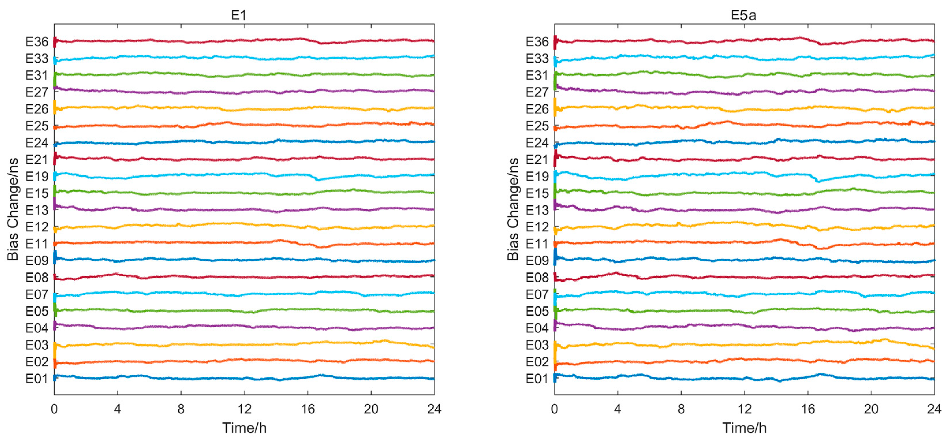
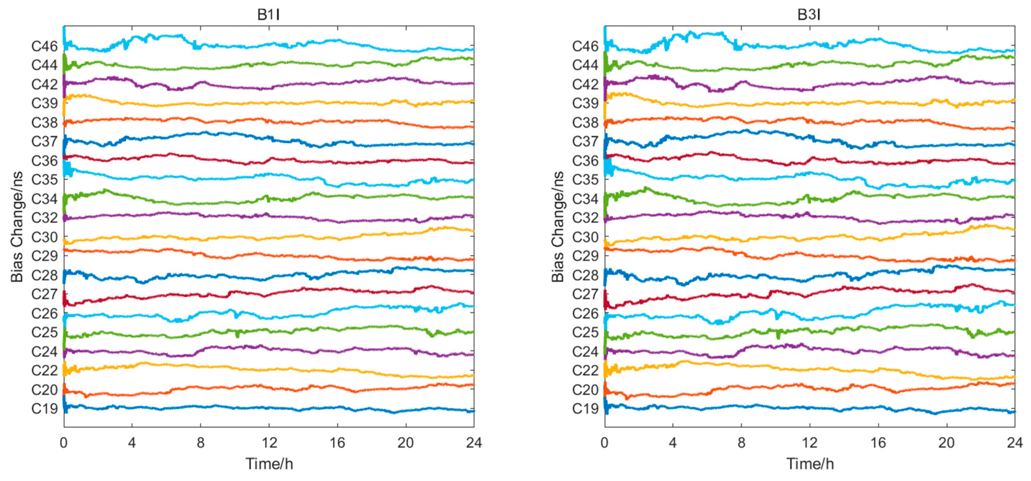
3.2. Analysis of Experimental Results for OSB Products

The multi-system OSB products were generated by the software developed by the Chinese Academy of Surveying and Mapping (CASM). The plots of the OSB products at all frequencies obtained by DOY 301 in 2021 are presented in Figure 3, Figure 4 and Figure 5; to distinguish satellites, they were arranged from bottom to top according to the satellite number, with 0.2 ns spacing between satellites. As shown in Figure 3 and Figure 4, the phase bias on each frequency of the GPS and Galileo systems varied relatively smoothly throughout the day. The E14 and E18 satellites were excluded from the OSB estimation since the number of epochs in the continuous arc segment did not reach the preset threshold. The average STD values for the L1 and L2 frequencies of all GPS satellites were 0.014 ns and 0.018 ns, respectively, as shown in

Table 2. Average STD values of the BDS-3/ GPS/ Galileo’s OSB for DOY 301, 2021.

System	BDS-3		GPS		Galileo
Frequency	B1I	B3I	L1	L2	E1	E5a
STD (ns)	0.035	0.043	0.014	0.018	0.014	0.019

; the average STD values for the E1 and E5a frequencies of the Galileo satellites were 0.014 ns and 0.019 ns, respectively. The average STD of the phase bias at each frequency was slightly larger for the BDS-3 system than for the other two systems. The average STD values for B1I and B3I frequencies were 0.035 ns and 0.043 ns, respectively. Overall, the stability of the phase bias products was significantly better than 0.05 ns at each frequency for all three systems.

The residual distribution of the FCB estimates was used as one of the criteria for testing the quality of the FCB product. Figure 6 and Figure 7 show the distributions of residuals for the GPS, Galileo, BDS-3 systems for the WL-and NL-FCBs, respectively. The probability that the residuals of the three systems’ WL-FCBs fall within ±0.25 cycles was better than 96%, indicating that most of the WL ambiguities could be reliably repaired. For the BDS-3, GPS, and Galileo systems, the percentage values of NL residuals within ±0.25 cycles were 96%, 97%, and 97%, and 94%, 95%, and 95% within ±0.15 cycles, respectively. In addition, the mean values of the residuals for all three systems were close to zero for both WL- and NL-FCBs, which further verified the reliability of the FCB results.

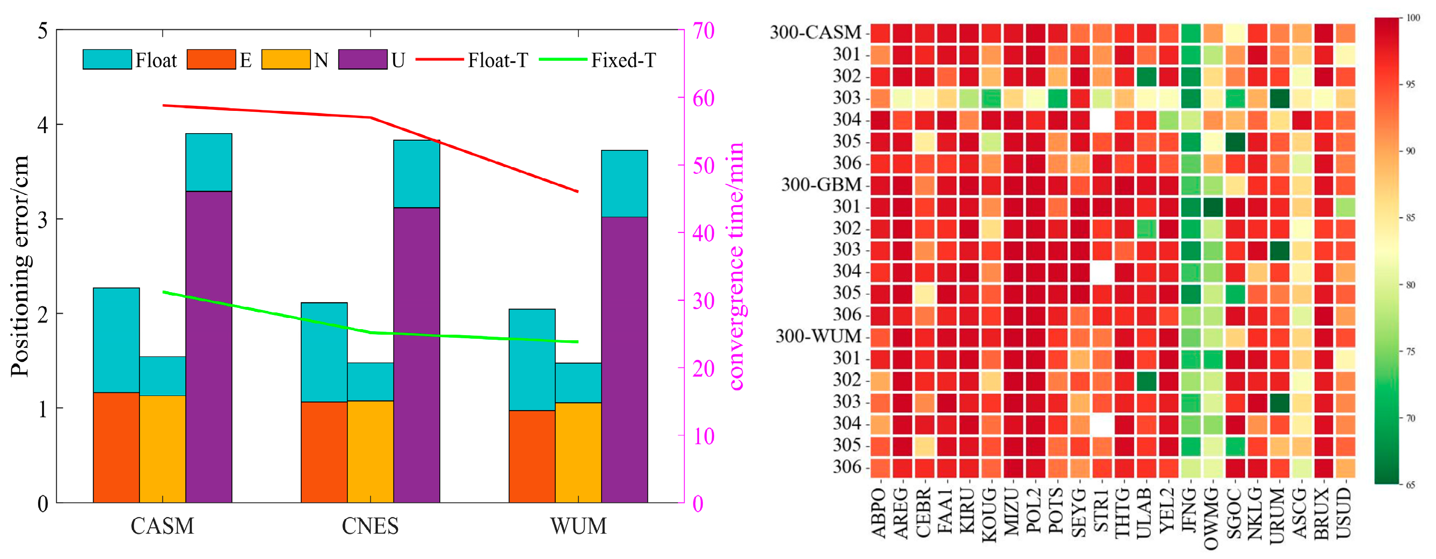
3.3. Analysis of Positioning Accuracy and Convergence Performance of Different Institutional Products

To verify the usability of the OSB products from the Chinese Academy of Surveying and Mapping (CASM), they were compared with the OSB products post-processed by the CNES (based on GFZ rapid orbit/clock solutions) and the OSB products provided by the PRIDE Lab at Wuhan University. For the purpose of brevity, “CASM_OSB”, “GBM_OSB”, and “WUM_OSB” denote the OSB products from the Chinese Academy of Surveying and Mapping, CNES, and PRIDE Lab, respectively. It should be noted that in PPP ambiguity resolution, the same precise orbit and clock products were used as on the service to ensure product consistency. The CASM_OSB product corresponded to the center for orbit determination in Europe’s (CODE) precise orbit and clock products, the GBM_OSB product corresponded to the GeoForschungsZentrum’s (GFZ) rapid orbit and clock products, and the WUM_OSB product corresponded to the precise orbit of the Wuhan Analysis Centre and precise clock products generated by the PRIDE Lab. Detailed information on the OSB products is shown in

Table 3. Overview of the OSB products (The websites were accessed on 20 April 2022).

Institution	Orbit	Clock	Website for OSB Products
CASM (CASM_OSB)	CODE’s precise orbit	CODE’s precise clock	Not released yet
CNES (GBM_OSB)	GFZ’s rapid orbit	GFZ’s rapid clock	ftp://ftp.ppp-wizard.net/PRODUCTS/POST_PROCESSED/ (accessed on 20 April 2022)
WUM (WUM_OSB)	WUM’s precise orbit	WUM_PRIDE’s precise clock	ftp://igs.gnsswhu.cn/pub/whu/phasebias/xxxx/bias/ (accessed on 20 April 2022)

.

This section compares in detail the differences in the PPP-AR for the OSB products of the three institutions. Figure 8 and Figure 9 show GPS static and kinematic average positioning errors for seven days at 22 stations using products from different institutions. In the static mode, daily observables were separated into six four-hour-long observable sessions for experiments. In addition, the average convergence time and the success rate of fixed ambiguity were also evaluated. The convergence time criterion adopted in this study referred to 20 consecutive epochs with fixed ambiguity and positioning accuracy of better than 10 cm in the E, N, and U directions. The fixed ambiguity success rate referred to the percentage rate of the number of epochs whose ambiguity was correctly fixed to the number of all epochs. Unless stated otherwise, results were evaluated based on the above assessment indicators. Due to the space limitation, only the float and fixed PPP solutions for the IF model are presented in this section.

Regardless of the mode type, static or kinematic mode, the PPP-AR of the OSB products of the three institutions could improve the accuracy of the PPP solution and shorten the convergence time. In addition, it was proved that the positioning accuracy of fixed-ambiguity PPP in the E direction was improved most significantly. Specifically, as shown in

Table 4. The RMS results of positioning error and convergence time of the GPS-only and GCE float/fixed PPP static (left) and kinematic (right) of different institutions on DOY 300-306, 2021, for 22 stations.

			Static				Kinematic
			E (cm)	N (cm)	U (cm)	T (min)	E (cm)	N (cm)	U (cm)	T (min)
G	CASM	Float	1.0	0.5	1.4	33.0	2.3	1.5	3.9	58.8
		Fixed	0.5	0.4	1.3	17.4	1.2	1.1	3.3	31.2
	CNES	Float	0.9	0.4	1.4	32.5	2.1	1.5	3.8	57.0
		Fixed	0.5	0.4	1.3	15.5	1.1	1.1	3.1	25.2
	WUM	Float	0.9	0.5	1.3	24.2	2.0	1.5	3.7	46.0
		Fixed	0.5	0.5	1.3	15.2	1.0	1.1	3.0	23.8
GCE	CASM	Float	0.7	0.5	1.4	15.5	1.4	0.9	2.9	22.9
		Fixed	0.4	0.4	1.3	7.8	0.8	0.8	2.7	16.4
	CNES	Float	0.7	0.4	1.4	14.0	1.5	1.0	3.1	21.5
		Fixed	0.5	0.4	1.3	9.0	0.8	0.8	2.7	16.0
	WUM	Float	0.7	0.5	1.3	13.5	1.3	0.9	2.7	18.3
		Fixed	0.4	0.4	1.3	6.0	0.7	0.7	2.3	15.5

, in GPS static mode, the CASM_OSB improved the E-direction by 50% (from 1.0 cm to 0.5 cm) and reduced the convergence time by 47% (from 33.0 min to 17.4 min). The GBM_OSB improved the E-direction by 44% (from 0.9 cm to 0.5 cm) and reduced the convergence time by 52% (from 32.5 min to 15.5 min). The WUM_OSB improved in the E-direction by 44% (from 0.9 cm to 0.5 cm) and reduced the convergence time by 37% (from 24.2 min to 15.2 min). The average fixed ambiguity success rates for the three institutions were 91%, 91%, and 91%; thus, they were all above 90%. In the GPS kinematic mode, the CASM_OSB improved the E-direction by 49% (from 2.3 cm to 1.2 cm) and reduced the convergence time by 47% (from 58.8 min to 31.2 min). The GBM_OSB improved the E-direction by 48% (from 2.1 cm to 1.1 cm) and reduced the convergence time by 56% (from 57.0 min to 25.2 min). Finally, the WUM_OSB improved in the E-direction by 50% (from 2.0 cm to 1.0 cm) and reduced the convergence time by 48% (from 46.0 min to 23.8 min). The average ambiguity fixed success rates for the three institutions were 93%, 94%, and 93%; they were all above 90%.

As shown in Table 4, the CASM’s OSB products were comparable in terms of performance to those of the CNES and WUM institutions and can be used in the user end PPP-AR.

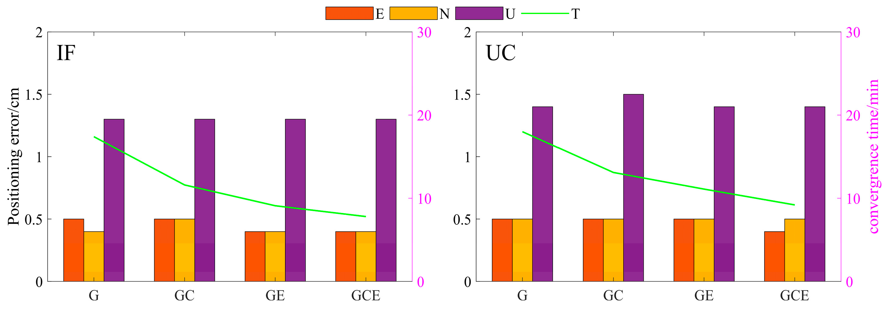
3.4. Comparative Analysis of Positioning Accuracy and Convergence Time Based on CASM’s Product under IF and UDUC Models

To illustrate the stability of different systems and positioning model CASM_OSB products for the PPP-AR, the static and kinematic positioning errors of the YEL2 station DOY 301 are presented in Figure 10 and Figure 11, respectively. In Figure 10 and Figure 11, the left panel shows the IF model, and the right panel shows the UDUC model. The results demonstrate that regardless of the used model, the IF model or the UDUC model, the GCE multi-system PPP-AR in the static and kinematic modes had the smoothest positioning accuracy, followed by the GE and GC, with a single GPS being worse than the first three. In the kinematic mode, the 3D RMS values corresponding to the IF models GCE, GE, GC, and G were 1.3 cm, 1.5 cm, 1.6 cm, and 1.6 cm, with the convergence times of 9.0 min, 12.0 min, 10.0 min, and 23.0 min, respectively. The 3D RMS values corresponding to the UDUC models GCE, GE, GC, and G were 1.3 cm, 1.5 cm, 1.5 cm, and 1.6 cm, with the convergence times of 8.5 min, 10.5 min, 14.0 min, and 25.0 min, respectively. In the static mode, the convergence times corresponding to the IF models GCE, GE, GC, and G were 2.8 min, 3.7 min, 4.3 min, and 6.0 min, respectively. The convergence times corresponding to UDUC models GCE, GE, GC, and G were 3.2 min, 3.7 min, 5.5 min, and 6.8 min, respectively. The convergence times of the GCE multi-system for the IF model and the UDUC model were both reduced by a factor of two compared to a single GPS system.

To analyze the advantages of different system IF models and the UDUC model PPP-AR further, seven-day data from all stations were processed to calculate the average solution for all stations and days. The PPP-AR positioning accuracy and convergence time for different systems’ IF and UDUC models were calculated. As shown in Figure 12 (static) and Figure 13 (kinematic), the PPP-AR positioning accuracy and convergence time results for different systems were comparable under both models. The GCE multi-system performed best in terms of both the positioning accuracy and the convergence time, and it was followed by the GE and GC systems, while the single-GPS performs worse than the dual (GC, GE) and triple (GCE) systems in terms of positioning accuracy and convergence time. The fixed ambiguity success rate has been one of the commonly used metrics for the evaluation of OSB product performance and positioning models. To save space, only the GCE system’s static and kinematic fixed ambiguity success rates for the IF model and the UDUC model are given in Figure 14 and Figure 15. The static mode was 95% and 95%, respectively; the kinematic mode was 97% and 96%, respectively, thus further demonstrating the equivalence of the IF model and the UDUC model under PPP-AR.

For quantitative analysis, the average positioning error and convergence time of the PPP and PPP-AR for different systems under the IF and UDUC models for both static and kinematic modes are given in

Table 5. The RMS results of position differences and convergence time of the IF model (left) and the UDUC model (right) G, GC, GE, and GCE static float/fixed PPP on DOY 300-306, 2021, for 22 stations.

		IF				UDUC
		E (cm)	N (cm)	U (cm)	T (min)	E (cm)	N (cm)	U (cm)	T (min)
G	Float	1.0	0.5	1.4	33.0	1.3	0.6	1.5	46.9
	Fixed	0.5	0.4	1.3	17.4	0.5	0.5	1.4	18.0
	Improvement (%)	51	13	6	47	61	17	10	62
GC	Float	0.8	0.5	1.5	19.8	0.9	0.6	1.6	29.9
	Fixed	0.5	0.5	1.3	11.6	0.5	0.5	1.5	13.1
	Improvement (%)	36	5	8	40	44	13	5	56
GE	Float	0.8	0.5	1.4	19.9	0.9	0.6	1.4	29.6
	Fixed	0.4	0.4	1.3	9.1	0.5	0.5	1.4	11.1
	Improvement (%)	52	14	4	54	50	16	5	62
GCE	Float	0.7	0.5	1.4	15.5	0.8	0.6	1.4	22.8
	Fixed	0.4	0.4	1.3	7.8	0.4	0.5	1.4	9.2
	Improvement (%)	45	14	5	50	45	17	4	60

and

Table 6. The RMS results of position differences and convergence time of the IF model (left) and the UDUC model (right) G, GC, GE, and GCE kinematic float/fixed PPP on DOY 300-306, 2021, for 22 stations.

		IF				UDUC
		E (cm)	N (cm)	U (cm)	T (min)	E (cm)	N (cm)	U (cm)	T (min)
G	Float	2.3	1.5	3.9	58.8	2.6	1.7	4.2	78.5
	Fixed	1.2	1.1	3.3	31.2	1.2	1.2	3.3	34.9
	Improvement (%)	49	27	16	47	54	30	22	56
GC	Float	1.5	1.1	3.2	31.3	1.7	1.3	3.4	49.1
	Fixed	1.0	1.0	3.0	17.7	1.1	1.1	3.2	20.3
	Improvement (%)	33	10	7	44	37	18	6	59
GE	Float	1.7	1.1	3.3	31.5	1.9	1.2	3.4	49.3
	Fixed	0.9	0.9	2.8	19.0	1.0	1.0	2.9	21.4
	Improvement (%)	49	18	14	40	47	20	15	57
GCE	Float	1.4	0.9	2.9	22.9	1.5	1.0	3.0	31.5
	Fixed	0.8	0.8	2.7	16.4	0.9	0.9	2.8	16.4
	Improvement (%)	40	16	9	28	38	11	8	48

, respectively.

Based on the results in Table 5 and Table 6, the following conclusions can be drawn:

(1)

For the PPP solution, the IF model provided slightly better positioning accuracy and convergence time than the UDUC model. This could be because the UDUC model needed to estimate ionospheric delay and had more parameters to be estimated than the IF model;

(2)

For the PPP fixed solution, the CASM OSB products could effectively improve the positioning accuracy and convergence time of the PPP when used in the PPP-AR. The most significant improvement in the positioning accuracy was observed in the E direction, with an average improvement of 46% for the IF model and 50% for the UDUC model in the static mode. The improvements under both models were above 45%. Further, for the IF model, the convergence time improved by an average of 48%, and for the UDUC model, an average improvement was 60%. In the kinematic mode, the localization accuracy under the IF model in the E direction improved by 43% on average, and that of the UDUC model improved by 44% on average; thus, they were both above 40%. The average improvements in the convergence time under the IF and UDUC models were 40% and 55%, respectively. Furthermore, an interesting conclusion was drawn: the IF model and the UDUC model PPP-AR had comparable positioning accuracy and convergence time.

(3)

The single-system fixed-ambiguity PPP solution showed more significant improvement compared to the PPP float solution. In the static mode, the average positioning accuracy improvements of the GPS system in the E, N, and U directions were 56%, 15%, and 8%, respectively. In the kinematic mode, the average positioning accuracy improvements of the GPS system in the E, N, and U directions were 52%, 28%, and 19%, respectively. Comparing the positioning accuracy and convergence time results of different system combinations showed that the GCE multi-system combination outperformed the other system combinations. Specifically, the average positioning accuracy in the E, N, and U directions for the static PPP fixed solution was 0.4 cm, 0.4 cm, and 1.4 cm, respectively, with an average convergence time of 8.5 min. The average positioning accuracy in the E, N, and U directions for the kinematic PPP fixed solution was 0.9 cm, 0.9 cm, and 2.8 cm, respectively, with an average convergence time of 16.4 min.

4. Discussion

According to the results, the CASM’s OSB products were comparable in terms of performance to those of the CNES and WUM institutions and can be used in the PPP-AR with different positioning models on the user end. Based on the results, the average STD of the OSB at each frequency for the GPS and Galileo systems varied relatively smoothly throughout the day. The average STD of the OSB at each frequency for the BDS-3 system was slightly larger compared to the GPS and Galileo systems, with an average STD of 0.035 ns and 0.043 ns for B1I and B3I frequencies, respectively. The BDS-3 system used the same strategy as the GPS and Galileo systems for the FCB estimation but did not consider the differences between the MEO and IGSO satellites of the BDS-3, and there was no PCV product correction in the BDS-3 system. In addition, the accuracy of satellite orbit and clock products could also be the reason for this phenomenon. As the number of stations available for observing BDS-3 satellites increased, the accuracy of the precise orbit and clock products of the BDS-3 satellites also increased. The accuracy of the OSB at each frequency of the BDS-3 system is expected to improve further due to the above possible reasons.

The IF model of the dual-frequency PPP solution had slightly better positioning accuracy and convergence time than the UDUC model, which could be due to the need for the UDUC model to estimate the ionospheric delay.

Although the UDUC model has many parameters to estimate, the PPP-AR’s positioning accuracy and convergence time are comparable to those of the IF model; also, the UDUC model can retain the ionospheric information. The estimated ionospheric information can be used for studying ionospheric modeling and inversion and differential code bias estimation. The current systems can broadcast observation information at three or even more frequencies, but the multi-frequency uncombined ambiguity fixed results could be even better.

5. Conclusions

The OSB can interact directly with the original observations, providing complete flexibility for the PPP-AR. In this study, the OSB estimation method is derived in detail. Moreover, the OSB product generation is performed for the GPS, Galileo, and BDS-3 systems, and its performance is evaluated using 117 globally distributed MGEX stations. In addition, a detailed theoretical derivation of the relationship between the UDUC and IF models is given, and a comparative analysis of the PPP-AR of the two positioning models is conducted.

The conclusions made based on the obtained results are as follows:

(1)

The stability of the CASM-generated OSB products is better than 0.05 ns and can be used for the PPP ambiguity resolution. For both static and kinematic modes, the GPS PPP-AR has comparable positioning accuracy and convergence time with the WUM and CNES, and the average fixed-ambiguity success rate is above 90% for all three institutions.

(2)

The IF model of the PPP solution has slightly better positioning accuracy and convergence time than the UDUC model. This could be because the UDUC model needs to estimate the ionospheric delay and has more parameters to estimate. However, the IF and UDUC models’ PPP-AR values have comparable positioning accuracy and convergence time. The CASM OSB products for the PPP-AR can effectively improve the positioning accuracy and convergence time of the PPP. The most significant improvement in positioning accuracy is achieved in the E direction, with an average improvement of more than 45% and 40% for both models in the static and kinematic modes, respectively. The convergence times of the IF and UDUC models are improved by an average of 48% and 60% in the static mode and by 40% and 55% in the kinematic mode, respectively.

(3)

The single system fixed-ambiguity PPP solution shows more significant improvement compared to the PPP float solution. The possible reason for this could be that the single system PPP float solution is less accurate than the dual- and multi-systems, resulting in a more significant fixed-ambiguity PPP solution. In the static mode, the average improvement in the GPS positioning accuracy in the E, N, and U directions is 56%, 15%, and 8%, respectively. Similarly, in the kinematic mode, the average improvement in the GPS positioning accuracy in the E, N, and U directions is 52%, 28%, and 19%, respectively.

(4)

Comparing the positioning accuracy and convergence time of different system combinations for PPP-AR shows that the GCE multi-system combination is superior to the other system combinations. Specifically, the average positioning accuracy in the E, N, and U directions for the static PPP fixed solution is 0.4 cm, 0.4 cm, and 1.4 cm, respectively, with an average convergence time of 8.5 min. The average positioning accuracy in the E, N, and U directions for the kinematic PPP fixed solution is 0.9 cm, 0.9 cm, and 2.8 cm, respectively, with an average convergence time of 16.4 min.

The proposed OSB estimation method can also be applied to the multi-frequency OSB generation, which could be investigated in future work. In addition, the multi-frequency UDUC PPP-AR could be further studied considering inter-frequency clock biases.

References

1. Geng, J.; Pan, Y.; Li, X.; Guo, J.; Liu, J.; Chen, X.; Zhang, Y. Noise Characteristics of High-Rate Multi-GNSS for Subdaily Crustal Deformation Monitoring. J. Geophys. Res. Solid Earth 2018, 123, 1987–2002. [Google Scholar] [CrossRef]
2. Su, K.; Jin, S.; Ge, Y. Rapid displacement determination with a stand-alone multi-GNSS receiver: GPS, Beidou, GLONASS, and Galileo. GPS Solut. 2019, 23, 54. [Google Scholar] [CrossRef]
3. Gao, Y.; Shen, X. A New Method for Carrier-Phase-Based Precise Point Positioning. Navigation 2002, 49, 109–116. [Google Scholar] [CrossRef]
4. Gao, Z.; Zhang, H.; Ge, M.; Niu, X.; Shen, W.; Wickert, J.; Schuh, H. Tightly coupled integration of multi-GNSS PPP and MEMS inertial measurement unit data. GPS Solut. 2017, 21, 377–391. [Google Scholar]
5. Chen, W.; Hu, C.; Li, Z.; Chen, Y.; Ding, X.; Gao, S.; Ji, S. Kinematic GPS precise point positioning for sea level monitoring with GPS. J. Glob. Position. Syst. 2004, 3, 302–307. [Google Scholar] [CrossRef]
6. Colombo, O.L.; Sutter, A.W.; Evans, A.G. Evaluation of precise, kinematic GPS point positioning. In Proceedings of the 17th International Technical Meeting of the Satellite Division (ION GNSS 2004), Long Beach, CA, USA, 21–24 September 2004; pp. 1423–1430. [Google Scholar]
7. Bisnath, S.; Gao, Y. Current state of precise point positioning and future prospects and limitations. In Proceedings of the IUGG 24th General Assembly, Perugia, Italy, 2–13 July 2007. [Google Scholar]
8. Rocken, C.; Johnson, J.; Hove, T.V.; Iwabuchi, T. Atmospheric water vapor and geoid measurements in the open ocean with GPS. Geophys. Res. Lett. 2005, 32, L12813. [Google Scholar] [CrossRef]
9. Satirapod, C. Stochastic Models used in Static GPS Relative Positioning. Surv. Rev. 2006, 38, 379–386. [Google Scholar] [CrossRef]
10. Teferle, F.N.; Orliac, E.J.; Bingley, R.M. An assessment of Bernese GPS software precise point positioning using IGS final products for global site velocities. GPS Solut. 2007, 11, 205–213. [Google Scholar] [CrossRef]
11. Zhang, X.; Andersen, O.B. Surface ice flow velocity and tide retrieval of the Amery ice shelf using precise point positioning. J. Geod. 2007, 80, 171–176. [Google Scholar]
12. Geng, T.; Su, X.; Fang, R.; Xie, X.; Zhao, Q.; Liu, J. BDS Precise Point Positioning for Seismic Displacements Monitoring: Benefit from the High-Rate Satellite Clock Corrections. Sensors 2016, 16, 2192. [Google Scholar] [CrossRef]
13. Ge, M.; Gendt, G.; Rothacher, M.; Shi, C.; Liu, J. Resolution of GPS carrier-phase ambiguities in Precise Point Positioning (PPP) with daily observations. J. Geod. 2008, 82, 389–399. [Google Scholar] [CrossRef]
14. Geng, J.; Meng, X.; Teferle, F.N.; Dodson, A.H. Performance of precise point positioning with ambiguity resolution for 1-to 4-hour observation periods. Surv. Rev. 2010, 42, 155–165. [Google Scholar] [CrossRef] [Green Version]
15. Teunissen, P.J.G. The least-squares ambiguity decorrelation adjustment: A method for fast GPS integer ambiguity estimation. J. Geod. 1995, 70, 65–82. [Google Scholar] [CrossRef]
16. Zhang, X.; Li, P. Assessment of correct fixing rate for precise point positioning ambiguity resolution on a global scale. J. Geod. 2013, 87, 579–589. [Google Scholar] [CrossRef]
17. Laurichesse, D.; Mercier, F.; Berthias, J.P.; Broca, P.; Cerri, L. Integer ambiguity resolution on undifferenced GPS phase measure-ments and its application to PPP and satellite precise orbit determination. Navigation 2009, 56, 135–149. [Google Scholar] [CrossRef]
18. Collins, P.; Bisnath, S.; Lahaye, F.; Héroux, P. Undifferenced GPS ambiguity resolution using the decoupled clock model and ambiguity datum fixing. Navigation 2010, 57, 123–135. [Google Scholar] [CrossRef]
19. Geng, J.; Meng, X.; Dodson, A.H.; Teferle, F.N. Integer ambiguity resolution in precise point positioning: Method comparison. J. Geod. 2010, 84, 569–581. [Google Scholar] [CrossRef]
20. Shi, J.; Gao, Y. A comparison of three PPP integer ambiguity resolution methods. GPS Solut. 2014, 18, 519–528. [Google Scholar] [CrossRef]
21. Geng, J.; Guo, J.; Chang, H.; Li, X. Towards global instantaneous decimeter-level positioning using tightly-coupled multi-constellation and multi-frequency GNSS. J. Geod. 2019, 93, 977–991. [Google Scholar] [CrossRef]
22. Qi, K.; Dang, Y.; Xu, C.; Gu, S. An Improved Fast Estimation of Satellite Phase Fractional Cycle Biases. Remote Sens. 2022, 14, 334. [Google Scholar] [CrossRef]
23. Xiao, G.; Sui, L.; Heck, B.; Zeng, T.; Tian, Y. Estimating satellite phase fractional cycle biases based on Kalman filter. GPS Solut. 2018, 22, 1–2. [Google Scholar] [CrossRef]
24. Cai, C.; Gao, Y. Modeling and assessment of combined GPS/GLONASS precise point positioning. GPS Solut. 2013, 17, 223–236. [Google Scholar] [CrossRef]
25. Li, X.; Ge, M.; Zhang, H.; Nischan, T.; Wickert, J. The GFZ real-time GNSS precise positioning service system and its adaption for COMPASS. Adv. Space Res. 2013, 51, 1008–1018. [Google Scholar] [CrossRef]
26. Li, X.; Ge, M.; Dai, X.; Ren, X.; Fritsche, M.; Wickert, J.; Schuh, H. Accuracy and reliability of multi-GNSS real-time precise positioning: GPS, GLONASS, BeiDou, and Galileo. J. Geod. 2015, 89, 607–635. [Google Scholar] [CrossRef]
27. Li, X.; Zhang, X.; Ren, X.; Fritsche, M.; Wickert, J.; Schuh, H. Precise positioning with current multi-constellation Global Navigation Satellite Systems: GPS, GLONASS, Galileo and BeiDou. Sci. Rep. 2015, 5, 8328. [Google Scholar] [CrossRef] [PubMed]
28. Shi, C.; Yi, W.; Song, W.; Lou, Y.; Yao, Y.; Zhang, R. GLONASS pseudorange inter-channel biases and their effects on combined GPS/GLONASS precise point positioning. GPS Solut. 2013, 17, 439–451. [Google Scholar]
29. Geng, J.; Shi, C. Rapid initialization of real-time PPP by resolving undifferenced GPS and GLONASS ambiguities simultaneously. J. Geod. 2016, 91, 361–374. [Google Scholar] [CrossRef]
30. Yi, W.; Song, W.; Lou, Y.; Shi, C.; Yao, Y.; Guo, H.; Chen, M.; Wu, J. Improved method to estimate undifferenced satellite fractional cycle biases using network observations to support PPP ambiguity resolution. GPS Solut. 2017, 21, 1369–1378. [Google Scholar] [CrossRef]
31. Liu, Y.; Ye, S.; Song, W.; Lou, Y.; Gu, S. Rapid PPP ambiguity resolution using GPS+ GLONASS observations. J. Geod. 2017, 91, 441–455. [Google Scholar] [CrossRef]
32. Li, P.; Zhang, X.; Guo, F. Ambiguity resolved precise point positioning with GPS and BeiDou. J. Geod. 2017, 91, 25–40. [Google Scholar]
33. Liu, Y.; Ye, S.; Song, W.; Lou, Y.; Chen, D. Integrating GPS and BDS to shorten the initialization time for ambiguity-fixed PPP. GPS Solut. 2017, 21, 333–343. [Google Scholar] [CrossRef]
34. Tegedor, J.; Liu, X.; Jong, K.; Goode, M.; Øvstedal, O.; Vigen, E. Estimation of Galileo Uncalibrated Hardware Delays for Ambiguity-Fixed Precise Point Positioning. Navigation 2016, 63, 173–179. [Google Scholar] [CrossRef]
35. Xiao, G.; Li, P.; Sui, L.; Heck, B.; Schuh, H. Estimating and assessing Galileo satellite fractional cycle bias for PPP ambiguity resolution. GPS Solut. 2018, 23, 3. [Google Scholar] [CrossRef]
36. Li, X.; Li, X.; Yuan, Y.; Zhang, K.; Zhang, X.; Wickert, J. Multi-GNSS phase delay estimation and PPP ambiguity resolution: GPS, BDS, GLONASS, Galileo. J. Geod. 2017, 92, 579–608. [Google Scholar] [CrossRef]
37. Schaer, S. SINEX_BIAS-Solution (Software/technique) Independent Exchange Format for GNSS Biases Version 1.00. In Proceedings of the IGS Workshop on GNSS Biases, Bern, Switzerland, 5–6 November 2015. [Google Scholar]
38. Villiger, A.; Schaer, S.; Dach, R.; Prange, L.; Sušnik, A.; Jäggi, A. Determination of GNSS pseudo-absolute code biases and their long-term combination. J. Geod. 2019, 93, 1487–1500. [Google Scholar] [CrossRef]
39. Laurichesse, D.; Banville, S. Instantaneous Centimeter-Level Multi-Frequency Precise Point Positioning. GPS World, Innovation Column, 4 July 2018. Available online: www.gpsworld.com/innovation-instantaneous-centimeter-level-multi-frequency-precise-point-positioning/ (accessed on 12 August 2021).
40. Banville, S.; Geng, J.; Loyer, S.; Schaer, S.; Springer, T.; Strasser, S. On the interoperability of IGS products for precise point positioning with ambiguity resolution. J. Geodesy. 2020, 94, 1–5. [Google Scholar] [CrossRef]
41. Liu, G.; Guo, F.; Wang, J.; Du, M.; Qu, L. Triple-frequency GPS un-differenced and uncombined PPP ambiguity resolution using observable-specific satellite signal biases. Remote Sens. 2020, 12, 2310. [Google Scholar] [CrossRef]
42. Liu, T.; Jiang, W.; Laurichesse, D.; Chen, H.; Liu, X.; Wang, J. Assessing GPS/Galileo real-time precise point positioning with ambiguity resolution based on phase biases from CNES. Adv. Space Res. 2020, 66, 810–825. [Google Scholar] [CrossRef]
43. Kouba, J. A Guide to Using International GNSS Service (IGS) Products. Available online: https://kb.igs.org/hc/en-us/articles/201271873-A-Guide-to-Using-the-IGS-Products (accessed on 12 August 2021).
44. Zhou, F. Theory and Methodology of Multi-GNSS Undifferenced and Uncombined Precise Point Positioning. Ph.D. thesis, East China Normal University, Shanghai, China, 2018. Ph.D. Thesis, East China Normal University, Shanghai, China, 2018. [Google Scholar]
45. Yang, Y. The Principle of Equivalent Weight: The Robust Least Squares Solution of Uniformity Model of the Parameter Adjustment. Bull. Surv. Mapp. 1994, 49, 33–35. [Google Scholar]
Figure 1. The flowchart of the OSB estimation and PPP-AR.
Remotesensing 14 04207 g001
Figure 2. Distribution of MGEX stations used for the server-end OSB estimation and user-end PPP-AR verification. Blue dots denote the reference stations used in the OSB estimation; red triangular dots denote the reference stations used for the PPP-AR verification at the user end.
Remotesensing 14 04207 g002
Figure 3. Time series of the observable-specific signal bias at L1 and L2 frequencies of the GPS for DOY 301, 2021.
Remotesensing 14 04207 g003
Figure 4. Time series of the observable-specific signal bias at E1 and E5a frequencies of the Galileo for DOY 301, 2021.
Remotesensing 14 04207 g004
Figure 5. Time series of the observable-specific signal bias at B1I and B3I frequencies of the BDS-3 for DOY 301, 2021.
Remotesensing 14 04207 g005
Figure 6. The WL residual distributions of the BDS-3, GPS, and Galileo on DOY 301, 2021.
Remotesensing 14 04207 g006
Figure 7. The NL residual distributions of the BDS-3, GPS, and Galileo on DOY 301, 2021.
Remotesensing 14 04207 g007
Figure 8. The GPS static RMS of positioning error, convergence time (left), and fixed-ambiguity success rate (right) on DOY 300–306, 2021, for 22 stations of the IF model for the CASM_OSB, GBM_OSB, and WUM_OSB products.
Remotesensing 14 04207 g008
Figure 9. The GPS kinematic RMS of positioning error, convergence time (left) and fixed-ambiguity success rate (right) on DOY 300–306, 2021, for 22 stations of the IF model for the CASM_OSB, GBM_OSB, and WUM_OSB products.
Remotesensing 14 04207 g009
Figure 10. The RMS results of position differences of the IF model (left) and UDUC model (right) G/GE/GC/GCE static PPP-AR on DOY 301, 2021, for the YEL2 station.
Remotesensing 14 04207 g010
Figure 11. The RMS results of position differences of the IF model (left) and UDUC model (right) G/GE/GC/GCE kinematic PPP-AR on DOY 301, 2021, for the YEL2 station.
Remotesensing 14 04207 g011
Figure 12. The RMS results of positioning error and convergence time of the IF model (left) and the UDUC model (right) G, GE, GC, and GCE static PPP-AR on DOY 300–306, 2021, for 22 stations.
Remotesensing 14 04207 g012
Figure 13. The RMS results of positioning error and convergence time of the IF model (left) and the UDUC model (right) G, GE, GC, and GCE kinematic PPP-AR on DOY 300–306, 2021, for 22 stations.
Remotesensing 14 04207 g013
Figure 14. The fixed-ambiguity success rate of GCE static PPP for the IF model and the UDUC model on DOY 300–306, 2021, for 22 stations.
Remotesensing 14 04207 g014
Figure 15. The fixed-ambiguity success rate of GCE kinematic PPP for the IF model and the UDUC model on DOY 300–306, 2021, for 22 stations.
Remotesensing 14 04207 g015