Abstract
Landslide susceptibility evaluation is critical for landslide prevention and risk management. Based on the slope unit, this study uses the information value method- random forest (IV-RF) model to evaluate the landslide susceptibility in the deep valley area. First, based on the historical landslide data, a landslide inventory was developed by using remote sensing technology (InSAR and optical remote sensing) and field investigation methods. Twelve factors were then selected as the input data for a landslide susceptibility model. Second, slope units with different scales were obtained by the r.slopeunits method and the information value method- random forest (IV-RF) model is used to evaluate the landslide susceptibility. Finally, the spatial distribution characteristics of landslide susceptibility grade under the optimal scale are analyzed. The results showed that under the slope unit obtained when c = 0.1 and a = 3 × 10⁵ m2, the internal homogeneity/external heterogeneity of 8425 slope units extracted by the r.slopeunits method is the best, with an AUC of 0.905 and an F1 of 0.908. In this case, the accuracy of landslide susceptibility evaluation is the highest as well; it is shown that the finer slope units would not always lead to the higher accuracy of landslide susceptibility evaluation results; it is necessary to comprehensively consider the internal homogeneity and external heterogeneity of the slope units. Under the optimal slope unit scale, the number of landslides in the highly and extremely highly susceptible areas in the landslide susceptibility map accounted for 82.60% of the total number of landslides, which was consistent with the actual distribution of landslides; this study shows that the method, combining the slope unit and the information value method- random forest (IV-RF) model, for landslide susceptibility evaluation can obtain high accuracy.
1. Introduction
Landslides are one of the most widely distributed and most serious types of geological disasters [1,2]. In recent years, global warming, extreme weather events, frequent earthquakes, and increasing human construction activities have caused landslides to occur more frequently, which resulted in large numbers of casualties and enormous economic loss [3,4,5,6]. Therefore, the quantitative evaluation of landslide susceptibility is of great significance.
Variations in mapping units may lead to different results in the analysis of landslide susceptibility [7,8,9]. Currently, the most widely applied mapping units include grid and slope units. A grid unit is in a regular rectangular shape with data is stored in rectangles, making it convenient for calculation and processing [10,11,12]. A slope unit, an area formed by a watershed line (or ridge line) and a discharge line (a valley line), is a basic topographical unit used for landslides [13,14,15]. A difference in mapping units can lead to different mapping results, thereby affecting the prediction accuracy of the analysis of regional landslide susceptibility [16,17]. The optimal grid unit scale in landslide susceptibility mapping has been extensively studied in recent years; however, the grid unit is not closely related to the actual geological environment where landslides occurred, which may result in a failure to predict landslide susceptibility accurately [18,19,20]. In contrast, a slope unit is closely related to the geological and geomorphological of landslides; however, the complexity in extracting slope units means that few studies have addressed the optimal slope units in regional landslide susceptibility mapping. Hence, it is necessary to carry out landslide susceptibility mapping based on the optimal slope unit.
Landslide susceptibility mapping models can be divided into three categories: empirical, statistical, and machine learning models. The empirical model includes the analytic hierarchy process (AHP) [21] and fuzzy mathematics methods [22]. The disadvantage of empirical methods is that they are subjective. The statistical model includes the certainty factor (CF) method [23], the information value method [24,25], the weight-of-evidence (WOE) method [26,27] and the frequency ratio method [28]. The disadvantage of statistical methods is that they cannot solve the non-linear relationship in the landslide factors. A machine learning model has a strong ability to learn; common methods include a support vector machine (SVM) [10,12], decision tree (DT) [29], random forest (RF) [30,31,32,33], and an artificial neural network (ANN) [11,34]. In recent years, the combination of statistical and machine learning models has been widely used in landslide susceptibility mapping [35,36,37,38]. The combination of different models can not only optimize the results and accuracy of model prediction, but also ensure the stability of model prediction in alpine valley areas with complicated topographical and geological structures along with frequent seismic activities.
In this study, it is assumed that on the basis of selecting the optimal slope unit scale, the information random forest (IV-RF) model has high accuracy in landslide sensitivity assessment in deep valley area. In order to verify this hypothesis, Maoxian County, located in the strong tectonic activity zone on the eastern margin of the Qinghai Tibet Plateau, is taken as the study area. Maoxian County, located in the strong tectonic activity zone on the eastern margin of the Qinghai-Tibet Plateau, is selected as the research area. Considering automatic slope unit partition and the homogeneity of the internal slope aspect and slope gradient. used the r.slopeunits method [17] to extract slope units of different scales and carried out landslide susceptibility mapping based on an information value-random forest (IV-RF) model. The results can provide a theoretical basis for landslide prevention and risk management.
2. Materials and Methods
2.1. Study Area
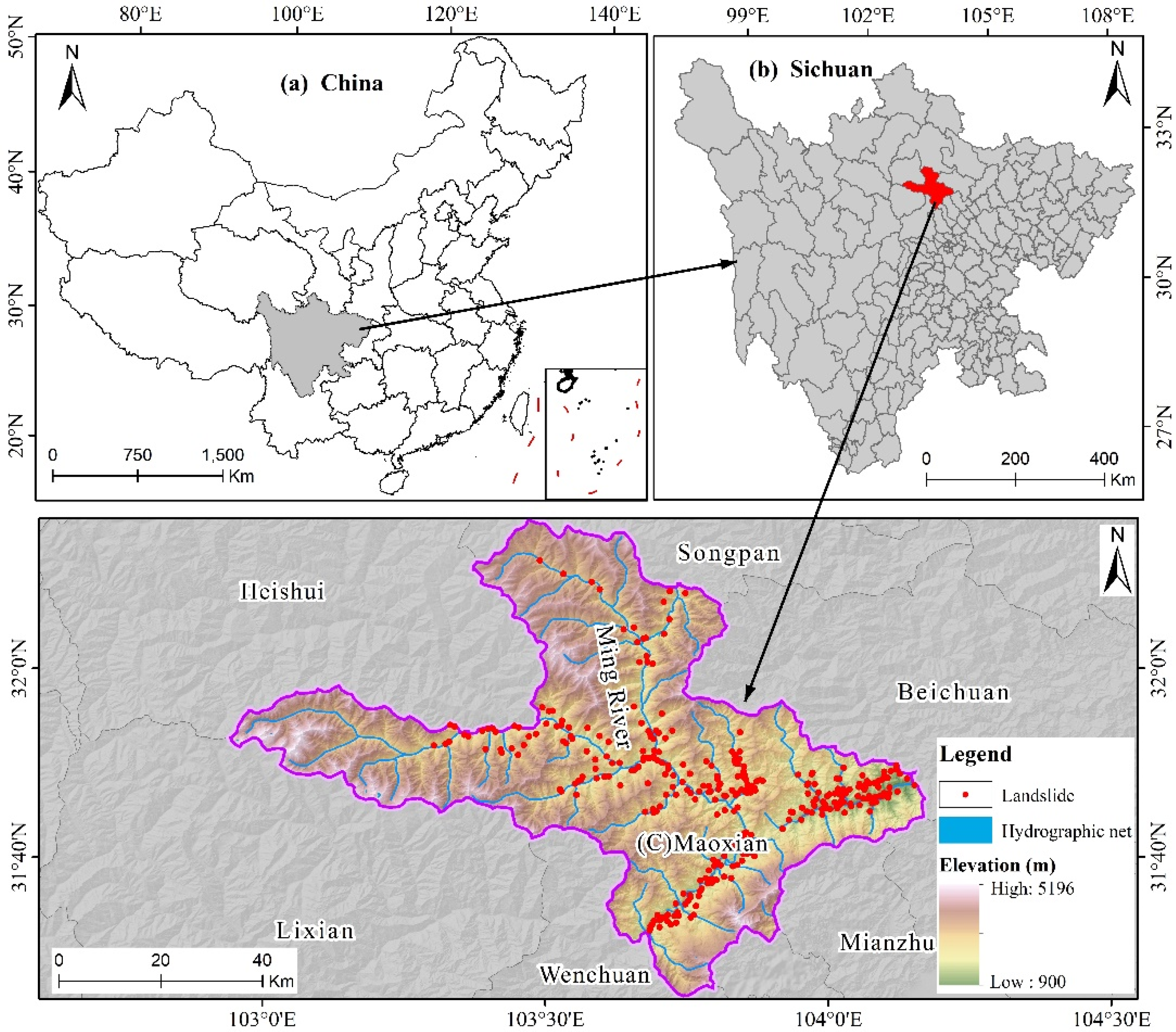
Located in the middle of the upper reaches of the Minjiang River valley and the southeastern rim of the Qinghai-Tibet Plateau (102°56′26″–104°10′32″E and 31°25′06″–32°15′43″N), Maoxian County covers an area of 3903 km2. Most of the area lies within the Qionglai and Minshan mountain ranges, and the southeastern part of the area is in the tail section of the Longmen Mountains. Maoxian County is covered by undulating hills, ridges and peaks, steep valley slopes, narrow river valleys and incised rivers with an average elevation of 3021 m (Figure 1).
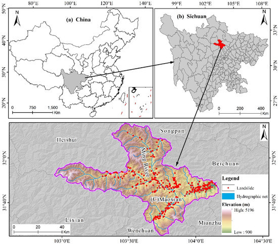
Figure 1.
Maps of the study area: (a) Location within China; (b) Location within Sichuan Province; (c) Locations and distribution of landslides in the study area.
Maoxian County has a monsoon climate with annual precipitation of 486.3 mm; rainfall from May to October accounts for over 80% of the annual precipitation. The maximum daily precipitation is 75.2 mm. The precipitation increases with an increase in elevation [39]; this county is located in the Minjiang and Tuojiang river systems and includes the main stream of Minjiang River and its tributary, the Heishui River, as well as the Tumen River of the Tuojiang river system.
The strata in the study area were laid down during the Triassic, Permian, Carboniferous, Devonian, Silurian (Maoxian group), Ordovician and Cambrian geological periods; the lithology is mainly phyllite and slate. The geological structure in the study area is mainly composed of the Jiaochang epsilon-type, the Shidaguan arc-shaped and the Longmenshan Cathaysian tectonic zones. The area also has multiple active faults, including Maoxian-Wenchuan, Shidaguan and Jiudingshan faults; these faults cause geological characteristics such as lithologic fracture and inverted attitude of strata in the area [40]. Located in the middle section of the north-south seismic belt, i.e., the Longmenshan and Songpan seismic belts, earthquakes occur frequently. The strongest earthquake in the area was the 7.5-magnitude Diexi earthquake in 1933.
2.2. Data
2.2.1. Landslide Inventory
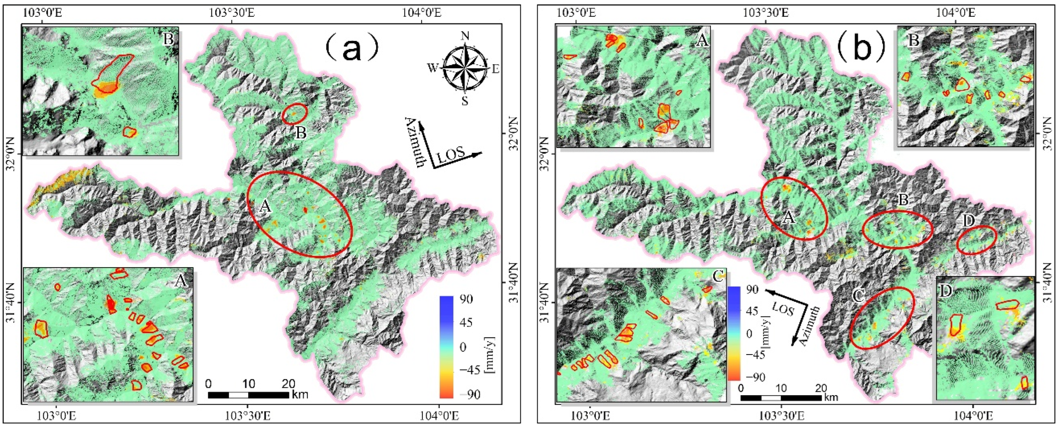
As an important basis for landslide susceptibility analysis, the accuracy of landslide inventory data directly affects the reliability of the results [41]. Therefore, the higher the accuracy and completeness of a landslide survey, the better the results of landslide susceptibility mapping. A reliable landslide inventory was obtained using multiple methods in the present study, including historical landslide data, Gaofen-2 satellite images of the study area acquired in 2020 (spatial resolution: 1 m), and Google Earth images acquired in 2011. A total of 297 historical landslides were obtained through a detailedinvestigation of geological hazards. Through the visual interpretation of landslides from Gaofen-2 image in 2020 (spatial resolution of 1 m) and Google Earth image in 2011, combined with field verification, 14 new landslides were obtained through optical remote sensing interpretation. In addition, using Small Baseline Subset Interferometric Synthetic Aperture Radar (SBAS-InSAR) technology [42,43], 68 landslides with continuous deformation were identified based on 61 ascending and 59 descending orbit scenes acquired by the Sentinel-1A satellite in the study area from January 2019 to December 2020, including 31 landslides identified in the ascending orbit, 41 in the descending orbit and four landslides found in both ascending and descending orbits (Figure 2). Through field verification of 68 landslides, 49 of them are historical landslide points, 14 of them coincide with the landslides interpreted by optical remote sensing, and 5 new landslides are obtained through SBAS-InSAR technology. Using the above methods, a total of 316 landslides were identified (Figure 3). In this study, the IVs of landslide factors were input into the RF model, which then output the significance of various factors and a landslide susceptibility index. According to the principles of the model, the same number of positive (landslide point: 1) and negative samples (non-landslide point: 0) should be chosen and divided into a testing set and a training set while using an appropriate ratio. A total of 316 non-landslide points were randomly chosen from the study area about 1 km away from the landslide points. The landslide and non-landslide points were randomly divided into a testing set (70%) and a training set (30%).
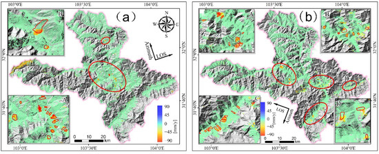
Figure 2.
InSAR identifies the distribution of landslides: (a) Average annual deformation rate from ascending orbits of the Sentinel-1A satellite (landslides are concentrated in A and B); (b) Average annual deformation rate from descending orbits of the Sentinel-1A satellite (landslides are concentrated in A, B, C and D).
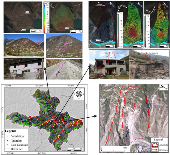
Figure 3.
Landslide distribution and presentation of typical landslides in the study area (Gaofen-2 base map).
2.2.2. Landslide Causes
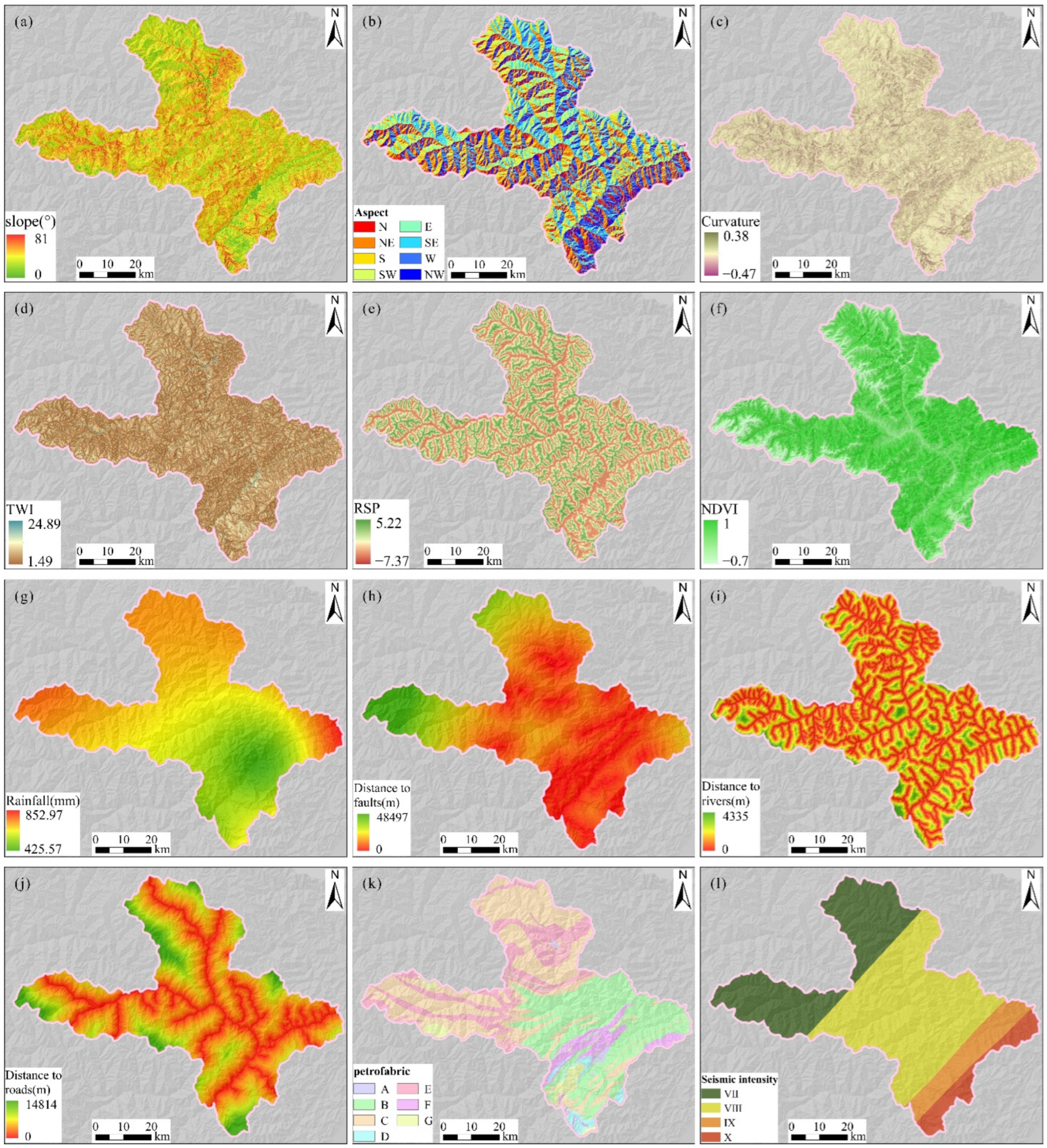
The selection of appropriate factors is the key to building a landslide susceptibility mapping model [44]. Common important factors include earthquakes, topography (lithologic and geological structure), hydrological factors, and human activities. According to the actual conditions of the study area, 12 factors, i.e., seismic intensity, engineering strata, geological structure, slope gradient, slope aspect, curvature, topographic wetness index (TWI), relative slope position (RSP), distance from the nearest river, distance from the nearest road, mean annual precipitation, and normalized difference vegetation index (NDVI) were chosen in this study to build the landslide susceptibility mapping model (Figure 4). According to the characteristics of each factor, slope aspect, engineering strata and seismic intensity were discrete variables, and the other factors were continuous variables.
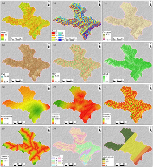
Figure 4.
Grid map of the evaluation factors in the study area: (a) Slope gradient; (b) slope aspect; (c) Curvature; (d) topographic wetness index (TWI); (e) relative slope position (RSP); (f) normalized difference vegetation index (NDVI); (g) Rainfall; (h) Distance to faults; (i) Distance to rivers; (j) Distance to Roads; (k) Petrofabric; (l) Seismic intensity.
The slope gradient is an important factor that affects the stability of a slope and directly determines the distribution of stress. The slope aspect determines how the local ground surface receives sunlight and redistributes solar radiation, which is directly related to the differences in the local microclimate of an area, thus affecting the vegetation as well as soil moisture and eventually affecting the stability of the slope. Slope curvature determines whether the surface flow flowing through the grid converges or becomes diffuse, thereby affecting the stability of the slope.
As an important topographical attribute, TWI also has a certain influence on landslides [45]; it is defined as the natural logarithm of the specific catchment area (SCA) to the tangent value of surface slope gradient (tanβ):
where, TWI is the topographic wetness index, and SCA is the upstream catchment area of the surface water in a unit length of the contour.
Relative slope position (RSP) is the relative position of the slope to the valley and ridge, which is calculated using Equation (2):
where RSP is the relative slope position (range: 0–1), z(s) is the elevation of the slope, and and are elevations of the valley and the ridge, respectively. The higher the RSP is, the closer to the ridge.
Slope gradient (°), slope aspect, curvature (m−1), TWI and RSP were extracted using SAGA GIS software with a digital elevation model (DEM) from the Advanced Land Observing Satellite (12.5 m).
Data related to two geological factors, lithology and faults, were obtained by vectorization of a 1:200,000 geological map. Faults and engineering petrofabrics are internal causes of landslides. The physical and mechanical parameters of different lithologies vary widely, resulting in different strengths in various slopes. Generally, the rock and earth mass in a fault zone are fragmentized, which will directly affect the stability of a side slope. The study area was divided into seven types of engineering petrofabrics based on the type of lithology present. The distance from the study area to a fault was obtained based on distance analysis.
Earthquakes are an important driving factor for landslides. Areas of high seismic intensity have a high probability of experiencing large-scale landslides [46]. The study area spans four seismic intensities (VII, VIII, IX and X), with VIII being the most frequent. Scouring of river systems and slope cutting for road repairs can lead to slope instability. Graphs of the distances to rivers and roads to the study area were obtained from ArcGIS vector quantization.
Precipitation is another important factor that affects landslides. Rainfall often infiltrates into a slope and increases the weight of the slope, saturating and softening the soil that is subject to sliding, and reducing its shearing strength and sliding resistance [47,48]. The mean annual precipitation data were obtained using Kriging interpolation of data obtained at seven meteorological stations. The NDVI is an index that reflects the surface vegetation coverage, which is calculated as follows:
where IR and R represent the measured reflectivity of the red and near-infrared spectra, respectively. An NDVI graph of the study area was obtained from Sentinel-2 satellite imagery with a cloud amount of less than 2% in 2020 using Google Earth Engine software.
2.3. Methods
A flow chart of the work in this study was divided into six stages (Figure 5): (1) A landslide inventory was established by integrating data collected by multiple types of remote sensing technology; (2) The K-Means clustering method was used to discretize the causes for continuous landslides; (3) Different scales of slope units were extracted using the r.slopeunits method; (4) Landslide susceptibility mapping was carried out under different slope unit scales based on an information value-random forest (IV-RF) model; (5) The optimal slope unit scale was determined based on the global aspect variance (V), global weighted Moran’s index, AUC and F1 values, and; (6) A landslide susceptibility map using the optimal slope unit was obtained.
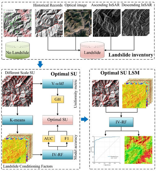
Figure 5.
Flow chart of the proposed method in this study.
2.3.1. Mapping Unit
The selection of mapping units was used as the basis for evaluating regional landslide stability. Considering automatic slope unit partitioning and the homogeneity of the internal slope aspect, the r.slopeunits method was used to extract the slope units [17].
In most landslide stability analyses, researchers assume that the units (i.e., internal slope aspect, slope gradient, mechanical parameters) are homogeneous [15,49,50]. Therefore, the maximum internal homogeneity and the maximum heterogeneity between units should be guaranteed during regional landslide susceptibility mapping based on slope units. The circular variance (c) controls the slope uniformity of slope units in the r.slopeunits method; thus, the global aspect variance (V) and global slope weighted Moran’s index (wMI) were used to represent the global heterogeneity of slope units [51]. The definitions are as follows:
where k is the total number of slope units, S is the total area, is the area of the ith slope unit, and is the variance of slope aspect of the ith slope unit. The smaller the V value is, the better the slope uniformity.
Moran’s index is often used to measure the heterogeneity between objects. Over- and under-division of slope units have a great impact on Moran’s Index (MI); thus, the global weighted Moran’s index (wMI) was used in this study:
where is the mean slope aspect of the ith slope unit, is the mean slope aspect of the entire study area, represents the spatial adjacency relationship of slope units. In this equation, = 1 or = 0 when the units are or not adjacent, respectively. The smaller the value of is, the lower the spatial correlation of the adjacent SU space is, and the stronger the heterogeneity is.
A good partition should lead to low intra-object variance (i.e., low intra-object heterogeneity) and low inter-object Moran’s index (i.e., high inter-object heterogeneity). The global heterogeneity measurement needs to take into account these two indices. In order to balance the intra- and inter-object heterogeneity measurements, the measurements were normalized:
where, , , and are the maximum and minimum values of the two indices at different scales. The smaller the GH value is, the better the partitioning result is.
2.3.2. K-Means Clustering
K-Means clustering is an unsupervised learning method that finds the optimal clustering center through multiple iterations such that the sum of the distance between the eigenvalue of each sample and the mean value is minimal [52]:
where is the eigenvalue of sample point x, is the mean value of the jth characteristic, is the collection of the jth type sample points after i iterations, and c is the number of categories.
The natural breakpoint method is often used in the grade classification of factors in traditional landslide susceptibility mapping models. The method is subjective and easily ignores the internal characteristics of units for interlaced topographical factors. Therefore, the K-Means clustering method was used to discretize the continuous factors in slope units to handle factors with interlaced geographical space. As for the discrete factors, the type with the largest proportion of slope units was taken as the slope unit factor. The steps of K-Means clustering are as follows:
(1) Calculate the mean value (MEAN) and standard deviation (STD) for the continuous factors in each slope unit.
(2) The MEAN and STD are input into the K-Means clustering method. The slope aspect, curvature, TWI, RSP, NDVI, mean annual precipitation, distance to the fault, distance to the river, distance to the road, initial number of clustering centers were set to 5, 3, 5, 5, 5, 5, 5, 6 and 5, respectively. Areas with similar topography were classified into the same category.
2.3.3. Information Value (IV) Model
As one of the Bayesian probability models, the information value model [53] presents a quantitative description in the form of a probability, which reflects the contribution of different disaster element intervals to the formation of geological disasters. The expression of geological disaster IV IAj→B is as follows:
where IAj→B represents the IV of geological disaster B in interval j of the disaster element A, n is the number of secondary intervals of disaster element A, Nj is the area of a geological disaster or the number of disaster points in interval j of disaster element A, Sj is the distribution area of interval j of disaster element A, N is the total distribution area or total points of regional geological disasters, and S is the total area.
2.3.4. Random Forest (RF)
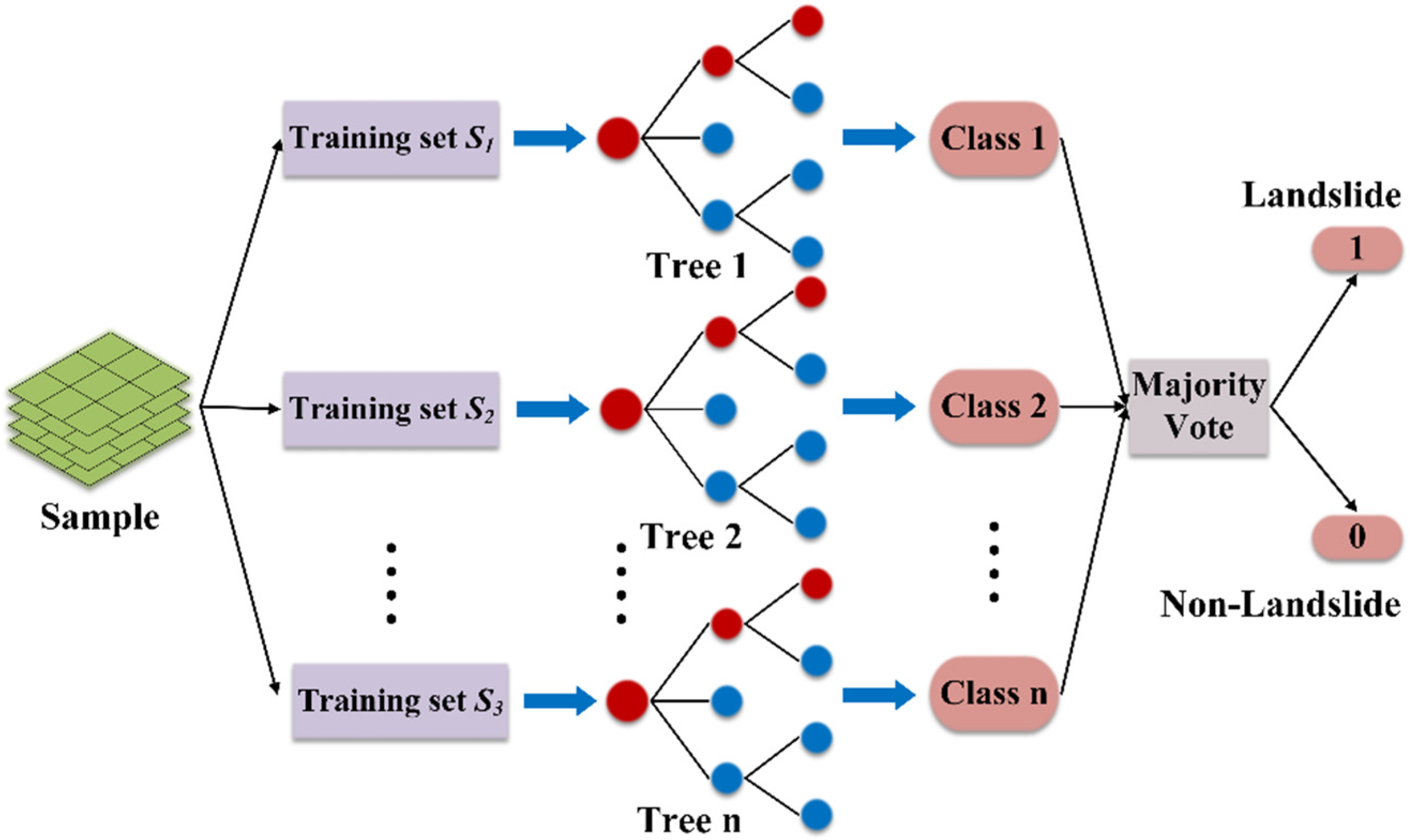
An RF model is a machine learning algorithm composed of multiple decision trees; it was proposed by Breiman based on the Bagging ensemble learning theory [54]. An RF model includes multiple decision trees trained by the Bagging ensemble learning algorithm. For a sample to be classified, the final result is determined via a voting mechanism of many decision trees; this method has solved the performance problem of decision trees, and it has good parallelism and expansibility for the classification of high-dimensional data and excellent tolerance for noise and abnormalities [55,56,57,58]. Unlike decision trees, the decision-making boundaries of an RF are several segmented functions (Figure 6). The Gini index was used in this study to analyze the importance of input factors in the RF algorithm.
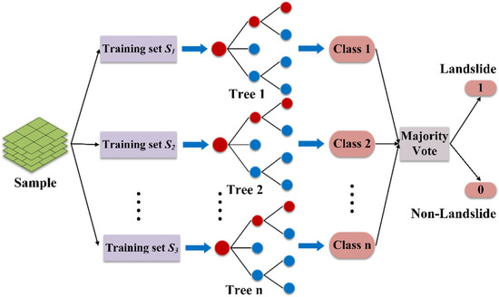
Figure 6.
Flow chart of the random forest model used in this study.
2.3.5. Accuracy Validation
In this study, the area under the ROC curve (AUC) and F1 were jointly used to measure the accuracy of the landslide prediction model [11,23,33]. The F1 is the harmonic mean of precision and recall, which is calculated as follows:
where TP (true positive) means that a positive sample was predicted to be positive, and FP (false positive) means that a negative sample was to be predicted positive.
An FN (false negative) result means that a positive sample was predicted to be negative, and a TN (true negative) result means that a negative sample was predicted to be negative. The greater the values of AUC and F1 are, the higher the accuracy of the model is.
3. Results
3.1. Factor Multicollinearity Analysis
If a correlation exists between the factors in landslide susceptibility mapping, the accuracy and efficiency of the model will be reduced. Therefore, it was necessary to analyze the correlation between the factors and remove any factors that were strongly correlated. Multicollinearity analysis was performed in SPSS software to obtain the values of tolerance (TOL) and variance inflation factors (VIFs) for correlation analysis. When TOL > 0.2, i.e., VIF < 5, the factors are independent of each other; thus, both factors can be used to build the regression model [59,60]. Table 1 shows that the VIFs of variables of all 12 disaster-inducing factors were less than 5, and the TOLs were greater than 0.2, indicating the independence between these factors. Hence, all 12 factors could be used in the model calculation.

Table 1.
Multicollinearity of Factors.
3.2. Selection of the Optimal Slope Unit
In the r.slopeunits method, the threshold (t) of the flow area (FA) and iterative coefficient (r) only control the numerical convergence of the data and have no geomorphological significance, whereas the minimum area (a) and circular variance (c) determine the size and direction of slope units. Because most landslides in the study area were medium-sized, the FA threshold was set to t = 1 × 10⁶ m2, the iterative coefficient r = 10, and cleansize = 2 × 10⁴ m2. The minimum area a was changed between a = 0.5 × 10⁵ m2, 1 × 10⁵ m2, 1.5 × 10⁵ m2, 2 × 10⁵ m2, 2.5 × 10⁵ m2 and 3 × 10⁵ m2, the circular variance c had a uniform distribution with an increment of 0.05 in the range of 0.1 ≤ c ≤ 0.4. A total of 42 groups of slope units at varying scales were obtained through different combinations of a and c. Figure 7 shows three slope units.

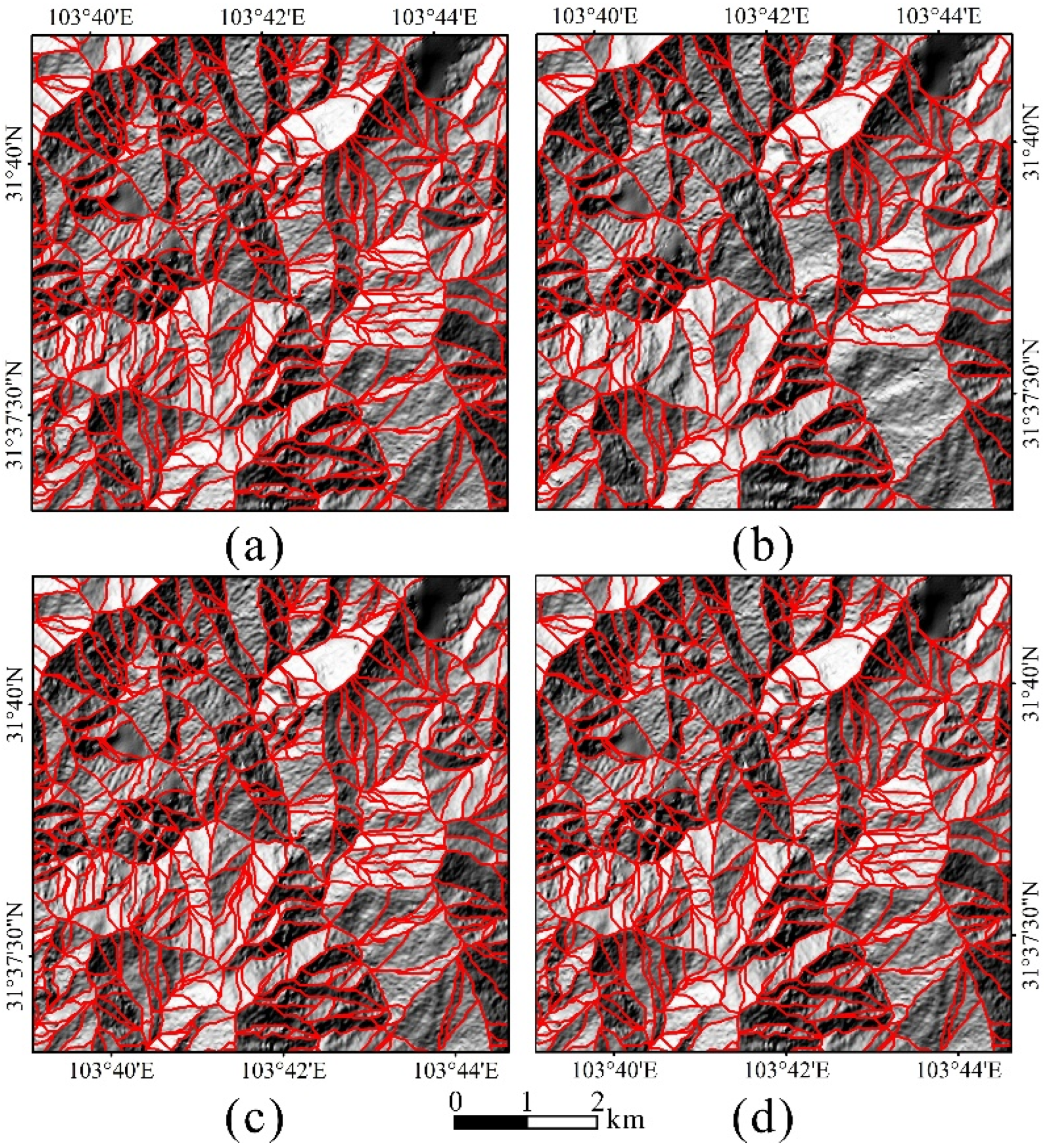
Figure 7.
Slope unit partition with different combinations of a and c in the same area: a is 1 × 10⁵ m2 in (a–d), and c is 0.1, 0.2, 0.15 and 0.3 in (a–d), respectively.
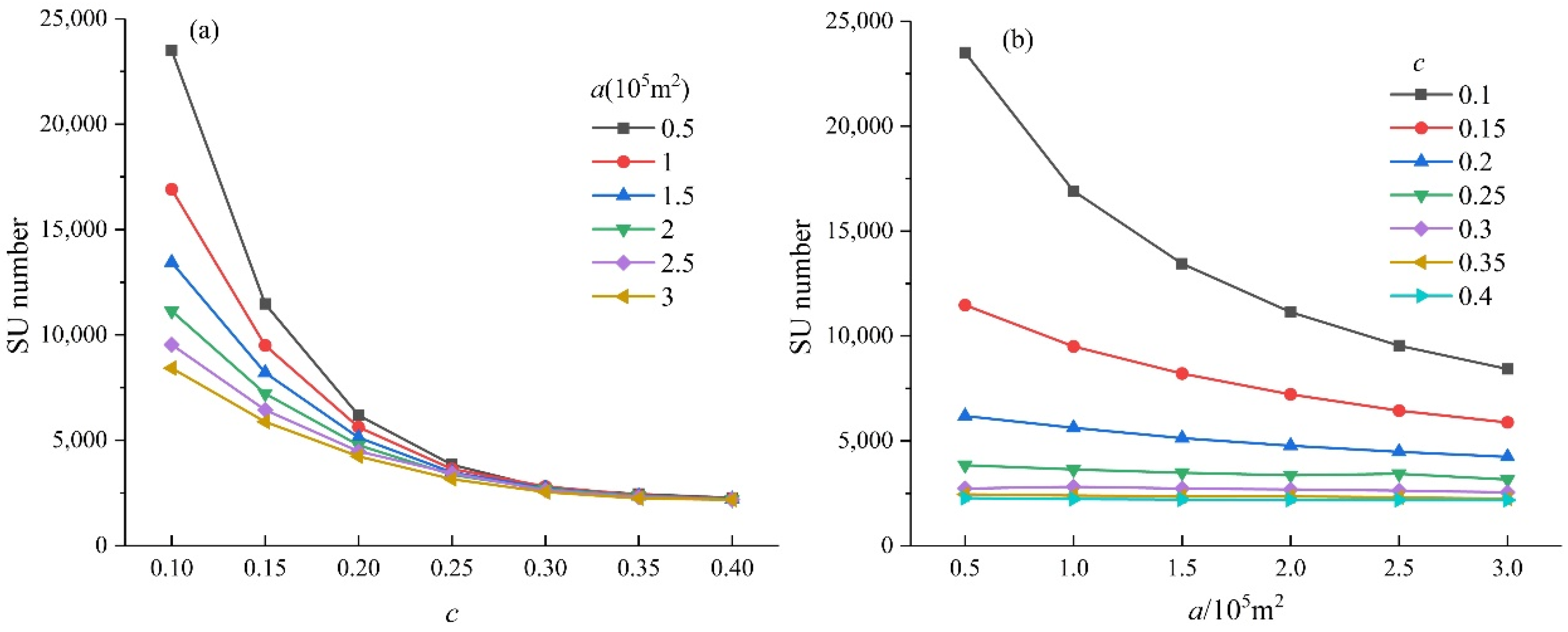
The number of slope units was used in this study to reflect different partition methods in the study area. Table 2 shows that the maximum partition number of slope units is 23,498 and the minimum number is 2242. Figure 8 shows the influence of different a and c combinations on the number of slope units. According to Figure 8a, when c ≥ 0.3, the number of slope units converges almost to the same value, suggesting that when c ≥ 0.3, the number of slope units does not change with c and a. From Figure 8b, (1) when c = 0.1, 0.15 or 0.2, the number of slope units changes as the value of a changes; the change is the smallest when c = 0.2, and the number of slope units starts to converge when a ≥ 1.5 × 10⁵ m2. (2) When a = 3 × 10⁵ m2, the number of slope units converges with different c values.
Table 2.
The number of Slope Units at Different Scales.
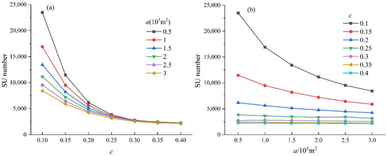
Figure 8.
The number of slope units with different (a) a and (b) c values.
Thus, the following 23 groups are of value in landslide susceptibility mapping in the study area, (1) c = 0.1, 0.15, and 0.2, combined with different a values, (2) c = 0.25 and a = 0.5 × 10⁵ m2, 1 × 10⁵ m2, 1.5 × 10⁵ m2 and (3) c = 0.3 and a = 0.5 × 10⁵ m2, 1 × 10⁵ m2.
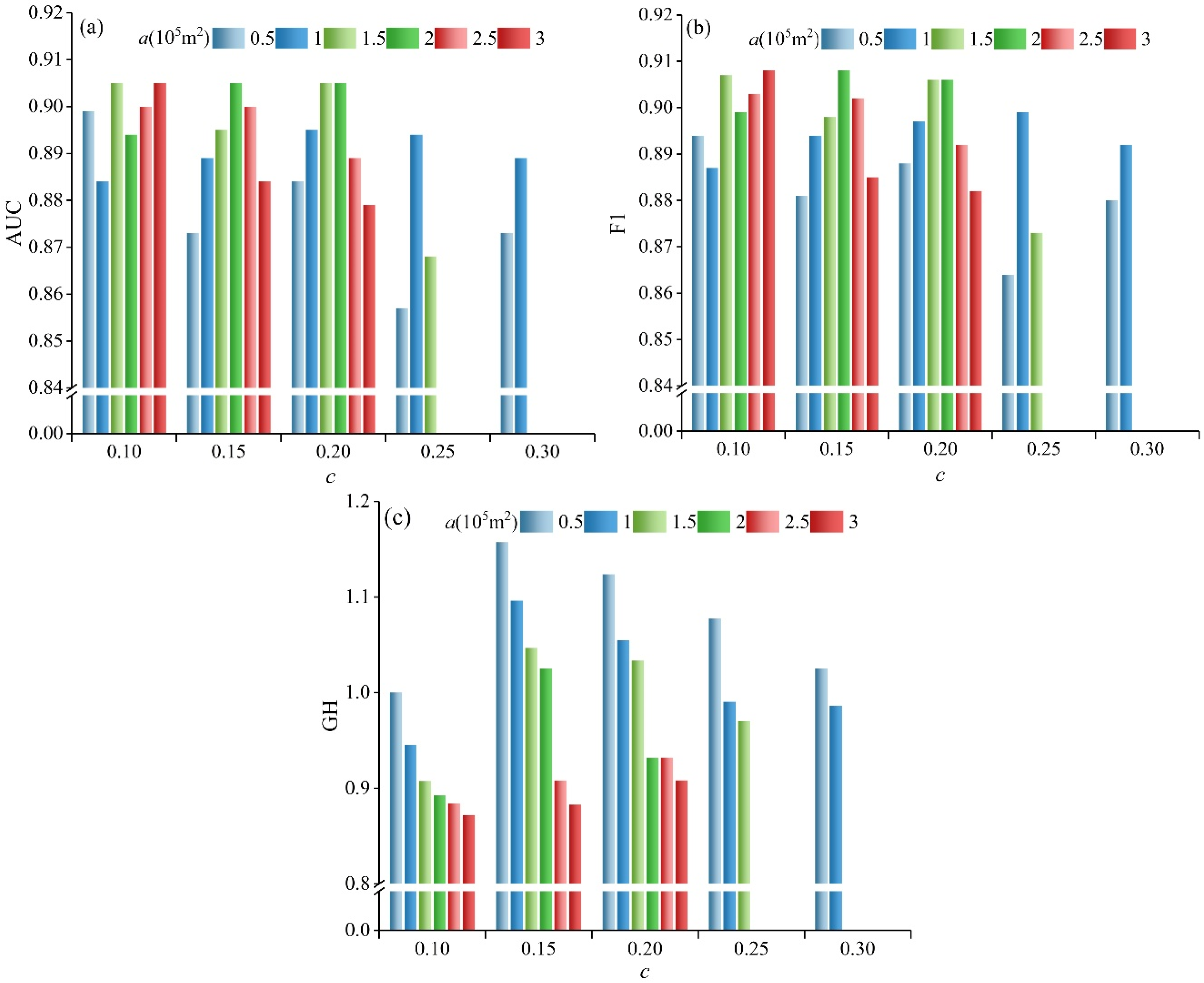
Susceptibility mapping was carried out for the 23 groups of slope units based on the IV-RF model, and the AUC and F1 values of the model were calculated (Figure 9a,b). Equation (6) was used to calculate the GH value of internal homogeneity and external heterogeneity of slope units (Figure 9c). In this paper, the maximum value of AUC was 0.905, and the minimum value was 0.857, with an average value of 0.890. Based on the conclusion of Hosmer and Lemeshow that AUC > 0.7 indicates high prediction accuracy, the proposed model in this study shows excellent spatial prediction ability.
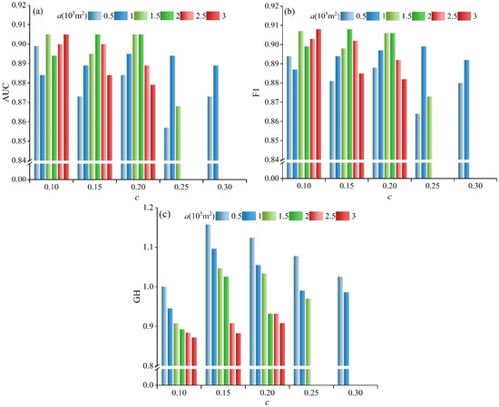
Figure 9.
AUC, F1 and GH values under different slope units: (a) AUC, (b) F1 and (c) GH.
Figure 9a,b show that there is little difference between AUC and F1, which had a similar trend. When c = 0.1, AUC and F1 reached the maximum values of 0.905 and 0.908 simultaneously at a = 3 × 10⁵ m2. When c = 0.15, AUC and F1 reach the maximum values of 0.905 and 0.908 simultaneously at a = 2 × 10⁵ m2. When c = 0.2, AUC and F1 reach the maximum values of 0.905 and 0.906 simultaneously at a = 1.5 × 10⁵ m2 and a = 2 × 10⁵ m2, respectively. When c = 0.25, AUC and F1 reach the maximum values of 0.894 and 0.899 simultaneously at a = 1 × 10⁵ m2. When c = 0.3, AUC and F1 reach the maximum values of 0.884 and 0.892 simultaneously at a = 1 × 10⁵ m2. Figure 9c shows that when c is a constant, the GH value decreases with the increase of a, indicating good partition results. The minimum value of GH was 0.872 when c = 0.1 and a = 3 × 10⁵ m2. In summary, the combination of c = 0.1 and a = 3 × 10⁵ m2 leads to the minimum GH and the maximum values of AUC and F1, i.e., optimal internal homogeneity and external heterogeneity and the best accuracy of landslide susceptibility mapping.
3.3. Landslide Susceptibility Map
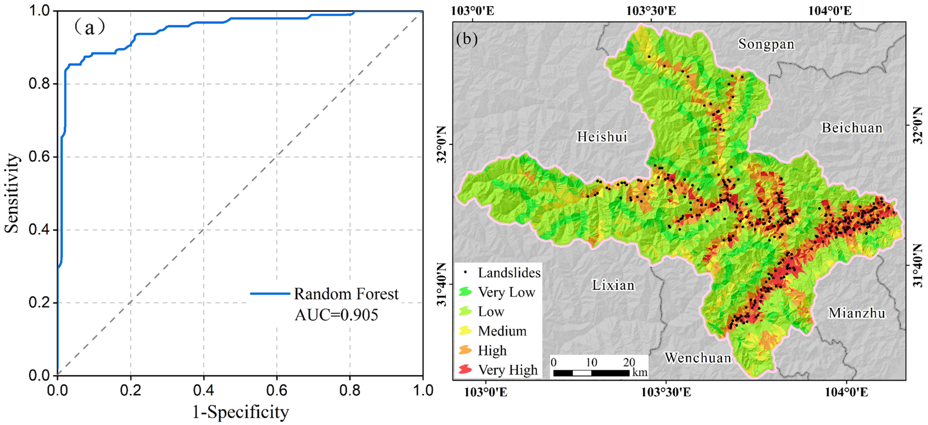
The landslide susceptibility indices of slope units extracted by the combination of c = 0.1 and a = 3 × 10⁵ m2 were divided into five grades: extremely high, high, medium, low and extremely low landslide susceptibility (Figure 10). Most areas of Maoxian County are located in the extremely low and low landslide susceptibility areas. Extremely high and high landslide susceptibility areas were mainly distributed in river valleys and both sides of major roads (e.g., Minjiang, Heishui and Tumen rivers, and road G213). The topography in these areas is fragmented and cracked, and the rocks are mostly phyllite and metamorphic rocks with an interbedded soft and hard rock structure, which can easily form a weak structural surface that is typically affected by rainfall and groundwater activities. The slope vegetation coverage in these areas was less than 10%; moreover, human economic activities and neotectonics are commonly present here. All these adverse factors contribute to the occurrence of landslides.
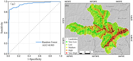
Figure 10.
(a) ROC curve; (b) Landslide susceptibility map.
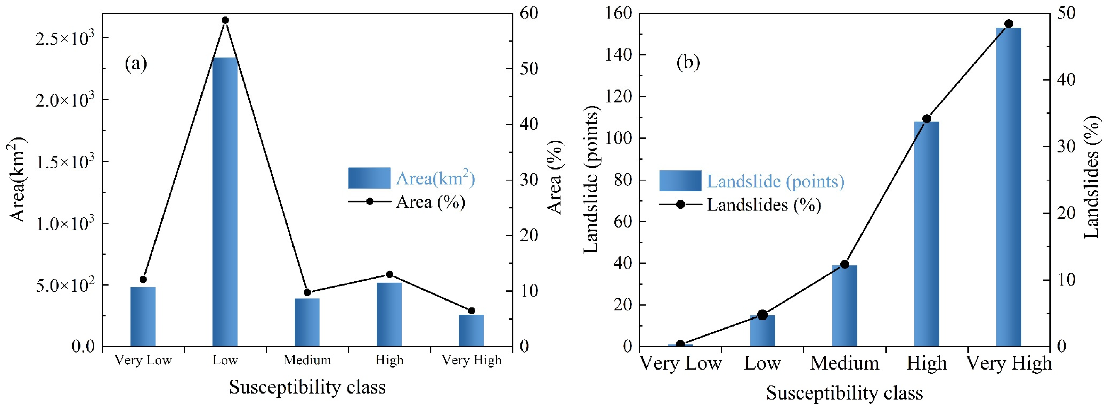
Table 3 and Figure 11 shows the number of slope units in each area with a different level of susceptibility and the number of previous landslides that occurred historically in each area. The proportion of previous landslides increased with an increase in the susceptibility grade. Areas of extremely low and low susceptibility accounted for 70.84% of the total area, and the number of previous landslides in these areas only accounted for 5.07% of the total number. In addition, areas of extremely high and high susceptibility only accounted for 19.41% of the total area, yet previous landslides here accounted for 82.60% of the total number. The results are in line with the actual situation.
Table 3.
Statistics of Different Susceptibility Areas.
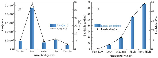
Figure 11.
Quantitative analysis of the susceptibility maps: (a) distribution of susceptibility classes; (b) frequency ratio of landslides in each susceptibility class.
4. Discussion
4.1. Reliability of the IV-RF Model
Multi-phase high-resolution remote sensing images, interferometric synthetic aperture radar (InSAR), historical landslide and field surveys were integrated to obtain 316 landslide samples with high accuracy; this study combines optical remote sensing with radar remote sensing to identify the potential landslide sites. Twelve factors were included, namely, seismic intensity, engineering strata, geological structure, slope gradient, slope aspect, curvature, TWI, RSP, distance from the nearest river, distance from the nearest road, mean annual precipitation and NDVI to carry out landslide susceptibility mapping based on the IV-RF. The IV model has been frequently used in previous studies [24,25]; however, it ignores the complex interactive relationship between the occurrence of landslides and factors influencing landslides. The RF model can capture the complex non-linear relationship between the factors and occurrence of landslides and has high prediction accuracy. In a study by Dou et al. [33], two groups of training samples were used to compare the landslide susceptibility mapping results of DT and RF models in the volcanic island area of Izu-Oshima in Japan [33]. The results showed that the RF model was superior to the DT model in different training sets; moreover, using logistic regression (LR), RF and support vector machine (SVM), Chang et al. [61] carried out landslide susceptibility mapping and found that RF has the best performance and is effective for DEMs with different resolutions. Numerous studies have shown that the mixed model has some advantages such as high accuracy and efficiency. Hence, the IV-RF model was adopted in this study to generate landslide susceptibility maps. In this study, the maximum value of AUC was 0.905, the minimum was 0.857, and the mean value was 0.890. According to Hosmer and Lemeshow, when AUC is greater than 0.7, the model has good prediction accuracy; thus, the proposed model in this study has excellent spatial prediction ability. The method based on slope unit scale and IV-RF model adopted in this study is suitable for landslide Susceptibility evaluation in areas with large topographic relief. In the future, we will strengthen the research on error conduction, numerical simulation of landslide and the correlation between landslide sensitivity evaluation results and landslide characteristics [62,63].
4.2. Optimal Mapping Units
The mapping unit is the basis of landslide susceptibility mapping. Different scales of mapping units will lead to different mapping results. Cama et al. [19] used forward stepwise binary logic regression (BLR) to model the susceptibility of an area to landslides with 2, 4, 16 and 32 m grid cells, the results of which showed that the 8 and 16 m groups have higher accuracy. The slope unit is the basic topographic unit of landslides, and currently few studies have analyzed the optimal slope unit scale in regional landslide susceptibility mapping. Positive and negative DEM hydrological analysis is the most common method used to extract slope units, yet this method is inefficient and is not conducive to the extraction of large-scale slope units, while the internal homogeneity of slope units is not considered. In comparison, the r.slopeunits method proposed by Alvioli et al. [17] can ensure the homogeneity of the slope aspect of the extracted slope units and controls the size and direction of slope units by the minimum area threshold a and circular variance c. The r.slopeunits method was used in this study to obtain 23 groups of slope units with different scales using different parameter combinations (a, c). The internal homogeneity of slope units and heterogeneity between different units were analyzed based on global aspect variance (V) and global weighted Moran index (wMI). The AUC and F1 were calculated to analyze the accuracy of the 23 groups of slope units in the IV-RF landslide susceptibility mapping model. Last, the optimal slope unit was decided based on V, wMI, ROC and F1. Specifically, when c = 0.1 and a = 3 × 10⁵ m2, the internal homogeneity and external heterogeneity of slope units were optimal, resulting in the best accuracy of landslide susceptibility mapping. The predicted spatial distribution of landslides in extremely high and high susceptibility areas was in line with the actual conditions.
The current study has some limitations. First, K-Means clustering was used to discretize continuous factors, so the clustering results may be ineffective if the initial clustering center in the K-Mean algorithm was not good. In the next step, we will compare the results of different clustering methods, such as hierarchical clustering, self-organizing-map (SOM) clustering, and Gaussian mixture model [64]. Second, non-landslide points in this study were random samples in areas about 1 km away from landslide points (buffer zone); however, there might be potential landslide points in the selected non-landslide points. Zhu et al. [65] has explored different methods such as a one-class support vector machine (one-class SVM), kernel density estimation, an artificial neural network (ANN) and a two-class support vector machine (two-class SVM) to generate non-landslide units. In a study by Huang et al. [66], a self-organizing-map (SOM) network was applied to generate the initial landslide susceptibility map and non-landslide grid cells were chosen from the extremely low susceptibility areas. A target spatial externalized sampling method was proposed by Xiao et al. [67] to generate non-landslide data directly using the eigenspace of existing landslides. We believe there will be more and more effective methods created that are designed to improve the quality of non-landslide points.
5. Conclusions
The objective of the present study was to carry out landslide susceptibility mapping in a deep valley area based on the optimal slope unit. The following conclusions are drawn.
(1) The mixed IV-RF model has excellent spatial prediction ability and accuracy in landslide susceptibility mapping.
(2) When c = 0.1 and a = 3 × 10⁵ m2, 8425 slope units were extracted by the r.slopeunits method, the internal homogeneity and external heterogeneity were optimal, indicating the model had the best level of accuracy. In other words, the optimal slope unit of a landslide susceptibility model is related to the category and size of landslides, rather than the size of slope units.
(3) The spatial distribution of high and extremely high susceptibility areas is consistent with that of existing landslides under the optimal slope units.
Author Contributions
Conceptualization, H.D., X.W. and W.L.; methodology, H.D., X.W., W.Z. (Wenjiang Zhang) and W.L.; software, X.W., X.L., Y.L. and W.Z. (Wenhao Zhuo); validation, P.Z.; analysis, X.W.; investigation, Y.L.; writing—original draft preparation, X.W. and H.D.; writing—review and editing, H.D. and W.L.; funding acquisition, H.D. and W.L. All authors have read and agreed to the published version of the manuscript.
Funding
This research was funded by the Key Research Program of Science and Technology Department of Tibet (XZ202001ZY0056G), Remote sensing identification and monitoring project of geologica hazards in Sichuan Province (510201202076888), Ministry of natural resources national geological hazard identification project in high risk areas (0733 20180876/2).
Data Availability Statement
The data presented in this study can be available on request from the corresponding author.
Acknowledgments
The authors would like to thank Qiang Xu, Ningsheng Chen and USGS for providing the research data, and also thank Dai and Li for patient guidance. The authors are also grateful to the editor and anonymous reviewers for their positive comments on the manuscript.
Conflicts of Interest
The authors declare no conflict of interest.
References
- Kirschbaum, D.; Stanley, T.; Zhou, Y. Spatial and temporal analysis of a global landslide catalog. Geomorphology 2015, 249, 4–15. [Google Scholar] [CrossRef]
- Lin, L.; Lin, Q.; Wang, Y. Landslide susceptibility mapping on a global scale using the method of logistic regression. Nat. Hazards Earth Syst. Sci. 2017, 17, 1411–1424. [Google Scholar] [CrossRef]
- Deng, Y.C.; Tsai, F.; Hwang, J.H. Landslide characteristics in the area of Xiaolin Village during Morakot typhoon. Arab. J. Geosci. 2016, 9, 332. [Google Scholar] [CrossRef]
- Fan, X.; Xu, Q.; Scaringi, G.; Dai, L.; Li, W.; Dong, X.; Zhu, X.; Pei, X.; Dai, K.; Havenith, H.-B. Failure mechanism and kinematics of the deadly June 24th 2017 Xinmo landslide, Maoxian, Sichuan, China. Landslides 2017, 14, 2129–2146. [Google Scholar] [CrossRef]
- Froude, M.J.; Petley, D.N. Global fatal landslide occurrence from 2004 to 2016. Nat. Hazards Earth Syst. Sci. 2018, 18, 2161–2181. [Google Scholar] [CrossRef]
- Smith, S.G.; Wegmann, K. Precipitation, landsliding, and erosion across the Olympic Mountains, Washington State, USA. Geomorphology 2018, 300, 141–150. [Google Scholar] [CrossRef]
- Ba, Q.; Chen, Y.; Deng, S.; Yang, J.; Li, H. A comparison of slope units and grid cells as mapping units for landslide susceptibility assessment. Earth Sci. Inform. 2018, 11, 373–388. [Google Scholar] [CrossRef]
- Zhao, S.; Zhao, Z. A Comparative Study of Landslide Susceptibility Mapping Using SVM and PSO-SVM Models Based on Grid and Slope Units. Math. Probl. Eng. 2021, 2021, 8854606. [Google Scholar] [CrossRef]
- Quesada-Román, A. Landslide risk index map at the municipal scale for Costa Rica. Int. J. Disaster Risk Reduct. 2021, 56, 102144. [Google Scholar] [CrossRef]
- Dou, J.; Yunus, A.P.; Bui, D.T.; Merghadi, A.; Sahana, M.; Zhu, Z.; Chen, C.-W.; Han, Z.; Pham, B.T. Improved landslide assessment using support vector machine with bagging, boosting, and stacking ensemble machine learning framework in a mountainous watershed, Japan. Landslides 2019, 17, 641–658. [Google Scholar] [CrossRef]
- Melchiorre, C.; Matteucci, M.; Azzoni, A.; Zanchi, A. Artificial neural networks and cluster analysis in landslide susceptibility zonation. Geomorphology 2008, 94, 379–400. [Google Scholar] [CrossRef]
- Yao, X.; Tham, L.G.; Dai, F.C. Landslide susceptibility mapping based on Support Vector Machine: A case study on natural slopes of Hong Kong, China. Geomorphology 2008, 101, 572–582. [Google Scholar] [CrossRef]
- Jia, N.; Mitani, Y.; Xie, M.; Tong, J.; Yang, Z. GIS deterministic model-based 3D large-scale artificial slope stability analysis along a highway using a new slope unit division method. Nat. Hazards 2014, 76, 873–890. [Google Scholar] [CrossRef]
- Wang, F.; Xu, P.; Wang, C.; Wang, N.; Jiang, N. Application of a GIS-Based Slope Unit Method for Landslide Susceptibility Mapping along the Longzi River, Southeastern Tibetan Plateau, China. ISPRS Int. J. Geo-Inf. 2017, 6, 172. [Google Scholar] [CrossRef]
- Wang, K.; Zhang, S.; DelgadoTéllez, R.; Wei, F. A new slope unit extraction method for regional landslide analysis based on morphological image analysis. Bull. Eng. Geol. Environ. 2018, 78, 4139–4151. [Google Scholar] [CrossRef]
- Penna, D.; Borga, M.; Aronica, G.T.; Brigandì, G.; Tarolli, P. The influence of grid resolution on the prediction of natural and road-related shallow landslides. Hydrol. Earth Syst. Sci. 2014, 18, 2127–2139. [Google Scholar] [CrossRef]
- Alvioli, M.; Marchesini, I.; Reichenbach, P.; Rossi, M.; Ardizzone, F.; Fiorucci, F.; Guzzetti, F. Automatic delineation of geomorphological slope units with r.slopeunits v1.0 and their optimization for landslide susceptibility modeling. Geosci. Model Dev. 2016, 9, 3975–3991. [Google Scholar] [CrossRef]
- Palamakumbure, D.; Flentje, P.; Stirling, D. Consideration of optimal pixel resolution in deriving landslide susceptibility zoning within the Sydney Basin, New South Wales, Australia. Comput. Geosci. 2015, 82, 13–22. [Google Scholar] [CrossRef]
- Cama, M.; Conoscenti, C.; Lombardo, L.; Rotigliano, E. Exploring relationships between grid cell size and accuracy for debris-flow susceptibility models: A test in the Giampilieri catchment (Sicily, Italy). Environ. Earth Sci. 2016, 75, 238. [Google Scholar] [CrossRef]
- Arabameri, A.; Pradhan, B.; Rezaei, K.; Lee, C.-W. Assessment of Landslide Susceptibility Using Statistical- and Artificial Intelligence-Based FR–RF Integrated Model and Multiresolution DEMs. Remote Sens. 2019, 11, 999. [Google Scholar] [CrossRef] [Green Version]
- Kayastha, P.; Dhital, M.; De Smedt, F. Application of the analytical hierarchy process (AHP) for landslide susceptibility mapping: A case study from the Tinau watershed, west Nepal. Comput. Geosci. 2013, 52, 398–408. [Google Scholar] [CrossRef]
- Pourghasemi, H.R.; Pradhan, B.; Gokceoglu, C. Application of fuzzy logic and analytical hierarchy process (AHP) to landslide susceptibility mapping at Haraz watershed, Iran. Nat. Hazards 2012, 63, 965–996. [Google Scholar] [CrossRef]
- Devkota, K.C.; Regmi, A.D.; Pourghasemi, H.R.; Yoshida, K.; Pradhan, B.; Ryu, I.C.; Dhital, M.R.; Althuwaynee, O.F. Landslide susceptibility mapping using certainty factor, index of entropy and logistic regression models in GIS and their comparison at Mugling–Narayanghat road section in Nepal Himalaya. Nat. Hazards 2012, 65, 135–165. [Google Scholar] [CrossRef]
- Sharma, L.P.; Patel, N.; Ghose, M.K.; Debnath, P. Development and application of Shannon’s entropy integrated information value model for landslide susceptibility assessment and zonation in Sikkim Himalayas in India. Nat. Hazards 2014, 75, 1555–1576. [Google Scholar] [CrossRef]
- Zhou, C.; Yin, K.; Cao, Y.; Ahmed, B.; Li, Y.; Catani, F.; Pourghasemi, H.R. Landslide susceptibility modeling applying machine learning methods: A case study from Longju in the Three Gorges Reservoir area, China. Comput. Geosci. 2018, 112, 23–37. [Google Scholar] [CrossRef]
- Regmi, N.R.; Giardino, J.R.; Vitek, J.D. Modeling susceptibility to landslides using the weight of evidence approach: Western Colorado, USA. Geomorphology 2010, 115, 172–187. [Google Scholar] [CrossRef]
- Goetz, J.N.; Brenning, A.; Petschko, H.; Leopold, P. Evaluating machine learning and statistical prediction techniques for landslide susceptibility modeling. Comput. Geosci. 2015, 81, 1–11. [Google Scholar] [CrossRef]
- Chen, W.; Ding, X.; Zhao, R.; Shi, S. Application of frequency ratio and weights of evidence models in landslide susceptibility mapping for the Shangzhou District of Shangluo City, China. Environ. Earth Sci. 2015, 75, 64. [Google Scholar] [CrossRef]
- Pradhan, B. A comparative study on the predictive ability of the decision tree, support vector machine and neuro-fuzzy models in landslide susceptibility mapping using GIS. Comput. Geosci. 2013, 51, 350–365. [Google Scholar] [CrossRef]
- Catani, F.; Lagomarsino, D.; Segoni, S.; Tofani, V. Landslide susceptibility estimation by random forests technique: Sensitivity and scaling issues. Nat. Hazards Earth Syst. Sci. 2013, 13, 2815–2831. [Google Scholar] [CrossRef] [Green Version]
- Chen, W.; Xie, X.; Wang, J.; Pradhan, B.; Hong, H.; Bui, D.T.; Duan, Z.; Ma, J. A comparative study of logistic model tree, random forest, and classification and regression tree models for spatial prediction of landslide susceptibility. Catena 2017, 151, 147–160. [Google Scholar] [CrossRef]
- Chen, W.; Xie, X.; Peng, J.; Shahabi, H.; Hong, H.; Bui, D.T.; Duan, Z.; Li, S.; Zhu, A.-X. GIS-based landslide susceptibility evaluation using a novel hybrid integration approach of bivariate statistical based random forest method. Catena 2018, 164, 135–149. [Google Scholar] [CrossRef]
- Dou, J.; Yunus, A.P.; Bui, D.T.; Merghadi, A.; Sahana, M.; Zhu, Z.; Chen, C.-W.; Khosravi, K.; Yang, Y.; Pham, B.T. Assessment of advanced random forest and decision tree algorithms for modeling rainfall-induced landslide susceptibility in the Izu-Oshima Volcanic Island, Japan. Sci. Total Environ. 2019, 662, 332–346. [Google Scholar] [CrossRef] [PubMed]
- Kanungo, D.; Arora, M.; Sarkar, S.; Gupta, R. A comparative study of conventional, ANN black box, fuzzy and combined neural and fuzzy weighting procedures for landslide susceptibility zonation in Darjeeling Himalayas. Eng. Geol. 2006, 85, 347–366. [Google Scholar] [CrossRef]
- Hong, H.; Pradhan, B.; Xu, C.; Bui, D.T. Spatial prediction of landslide hazard at the Yihuang area (China) using two-class kernel logistic regression, alternating decision tree and support vector machines. Catena 2015, 133, 266–281. [Google Scholar] [CrossRef]
- Mokarram, M.; Zarei, A.R. Landslide Susceptibility Mapping Using Fuzzy-AHP. Geotech. Geol. Eng. 2018, 36, 3931–3943. [Google Scholar] [CrossRef]
- Li, Y.; Chen, W. Landslide Susceptibility Evaluation Using Hybrid Integration of Evidential Belief Function and Machine Learning Techniques. Water 2019, 12, 113. [Google Scholar] [CrossRef]
- Merghadi, A.; Yunus, A.P.; Dou, J.; Whiteley, J.; ThaiPham, B.; Bui, D.T.; Avtar, R.; Abderrahmane, B. Machine learning methods for landslide susceptibility studies: A comparative overview of algorithm performance. Earth-Sci. Rev. 2020, 207, 103225. [Google Scholar] [CrossRef]
- Liu, W.; Cui, P.; Ge, Y.; Yi, Z. Paleosols identified by rock magnetic properties indicate dam-outburst events of the Min River, eastern Tibetan Plateau. Palaeogeogr. Palaeoclimatol. Palaeoecol. 2018, 508, 139–147. [Google Scholar] [CrossRef]
- Zhu, K.; Xu, P.; Cao, C.; Zheng, L.; Liu, Y.; Dong, X. Preliminary Identification of Geological Hazards from Songpinggou to Feihong in Mao County along the Minjiang River Using SBAS-InSAR Technique Integrated Multiple Spatial Analysis Methods. Sustainability 2021, 13, 1017. [Google Scholar] [CrossRef]
- Hakan, T.; Luigi, L. Completeness Index for Earthquake-Induced Landslide Inventories. Eng. Geol. 2020, 264, 105331. [Google Scholar] [CrossRef]
- Berardino, P.; Fornaro, G.; Lanari, R.; Sansosti, E. A new algorithm for surface deformation monitoring based on small baseline differential SAR interferograms. IEEE Trans. Geosci. Remote Sens. 2002, 40, 2375–2383. [Google Scholar] [CrossRef]
- Zhao, C.; Kang, Y.; Zhang, Q.; Lu, Z.; Li, B. Landslide Identification and Monitoring along the Jinsha River Catchment (Wudongde Reservoir Area), China, Using the InSAR Method. Remote Sens. 2018, 10, 993. [Google Scholar] [CrossRef]
- Costanzo, D.; Rotigliano, E.; Irigaray, C.; Jiménez-Perálvarez, J.D.; Chacón, J. Factors selection in landslide susceptibility modelling on large scale following the gis matrix method: Application to the river Beiro basin (Spain). Nat. Hazards Earth Syst. Sci. 2012, 12, 327–340. [Google Scholar] [CrossRef]
- Mattivi, P.; Franci, F.; Lambertini, A.; Bitelli, G. TWI computation: A comparison of different open source GISs. Open Geospat. Data Softw. Stand. 2019, 4, 6. [Google Scholar] [CrossRef]
- Fan, X.; Scaringi, G.; Xu, Q.; Zhan, W.; Dai, L.; Li, Y.; Pei, X.; Yang, Q.; Huang, R. Coseismic landslides triggered by the 8th August 2017 Ms 7.0 Jiuzhaigou earthquake (Sichuan, China): Factors controlling their spatial distribution and implications for the seismogenic blind fault identification. Landslides 2018, 15, 967–983. [Google Scholar] [CrossRef]
- Alvioli, M.; Guzzetti, F.; Rossi, M. Scaling properties of rainfall induced landslides predicted by a physically based model. Geomorphology 2014, 213, 38–47. [Google Scholar] [CrossRef]
- Capparelli, G.; Tiranti, D. Application of the MoniFLaIR early warning system for rainfall-induced landslides in Piedmont region (Italy). Landslides 2010, 7, 401–410. [Google Scholar] [CrossRef]
- Tsai, T.-L.; Yang, J.-C. Modeling of rainfall-triggered shallow landslide. Environ. Geol. 2006, 50, 525–534. [Google Scholar] [CrossRef]
- Gu, T.; Wang, J.; Fu, X.; Liu, Y. GIS and limit equilibrium in the assessment of regional slope stability and mapping of landslide susceptibility. Bull. Eng. Geol. Environ. 2014, 74, 1105–1115. [Google Scholar] [CrossRef]
- Espindola, G.M.; Camara, G.; Reis, I.A.; Bins, L.S.; Monteiro, A.M. Parameter selection for region-growing image segmentation algorithms using spatial autocorrelation. Int. J. Remote Sens. 2007, 27, 3035–3040. [Google Scholar] [CrossRef]
- Jain, A.K. Data clustering: 50 years beyond K-means. Pattern Recognit. Lett. 2010, 31, 651–666. [Google Scholar] [CrossRef]
- Xu, W.; Yu, W.; Jing, S.; Zhang, G.; Huang, J. Debris flow susceptibility assessment by GIS and information value model in a large-scale region, Sichuan Province (China). Nat. Hazards 2012, 65, 1379–1392. [Google Scholar] [CrossRef]
- Breiman, L. Random Forests. Mach. Learn. 2001, 45, 5–32. [Google Scholar] [CrossRef]
- Sahin, E.K.; Colkesen, I.; Kavzoglu, T. A comparative assessment of canonical correlation forest, random forest, rotation forest and logistic regression methods for landslide susceptibility mapping. Geocarto Int. 2020, 35, 341–363. [Google Scholar] [CrossRef]
- Guo, Q.; Zhang, J.; Guo, S.; Ye, Z.; Deng, H.; Hou, X.; Zhang, H. Urban Tree Classification Based on Object-Oriented Approach and Random Forest Algorithm Using Unmanned Aerial Vehicle (UAV) Multispectral Imagery. Remote Sens. 2022, 14, 3885. [Google Scholar] [CrossRef]
- Ye, Z.; Wei, J.; Lin, Y.; Guo, Q.; Zhang, J.; Zhang, H.; Deng, H.; Yang, K. Extraction of Olive Crown Based on UAV Visible Images and the U2-Net Deep Learning Model. Remote Sens. 2022, 14, 1523. [Google Scholar] [CrossRef]
- Ye, Z.; Guo, Q.; Zhang, J.; Zhang, H.; Deng, H. Extraction of urban impervious surface based on the visible images of UAV and OBIA-RF algorithm. Trans. Chin. Soc. Agric. Eng. (Trans. CSAE) 2022, 38, 225–234, (In Chinese with English abstract). [Google Scholar] [CrossRef]
- O’Brien, R.M. A Caution Regarding Rules of Thumb for Variance Inflation Factors. Qual. Quant. 2007, 41, 673–690. [Google Scholar] [CrossRef]
- Arabameri, A.; Saha, S.; Roy, J.; Chen, W.; Blaschke, T.; Bui, D.T. Landslide Susceptibility Evaluation and Management Using Different Machine Learning Methods in The Gallicash River Watershed, Iran. Remote Sens. 2020, 12, 475. [Google Scholar] [CrossRef] [Green Version]
- Chang, K.-T.; Merghadi, A.; Yunus, A.P.; Pham, B.T.; Dou, J. Evaluating scale effects of topographic variables in landslide susceptibility models using GIS-based machine learning techniques. Sci. Rep. 2019, 9, 12296. [Google Scholar] [CrossRef] [PubMed]
- Caviedes-Voullième, D.; Juez, C.; Murillo, J.; García-Navarro, P. 2D dry granular free-surface flow over complex topography with obstacles. Part I: Experimental study using a consumer-grade RGB-D sensor. Comput. Geosci. 2014, 73, 177–197. [Google Scholar] [CrossRef]
- Juez, C.; Caviedes-Voullième, D.; Murillo, J.; García-Navarro, P. 2D dry granular free-surface transient flow over complex topography with obstacles. Part II: Numerical predictions of fluid structures and benchmarking. Comput. Geosci. 2014, 73, 142–163. [Google Scholar] [CrossRef]
- Liang, Z.; Wang, C.; Duan, Z.; Liu, H.; Liu, X.; Ullah Jan Khan, K. A Hybrid Model Consisting of Supervised and Unsupervised Learning for Landslide Susceptibility Mapping. Remote Sens. 2021, 13, 1464. [Google Scholar] [CrossRef]
- Zhu, A.-X.; Miao, Y.; Yang, L.; Bai, S.; Liu, J.; Hong, H. Comparison of the presence-only method and presence-absence method in landslide susceptibility mapping. Catena 2018, 171, 222–233. [Google Scholar] [CrossRef]
- Huang, F.; Yin, K.; Huang, J.; Gui, L.; Wang, P. Landslide susceptibility mapping based on self-organizing-map network and extreme learning machine. Eng. Geol. 2017, 223, 11–22. [Google Scholar] [CrossRef]
- Xiao, C.C.; Tian, Y.; Shi, W.Z.; Guo, Q.H.; Wu, L. A new method of pseudo absence data generation in landslide susceptibility mapping with a case study of Shenzhen. Sci. China Technol. Sci. 2010, 53, 75–84. [Google Scholar] [CrossRef]


Publisher’s Note: MDPI stays neutral with regard to jurisdictional claims in published maps and institutional affiliations. |
© 2022 by the authors. Licensee MDPI, Basel, Switzerland. This article is an open access article distributed under the terms and conditions of the Creative Commons Attribution (CC BY) license (https://creativecommons.org/licenses/by/4.0/).