Global Empirical Models for Tropopause Height Determination

Abstract

The calculation of the tropopause height is crucial to the investigation of fundamental interactions between the troposphere and stratosphere, playing an essential role in areas such as climatology, geodesy, geophysics, ecology, and aeronautics. Since the troposphere and stratosphere have many distinct features, it is possible to define the boundary between them using different variables, such as temperature lapse rate, potential vorticity and chemical concentrations. However, according to the chosen variable, different tropopause definitions are created, each one with some limitations. Using 41 years of European Centre for Medium-Range Weather Forecasts (ECMWF) reanalysis (ERA5) data, we examined the variability of the tropopause for the north and south hemispheres and developed two models, both based on blending the potential vorticity and thermal tropopauses. One model (based on a sigmoid function, named STH) depends only on latitude and day of the year, while the other model (based on bilinear interpolation, named BTH) requires an additional look-up table. In order to account for the different behaviors of the tropopauses in the north and south hemispheres, we estimated two sets of model coefficients (one for each hemisphere). When compared against a benchmark of estimated tropopause heights during three years of radiosonde data, we obtained an average RMSE for the differences of 0.88 km for the STH model and 0.67 km for the BTH model. A similar comparison for alternative models available in the literature shows that the new models have superior performance and represent a significant improvement in tropopause height determination.

1. Introduction

The tropopause is the boundary between the upper troposphere and the lower stratosphere. These two atmospheric regions differ in numerous dynamical and chemical constituents. The troposphere is characterized by a negative temperature lapse rate between the top of the planetary boundary layer and the lower tropopause, with a mean value of 6.5 °C/km. This value varies due to interaction among radiative transfer, convection, and large-scale motions [1]. In contrast to the troposphere, the stratosphere is characterized by a temperature increase with height due to the Sun’s high-energy ultraviolet (UV) radiation absorption by the ozone (O₃) molecules present in this layer, converting the UV energy into heat. A close connection was observed between tropopause height (henceforth referred to as tropopause), tropospheric warming, and stratospheric ozone depletion (e.g., [2,3,4]). In fact, the tropopause can be located using ozonesonde profiles. However, these are sparse and rarely observed in the southern hemisphere (compared to the northern Hemisphere). The tropopause based on vertical ozone gradient is known as the chemical tropopause [5]. Other trace gases (or a combination) can be used, e.g., carbon monoxide (CO), which has higher concentrations in the troposphere, while ozone has higher concentrations in the stratosphere [6]. The ozone mixing ratio profile is also used in many tropopause studies (e.g., [3,7,8]). However, the threshold values can be challenging to determine.

In the last decade, some studies used a large dataset of bending angles (BAs) derived from the Global Navigation Satellite System Radio Occultation (GNSS-RO) to determine the tropopause. However, to derive physical atmospheric profiles, parametric dry atmospheric refractivity models are required [9,10,11]. In addition, the GNSS-RO vertical resolution is lower than the radiosondes resolution, which leads to lower accuracy.

The thermal tropopause is based on the knowledge of the temperature profiles [12], and can be determined using radiosondes, or a numerical weather model (NWM). However, its determination may present some complexity in the polar regions, showing a discontinuous surface with very high tropopauses in the vicinity of the polar jet [13], or discontinuities in the subtropical jet stream regions, where high tropical tropopause and a low extratropical tropopause are identified as one [14]. In addition to these limitations, the thermal definition cannot be used to characterize air masses, since the vertical temperature gradient is not a conservative quantity, even in the absence of an adiabatic process. Nevertheless, the thermal tropopause is used operationally and applied in several studies [15,16,17,18,19].

The dynamical tropopause is based on potential vorticity (PV) and is defined according to a given threshold value for PV [20]. It requires three-dimensional knowledge of meteorological quantities, e.g., wind and temperature, usually obtained from Numerical weather prediction (NWP) models. It has been suggested that the PV definition is more suitable for defining the tropopause, mainly in regions with strong cyclonic activity [17]. It also reveals advantages over the thermal definition since, in addition to considering the atmospheric stability, density and circulation are also taken into account. Furthermore, the PV surface is smoother than the thermal one due to its conservative properties under diabatic conditions. Usually, the dynamical tropopause is defined by the surface at which |PV| = 2 potential vorticity units (PVU; 1 PVU = 10⁻⁶ K kg⁻¹ m² s⁻¹). However, there is no consensus in the scientific community on the threshold value that defines tropopause. Several research studies have proposed a range of values between 1 and 5 PVU, depending on geographic location, seasonality, and atmospheric phenomena, e.g., [16,21,22,23,24,25,26]. The WMO [12,27] uses the 1.6 PVU value to define the dynamical tropopause. Hoerling et al. [28] applied the dynamical definition to the numerical weather model dataset from the European Centre for Medium-Range Weather Forecasts (ECMWF) and the thermal definition to radiosonde data. They suggested that the 3.5 PVU level represents an optimal value for the tropopause analysis outside the tropics, concluding that the 1.6 PVU, suggested by WMO [12], or values in a range of 1–3 PVU, proposed by other studies, substantially overestimate the tropopause. Zängl and Hoinka [17] compared both definitions. They concluded that the best agreement was found for a threshold value of 3.5 PVU. Therefore, the 1.6 PVU is not a suitable reference, especially for the polar regions in winter, when the 1.6 PVU surface drops below 700 hPa when subjected to strong cyclonic influences, making it possible that this surface can even intersect the ground. However, there is still no generally accepted value in the literature. Since potential vorticity values are positive in the northern hemisphere (NH) and negative in the southern hemisphere (SH), a dynamical approach in the tropical regions is not possible due to signal change, leading to very high and unrealistic PVU values. A variety of definitions and modern approaches to identifying the tropopause can be seen in Ivanova [29].

Even though there is an abundance of literature characterizing the tropopause, there is a lack of models that can be used to estimate the tropopause. In this study, we used 41 years’ worth of the European Centre for Medium-Range Weather Forecasts (ECMWF) Reanalysis 5th Generation (ERA5) [30] hourly data at model levels and 1° latitude–longitude horizontal resolution to develop two models for the tropopause. These models are based on the combination of the dynamical and thermal definitions to overcome the dynamical tropical region inversion and the discontinuous thermal surface in the polar zones. Furthermore, both models consider the geographic location and the day of the year. In addition, two sets of model coefficients were estimated for each hemisphere, accounting for different seasonal fluctuations. To broaden the applicability of these models, we also estimated coefficients for five PV surfaces, ranging from 1.6 to 3.5 PVU. Our goal was to develop a model based on primary inputs, such as geographic location and day of the year, that can be easily implemented and would be valuable in a wide range of applications, such as geodetic, climate studies, or even aviation, as aircraft fly close to the tropopause level [6,8,31,32]. Recently, climate change research has focused on the tropopause (e.g., [33,34,35,36,37]). Since our models are based on 41 years; worth of ERA5 data, they may be used as a reference in studies related to climate change, helping in the identification and monitoring of the tropopause fluctuations. An evaluation of the new tropopause models using a global radiosonde dataset is also included. This study is organized as follows: Section 2 describes the datasets used, the interannual variability verification, and the new model’s definition. In Section 3, we present the main results and discuss the models’ assessment, and, finally, conclusions are described in Section 4.

2. Datasets and Methods

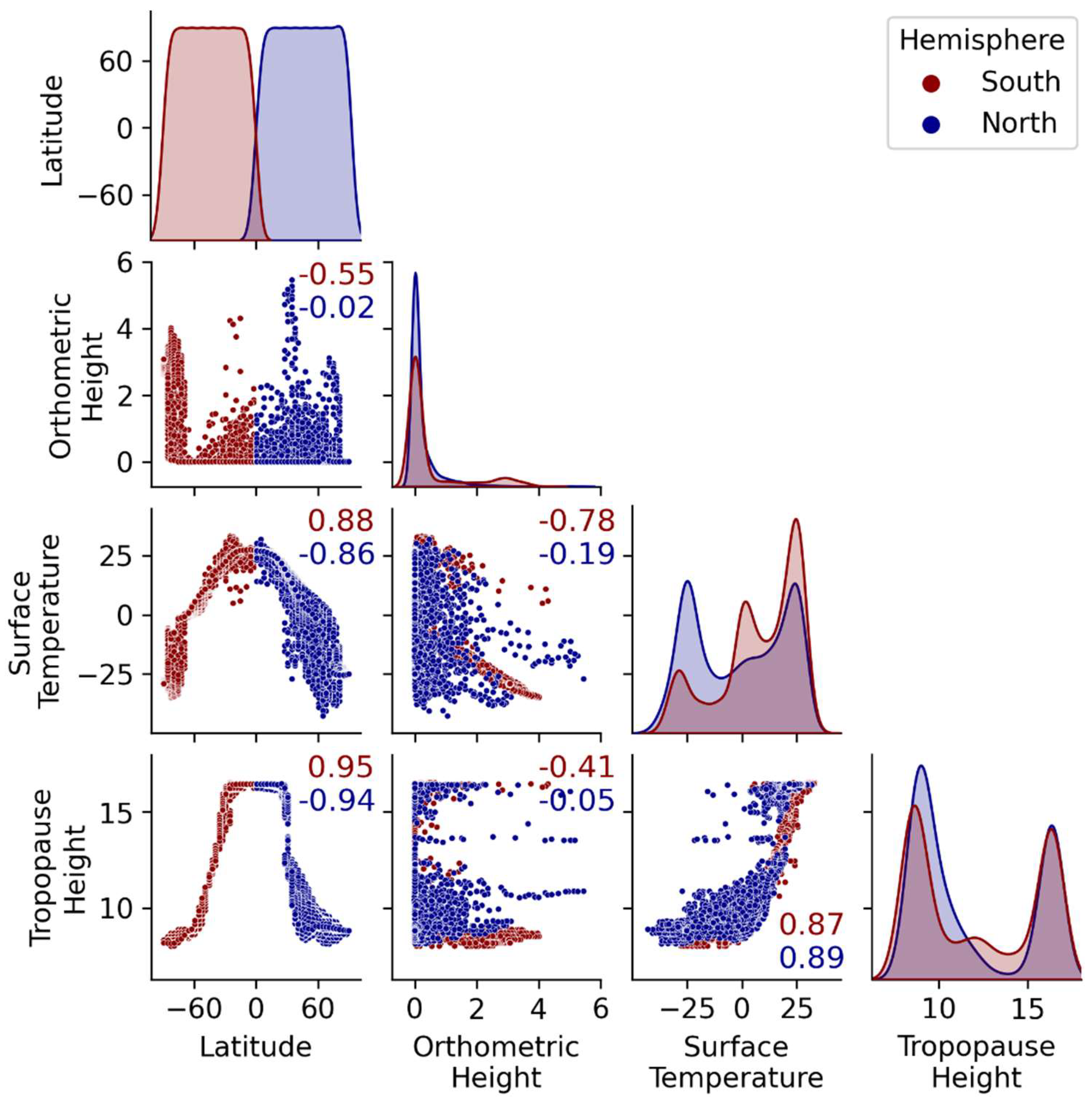
2.1. Weather Model Data

In order to develop new models for tropopause determination, we used the ERA5 model levels data [30]. The ERA5 model is the latest climate reanalysis produced by ECMWF, covering the period from 1950 onwards. It continues to be extended forward in time, being available 5 days behind real-time, with the quality-assured monthly data published within 3 months of real-time.

The ERA5 is the current state-of-the-art in numerical weather reanalysis field. When compared to its predecessor, the ERA-Interim model, the ERA5 provides significant innovations in core dynamics and model physics, uses a more advanced assimilation system, improves the horizontal resolution (from 79 km to about 30 km globally), has more vertical levels (from 60 to 137), and improves the temporal resolution (6 h to 1 h). Highlights of the significant improvements between ERA5 and ERA-Interim can be seen in Hersbach et al. [30,38]. However, the most significant ERA5 improvements are associated with the number of assimilated observations, which increased, on average, from 0.75 million per day, in 1979, to about 24 million per day, in 2018, boosted mainly by increased satellite observations and, more recently, by the GNSS-Radio Occultation, ozone measurements, and ground-based radar observations [38]. For this study, we used the ERA5 data at model levels (137 levels) from 1 January 1980 to 31 December 2020. This period was selected to avoid the inhomogeneities introduced in the transition to satellite data assimilation [39]. This product is available only in the ECMWF’s meteorological archive tapes (MARS), accessible through the Climate Data Store (CDS) Application Programming Interface (API).

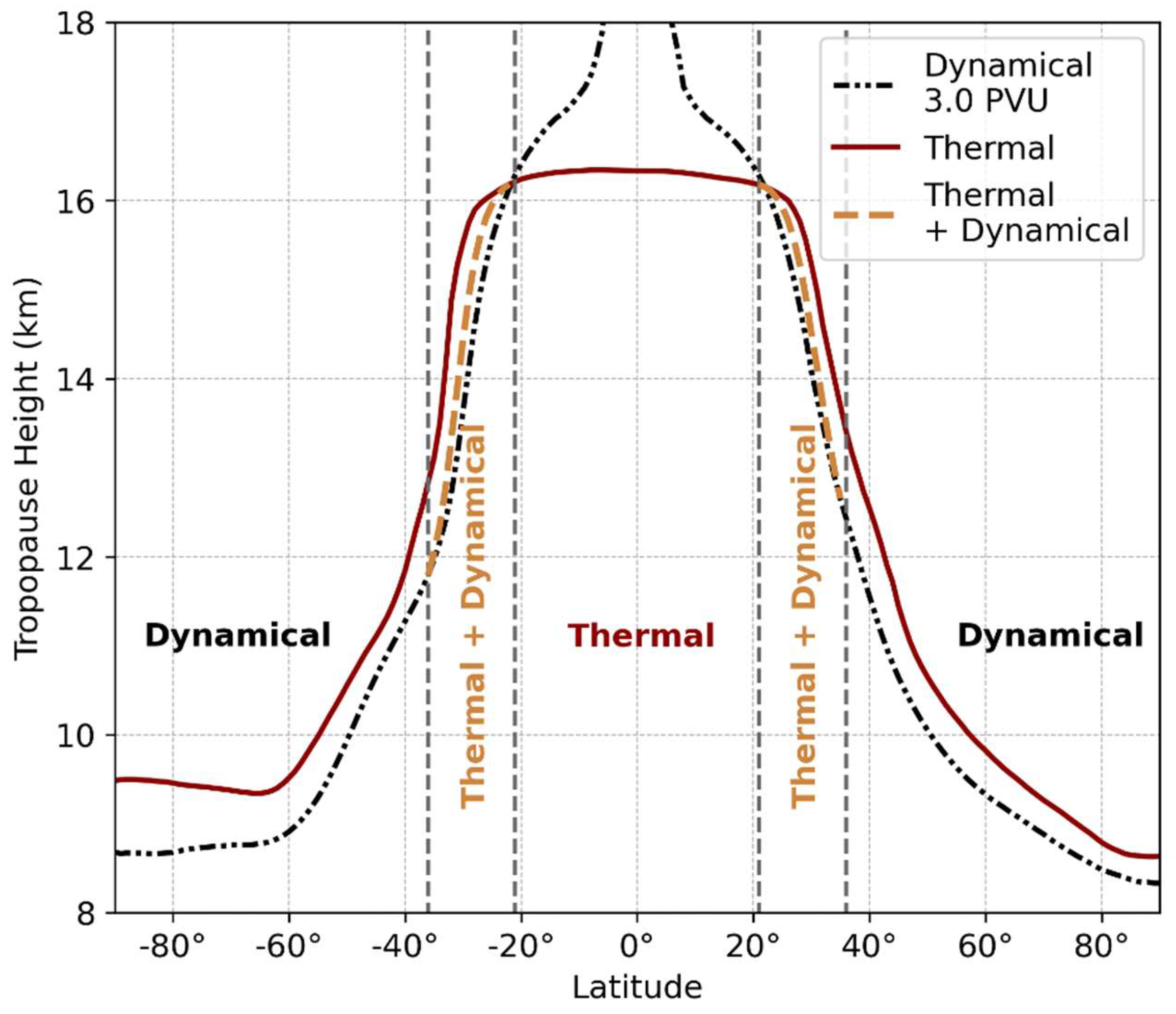
2.2. Dynamical Tropopause

The dynamical tropopause concept was introduced by Reed [21] and is based on potential vorticity (PV). It can be expressed as [40]:

$$PV=-g\left({\zeta }_{\theta }+f\right)\frac{\partial \theta }{\partial p},{\zeta }_{\theta }={\left(\frac{\partial v}{\partial x}-\frac{\partial u}{\partial y}\right)}_{\theta }$$

(1)

where $g$ is the acceleration due to gravity (m s⁻²), ${\zeta }_{\theta }$ is the relative vorticity calculated on the isentropic surface (s⁻¹), $f$ is the Coriolis parameter (latitude dependent) (rad s⁻¹), θ is the potential temperature (K), $p$ is the pressure (Pa), $u$ is the zonal wind component (m s⁻¹), $v$ the meridional wind component (m s⁻¹), and PV is the potential vorticity (K m² kg⁻¹ s⁻¹). The PV quantity is not available in the ERA5 model-level dataset. In order to calculate the PV in all model levels, we used the zonal and meridional wind components, the temperature, the geopotential, and the specific humidity provided by ERA5. The last two parameters are needed to convert from model to pressure levels.

A less time-consuming alternative is to use monthly mean PV data available at monthly pressure levels. However, PV is a non-linear quantity. Therefore, we computed the PV at the model level for each day and averaged it into monthly means. Note that the monthly PV quantities (available at monthly pressure levels) result in a smooth field that may compare patterns well but is likely to lack the detailed structure of monthly mean PV. In addition, the pressure model levels have a coarse vertical resolution compared with the model level dataset. Since this task is computationally expensive, the temporal resolution was limited to 6 h, the horizontal grid was spatially interpolated to 1°, and all levels above 30 km altitude were excluded.

We used the NCL (NCAR Command Language) package that implements Equation (1) to compute PV at model levels. The script uses highly accurate spherical harmonic functions to compute horizontal gradients over a global grid. It also outputs static stability and potential temperature. The algorithm details can be seen in Buja [41]. Note also that PV values at SH were negative. In the methods described below, we use the PV module. The geopotential height was calculated by the ratio between the geopotential and the gravitational acceleration. The gravitational acceleration varies with latitude and height and can be calculated using Equation (2) [42]:

$$g=9.780327\times \left[1+0.00530024\sin {\left(\phi \right)}^2-0.0000058\sin {\left(2\phi \right)}^2\right]-3.086\times {10}^{-6}H$$

(2)

where $H$ is the orthometric height (m), and $\phi$ is the latitude (rad), both obtained from ERA5 single-level dataset.

We computed monthly averages of geopotential height and PV, resulting in 492 datasets, and we selected five surface heights corresponding to 1.6, 2.0, 2.5, 3.0, and 3.5 PVU values. To find the surface height with PV close to a PVU value, we proceeded as follows: (1) the selected PVU value level was located for each vertical grid profile. Possible low-level strong potential vorticity values close to the surface were suppressed by considering only the levels above 550 hPa (at ≈5 km). This way, the influence of thermal inversion was removed from the data, avoiding the detection of false tropopauses close to the surface; (2) assuming that PVU varied linearly in that level (1), the lowest and highest pairs of height and PV values, ($z_i,{\mathrm{PV}}_i$) and ($z_{i+1},{\mathrm{PV}}_{i+1}$), were used to obtain the height where PVU was equal to one of the five selected values by linear interpolation.

Due to the PV sign change near the equator, the dynamical tropopause approach applies only in extra-tropics. Therefore, the thermal definition is the only criterion that can be applied in the tropics.

2.3. Thermal Tropopause

The thermal tropopause is based on the principle that the stratosphere has a more stable stratification than the troposphere. This suggests that the stratospheric lapse rate is smaller than the tropospheric lapse rate (a), defined as the rate of change of temperature with height:

$$\mathsf{\alpha }=-\frac{dT}{dz}$$

(3)

where dT is a change in temperature in a layer thickness of dz; the signal is conventionally chosen so that the lapse rate is considered positive when the temperature decreases with height, is negative when the temperature increases with height (thermal inversion), and zero when the temperature is constant with height. This study adopted the WMO [12] thermal tropopause definition: “the lowest level at which the lapse rate decreases to 2 °C/km or less, provided also that the average lapse rate between this level and all higher levels within 2 km does not exceed 2 °C/km”. Therefore, we calculated the lapse rate using the temperature and geopotential height from the ERA5 model-levels dataset. Each lapse rate was assigned to the middle of the corresponding layer. In order to avoid thermal inversion, only levels above 550 hPa (at ≈5 km) were considered, similar to the strategy used in the dynamical tropopause. For each lapse rate vertical profile, the first level, from below, not exceeding 2 °C/km was fixed, and the average lapse rate in the following 2 km was calculated. If the average value was smaller, or equal to, 2 °C/km, then the first level fixed fulfilled both parts of the lapse rate criterion. If the second criterion was not fulfilled, we searched for the next level where the lapse rate was below 2 °C/km. The exact value of the tropopause was linearly interpolated using the lowest ($z_i,{\mathsf{\alpha }}_i$) and highest ($z_{i+1},{\mathsf{\alpha }}_{i+1}$) height and lapse rate values of the fixed level. According to the WMO [12], if the average lapse rate between any level above the first tropopause and any level inside the next higher kilometer is less than 3 °C/km, an additional tropopause can be found using the same criteria as before. Multiple tropopauses are most common in the sub-tropical regions, where large horizontal temperature contrast can be found. In this case, the tropopause is computed directly from the temperature profile by locating the local minimum [10].

2.4. Dynamical and Thermal Tropopause Blend

To overcome the dynamical tropopause limitation across the equatorial region, our models were based on a blend of both tropopauses. The thermal tropopause was used as a threshold value for the dynamical tropopause between the subtropical and the tropical latitudes, ensuring continuity and smoothness between both tropopauses. This approach had two main steps: (1) we determined the latitude at which the dynamical tropopause surpassed the thermal tropopause (for both hemispheres). At these latitudes, the thermal tropopause values replace the dynamical tropopause values; (2) a weighted average of both tropopauses was applied in a latitude band with 15° to ensure smoothness. In the 15° band, the weighted function decreased linearly with the increased distance to the equator. Figure 1 shows an example of the approach described, considering the 3.0 PVU surface height.

Table 1. Latitude bands (in absolute values) to combine thermal and dynamical tropopauses. The middle band (Dynamical + Thermal) is used to ensure continuity and smoothness.

Type	PVU Value/Latitude
	1.6	2.0	2.5	3.0	3.5
Dynamical	90°–25°	90°–29°	90°–33°	90°–36°	90°–39°
Dynamical + Thermal	25°–10°	29°–14°	33°–18°	36°–21°	39°–24°
Thermal	10°–0°	14°–0°	18°–0°	21°–0°	24°–0°

shows the zonal bands used for each PVU surface.

As an example, Figure 2 represents the combined mean tropopause for each month for the case of the 3.5 PVU surface. As expected, the highest tropopauses could be observed in the tropics zone, with a maximum value reaching about 17.5 km over the southwest of Asia during the NH summer. The lowest tropopause of about 7.5 km could be observed over the polar zones. The north polar zone showed a mean tropopause oscillation between 7.8 km (NH winter months) and 8.9 km (NH summer months), corresponding to a mean tropopause temperature variation of 14 °C (from −57 °C to −43 °C). The south polar zone showed the lowest mean height of about 7.5 km during the SH summer, reaching about 9.2 km during the SH winter months, corresponding to a mean tropopause temperature variation of 17 °C (from −50 °C to −67 °C). When comparing polar zones, the greatest mean tropopause difference (~700 m) can be observed during the NH summer months, when the temperature difference between hemispheres is significant (~24 °C). The reverse behavior is not observed in the SH summer months, since the temperature of the summer Antarctic is close to the temperature of the winter Arctic [17]. Significant spatial variations of tropopause appeared above the sub-tropical zones. For example, in the NH subtropical zone (between 23° and 35°), the tropopause dropped about 4.5 km (in all months). However, the same decrease in the summer months was only observed between 23° and 43°. Similar behavior was seen in the southern subtropical zone.

Since the NH seasonal cycle reveals different characteristics compared to the SH seasonal cycle, mainly during the summer NH months, an analysis of the annual cycle spatial patterns can be helpful to distinct spatial trends between both hemispheres. So, we computed the mean tropopause anomalies for each month (using the 3.5 PVU surface as reference). Figure 3 shows the tropopause anomaly zonal profiles for each month. In the winter NH months, negative anomalies (lower tropopauses) were present in the subtropics zone, showing a well-defined longitudinal band, close to the location of the subtropical jet streams, in the transition between the Hadley and Ferrel cells, that could also be observed in the SH with positive anomalies (higher tropopauses). Nevertheless, a positive anomaly band could be observed in the NH summer months, moving some degrees of latitude, mainly over land, toward the pole. The meridional and seasonal variations in the mean zonal tropopause (and tropopause temperature) were characterized by a minimum and maximum during the NH winter and summer months, respectively, associated with the global jet stream structure. Furthermore, the tropopause pattern variability was positively correlated with the corresponding tropospheric temperature patterns (not shown). Other studies showed similar results, e.g., [10,17,43,44,45].

As expected, both hemispheres displayed two distinct behaviors (see Figure 3) that varied with the season, atmospheric circulation, and even with the unequal distribution of land between hemispheres, which influenced the weather [46].

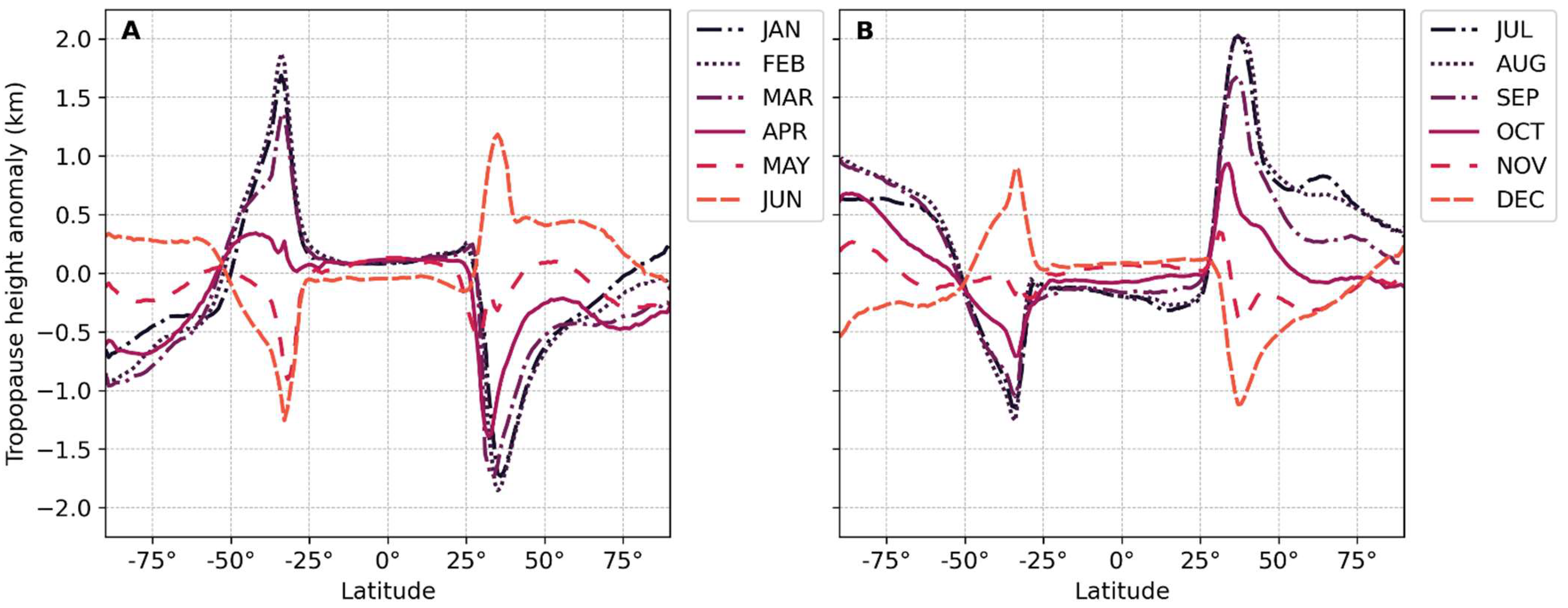
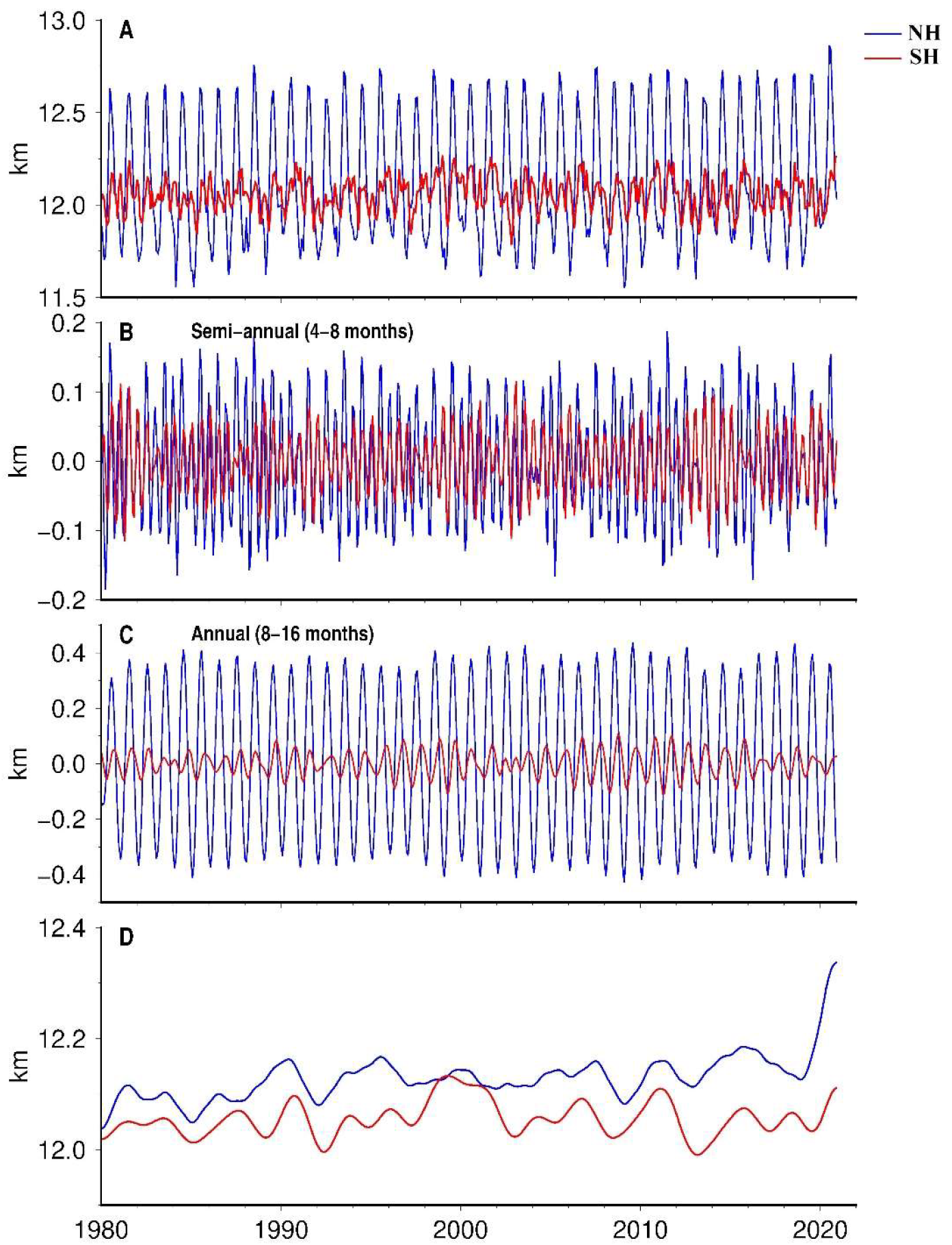
2.5. Tropopause Variability

We used a discrete wavelet transform (DWT) to decompose each time series into different scales with corresponding frequency bands and a trend signal to analyze the variability of the average hemispheric tropopause on both hemispheres. Figure 4 shows the original time series (top), the levels corresponding to the semi-annual (B) and annual variations (C), and the trend signals (D). Panel A displays the mean monthly tropospheric variation using the 3.5 PVU surface (NH identified by a blue line and SH by a red line), with an NH mean value of 12.13 km and 12.06 km for the SH. The mean global value was 12.10 km. This value agreed with the one proposed by Lanyi [31] of 12.2 km and was very close to the one proposed by Mendes [47] of 11.9 km. The NH showed a peak-to-peak variation of 1.3 km and the SH of 0.5 km. The semi-annual and annual SH signals had a similar contribution explaining more than 70% of the total variation (panel A, red line). In the case of NH, the annual signal contributed significantly more (about 90%) to the total signal (panel A, blue line) than the semi-annual contribution (about 9%).

Panel D shows the main trend for both hemispheres. The NH tropopause revealed a mean linear trend of 21.9 ± 1.2 m decade⁻¹, mainly stimulated by increased tropopause temperature in the hot NH months (June to October). The SH tropopause also revealed a positive linear trend of about 3.2 ± 1.2 m decade⁻¹. Nevertheless, the most significant velocities were found during the winter SH months (June to October). Both curves (blue and red) showed a high Pearson correlation coefficient of 0.9. The mean difference between the trend verified for both hemispheres was about 150 m but increased about 12 m decade⁻¹. We applied a two-tailed t-test [48] to test whether the trends for both hemispheres (β₁ and β₂) were equal, i.e., we stated the null hypothesis H₀: β₁ = β₂ and the alternative hypothesis H₁: β₁ ≠ β₂. We obtained a p-value of 6.53 × 10⁻¹⁵⁷, so we rejected the null hypothesis of no difference between trends at a 5% significance level. These results corroborated other studies that attributed the positive trend to not only a dominant anthropogenic process but also to other natural external forcings [4,18,45,49,50].

2.6. Numerical Models

The DWT results show that a model for each hemisphere, taking into account a seasonality component, should be considered to achieve the best accuracy for determining tropopause. Apart from this, we also analyzed the correlation between tropopause and other parameters, such as latitude, orthometric height, and surface temperature. Figure 5 shows the correlation matrix that describes the correlation between the mentioned parameters. The numbers in each subplot show the Pearson correlation coefficient ($\rho$) by hemisphere. As an example, Figure 5 shows the lower triangular matrix of correlations for January (for clarity, only 91 × 180 grid points were considered). It is clear that the tropopause was better described as a function of the latitude, with very strong correlation values in all months ($\rho$ ≥ 0.90). The tropopause also correlated with the day of the year, as is evident in Figure 4. A visual inspection of the relationship between the tropopause and latitude suggested that a sigmoid function could be used as an adequate model. The tropopause also revealed a strong correlation ($\rho$ ≥ 0.70) with surface temperature, coming essentially from the latitudinal effect. However, the plot shape suggested that an exponential type of function was more suitable for describing the tropopause dependence with surface temperature. Since our goal was to develop a model that depends on the minimum number of input parameters (latitude and day of the year), we used a five-parameter sigmoid function with a second term to model the seasonality.

The adopted tropopause model (named STH) is given by:

$$f\left(\phi ,doy\right)=a_0+\frac{a_1}{{\left(1+\exp \left(-\frac{\phi -a_2}{a_3}\right)\right)}^{a_4}}+a_5·cos\left(\frac{2\pi \left(doy-28\right)}{365.25}\right)$$

(4)

where the first two-term is the sigmoid function, depending only on the latitude ($\phi$, in degrees), and the last term is the seasonal term depending on the day of the year ($doy$, UTC days since the beginning of the year). The $a_{0-4}$ are the five sigmoid coefficients, and $a_5$ is the seasonal coefficient. We adopted the value of the phase of 28 days obtained by Niell [51] and also adopted by others (e.g., Mendes et al. [52]). The coefficients were estimated for each tropopause (1.6, 2.0, 2.5, 3.0, and 3.5 PVUs) using a Levenberg-Marquardt non-linear iterative least-squares algorithm [53] in the training period from 1980 to 2017. We chose not to include the PVU value as an additional input parameter in the model because adding another term would increase its complexity and not necessarily its accuracy. The different coefficients for each PVU model are listed in

Table 2. Coefficients ($a_{0-5}$) estimated for Southern Hemisphere, see Equation (4).

PVU VALUE	$a_0$	$a_1$	$a_2$	$a_3$	$a_4$	$a_5$
1.6	7.209 (±0.040)	9.119 (±0.040)	−18.95 (±0.24)	1.81 (±0.23)	0.107 (±0.015)	−0.18593 (±0.00075)
2.0	7.775 (±0.037)	8.552 (±0.037)	−21.36 (±0.21)	1.36 (±0.24)	0.088 (±0.016)	−0.16402 (±0.00064)
2.5	8.180 (±0.036)	8.146 (±0.036)	−23.48 (±0.21)	1.15 (±0.25)	0.079 (±0.018)	−0.14909 (±0.00063)
3.0	8.505 (±0.036)	7.818 (±0.036)	−25.32 (±0.22)	1.11 (±0.25)	0.082 (±0.019)	−0.13704 (±0.00071)
3.5	8.779 (±0.039)	7.542 (±0.039)	−26.73 (±0.24)	1.15 (±0.25)	0.087 (±0.021)	−0.1255 (±0.0010)

and

Table 3. Coefficients ($a_{0-5}$ ) estimated for Northern Hemisphere, see Equation (4).

PVU VALUE	$a_0$	$a_1$	$a_2$	$a_3$	$a_4$	$a_5$
1.6	7.145 (±0.066)	9.185 (±0.067)	20.12 (±0.43)	−2.81 (±0.33)	0.151 (±0.022)	−0.186 (±0.018)
2.0	7.650 (±0.060)	8.677 (±0.062)	22.43 (±0.38)	−2.32 (±0.32)	0.133 (±0.022)	−0.164 (±0.017)
2.5	7.993 (±0.056)	8.333 (±0.058)	24.17 (±0.33)	−1.81 (±0.32)	0.108 (±0.021)	−0.149 (±0.016)
3.0	8.265 (±0.055)	8.058 (±0.057)	25.56 (±0.31)	−1.55 (±0.32)	0.095 (±0.022)	−0.137 (±0.016)
3.5	8.499 (±0.057)	7.823 (±0.058)	26.73 (±0.33)	−1.58 (±0.34)	0.098 (±0.023)	−0.126 (±0.016)

for the southern and northern hemispheres. Figure 6 (left panel) depicts the tropopause computed for both hemispheres using the STH model with the 3.5 PVU coefficients.

An alternative lookup-table model (named BTH) is based on two variables grid bilinear interpolation followed by linear interpolation for the requested PVU value. Compared to the model introduced above, the disadvantage is that knowledge of the model coefficients is needed (computer code that implements this model is available at https://github.com/pjmateus/global_tropopause_model, accessed on 1 July 2022). This model was established according to the following steps. Firstly, we obtained, zonal tropopause profiles for each PVU surface and month (5 × 12 × 181). Secondly, the latitude was interpolated to a non-evenly spaced grid, i.e., from 90° to 45° and 10° to 0° (SH and NH), a mean tropopause value every 10° latitude was calculated, and between 45° and 10° a value every 5° latitude (5 × 12 × 23), see Figure 6 (right panel). In addition, the 5° latitude interval was implemented to improve the model’s accuracy in the sub-tropical region (high-pressure zone in the transition between the Hadley and Ferrel cells). Finally, using bilinear interpolation, the tropopause was calculated for a given pair of latitude and doy (for each of the 5 PVU values), followed by linear interpolation to obtain the correct tropopause at the requested PVU value. One advantage of this model is that the tropopause can be calculated for any PVU value. However, results for PVUs below 1.6 and above 3.5 were extrapolations and must be used with caution.

Table 4. Mean Root-mean-square error (RMSE) and bias values of the STH and BTH model fit, respectively, for each PVU value and hemispheres (in m). Values in parentheses identify the bias. A positive bias indicates a model overestimation.

Model	Hemisphere	PVU Value
		1.6	2.0	2.5	3.0	3.5
STH	S	434.4 (5.8)	429.9 (4.0)	437.2 (4.1)	451.2 (5.7)	478.5 (7.9)
	N	494.9 (5.8)	478.3 (7.4)	465.7 (9.4)	466.6 (11.7)	475.1 (13.2)
BTH	S	101.5 (36.0)	170.9 (−87.2)	195.5 (−100.8)	148.4 (−54.8)	122.1 (36.6)
	N	182.2 (128.4)	115.2 (5.5)	126.4 (−12.0)	119.2 (33.5)	162.1 (116.2)

indicates the mean root-mean-square error (RMSE) and bias values of the STH and BTH models. The correlation coefficient was also calculated for both hemispheres and models, varying between 0.98 and 0.99, showing a high positive correlation, as expected.

3. Result and Discussion

The following analysis is based on the overall performance of the tropopause achieved at the 3.5 PVU value when compared to three years of radiosonde data assessed in an independent validation period (2018–2020). Radiosonde observations were obtained from the Integrated Global Radiosonde Archive (IGRA) dataset [54]. After removing temperature outliers, the same thermal definition algorithm was applied to this dataset. Outliers were identified by comparing all tropopauses for each station to the interval [$\overline{x}-3\sigma ,\overline{x}+3\sigma$], where $\overline{x}$ is the station mean annual tropopause, and $\sigma$ is the corresponding standard deviation.

Figure 7 shows (for each month) the RMSE (blue lines) and bias (red lines) by climate regions, i.e., polar (90°–60°), temperate (60°–30°), and tropical zones (30°–0°). The worst RMSE value was obtained by using the STH (panel A) over the SH polar zone, reaching 1.4 km during winter and about 1.0 km using the BTH model (panel C). In fact, these values at the SH pole were already expected due to the large temperature differences in their annual cycles. Nonetheless, a fundamental issue with the SH polar region is the lack of radiosonde climatology, which leads to weak statistics. We used about 591 radiosondes stations, 80% of which are located in the NH. The Antarctica region has the lowest number, only 13. In addition, Zängl and Hoinka [17] used ECMWF reanalysis data and radiosonde data to apply thermal and dynamical tropopause definitions, revealing considerable differences between both, particularly during the Antarctic winter, due to the low static stability of the lower stratosphere verified in this region. They also argue that the threshold value of the thermal criterion (2 °C/km) is not appropriate for Antarctic winter, implying that there must be some care when comparing both definitions.

The same low performance can be seen in the NH temperate zone during the summer months. This is most likely due to the transition from almost zonally symmetric (longitude-independent) near-surface flow in the winter to zonally asymmetric monsoons and subtropical anticyclones in the summer, which occurs in conjunction with the Hadley cell expanding and the NH jet stream shifting poleward [55]. The best RMSE was obtained by using the BTH model in the SH summer months (polar zone). However, the statistics might be biased due to the low number of sondes in this zone. The BTH model showed RMSE values slightly lower than those of the STH model. A positive bias could be seen more markedly in the SH polar zone but with lower values for the BTH model. Concerning the correlation, both models showed values between 0.51 (July) and 0.70 (January). This confirmed that BTH was more accurate than STH, even in the validation period.

We also evaluated the developed model’s performance against the three models (UNB98TH1, UNBTH2, and UNBTH2, here referred to as M1, M2, and M3) developed by Mendes [47] in the validation period (2018–2020). Two of these describe the tropopause as a function of surface temperature, whereas the third one describes it as a function of latitude. The model coefficients were estimated by least-squares fit using 16,088 radiosonde observations. The first model (M1) was based on the exponential relationship between surface temperature and tropopause, as shown in our study (see Figure 5). The second model (M2) was based on a reciprocal function, and the last model (M3) was based on a sinusoidal function. Figure 8 shows the boxplot and the RMSE for each month. Radiosonde data showed more variability, as expected. The closest model was the BTH, followed by STH. The M1, M2, and M3 showed less variability and a more significant mean difference, particularly the M2 model. The RMSE (blue line) was obtained by comparing the radiosonde with the models.

Table 5. Main statistics for the entire period (determined against the radiosondes (RS) data).

	RMSE	MEAN	STD	1st Quartile	Median	3rd Quartile
BTH	0.67	−0.24	0.84	−0.78	−0.25	0.23
STH	0.88	−0.26	1.03	−0.99	−0.32	0.35
M1	1.82	−0.46	1.75	−1.35	−0.31	0.70
M2	2.05	−1.06	1.76	−2.72	−0.93	0.12
M3	1.67	−0.47	1.61	−1.52	−0.56	0.55

shows the main statistics obtained for the entire period. With a mean RMSE of 0.67 km, the BTH model outperformed the STH model, which had a mean RMSE of 0.88 km. The mean RMSE of the M1, M2, and M3 were 1.82 km, 2.05 km, and 1.67 km, respectively. We also calculated the coefficient of determination (R²) that measures how well-observed outcomes are replicated by the model (values close to 1 are better). In this case, once again, the BTH model outperformed the other models, showing the highest R² (about 0.87, STH(0.81), M1(0.49), M2(−2.14), and M3(0.53)). The M2 model showed a negative R², indicating that the chosen model did not follow the trend of the radiosonde data.

4. Conclusions

We developed two tropopause models based on 41 years of ERA5 reanalysis data. The first model (the STH) was composed of two terms. The first term depended on the geographic latitude and was based on the sigmoid function of five parameters. The second term introduced the seasonality variability and depended on the day of the year. Ten sets of model coefficients were estimated to account for different PVU values (1.6, 2.0, 2.5, 3.0, and 3.5), five for each hemisphere. The second model (the BTH) was a lookup-table model and was based on two variables’ grid bilinear interpolation followed by linear interpolation for the requested PVU value (the code and tables can be downloaded from https://github.com/pjmateus/global_tropopause_model, accessed on 1 July 2022). The model’s coefficients were estimated based on the tropopause dynamical definition. However, this definition was limited over the tropics, and a bend approach between the thermal and dynamical definitions was also present. The BTH was the best model, showing a mean RMSE of 0.67 km in validation mode (three years of radiosonde data were used to validate the model results) against the 0.88 km obtained by the STH model. Both models outperformed the three models (M1, M2, M3) developed by Mendes [47]. The BTH had a better performance than the STH model. Currently, models to estimate the tropopause rely on meteorological parameters that are not always simple to collect unless through data from NWP models. This study proposes two simplified models that are only a function of geographic location and seasonality, and straightforward to apply. Despite the limitations of modeling tropopause anomalies, such as those caused by atmospheric phenomena (e.g., deep convection), the proposed models are easy to implement, driven by readily available data, and accurately describe the main tropopause pattern, providing a useful tool for many applications.

References

1. Wallace, J.; Hobbs, P. Atmospheric Science: An Introductory Survey, 2nd ed.; International Geophysics Series; Academic Press: Cambridge, MA, USA, 2006; ISBN 9780080499536. [Google Scholar]
2. Hoinka, K.P.; Claude, H.; Köhler, U. On the Correlation between Tropopause Pressure and Ozone above Central Europe. Geophys. Res. Lett. 1996, 23, 1753–1756. [Google Scholar] [CrossRef]
3. Steinbrecht, W.; Claude, H.; Köhler, U.; Hoinka, K.P. Correlations between Tropopause Height and Total Ozone: Implications for Long-Term Changes. J. Geophys. Res. Atmos. 1998, 103, 19183–19192. [Google Scholar] [CrossRef]
4. Santer, B.D.; Wigley, T.M.L.; Simmons, A.J.; Kållberg, P.W.; Kelly, G.A.; Uppala, S.M.; Ammann, C.; Boyle, J.S.; Brüggemann, W.; Doutriaux, C.; et al. Identification of Anthropogenic Climate Change Using a Second-Generation Reanalysis. J. Geophys. Res. Atmos. 2004, 109, 21104. [Google Scholar] [CrossRef]
5. Yang, K.; Liu, X. Ozone Profile Climatology for Remote Sensing Retrieval Algorithms. Atmos. Meas. Tech. 2019, 12, 4745–4778. [Google Scholar] [CrossRef]
6. Zahn, A.; Brenninkmeijer, C.A.M.; van Velthoven, P.F.J. Passenger Aircraft Project CARIBIC 1997–2002, Part I: The Extratropical Chemical Tropopause. Atmos. Chem. Phys. Discuss. 2004, 4, 1091–1117. [Google Scholar]
7. Bethan, S.; Vaughan, G.; Reid, S.J. A Comparison of Ozone and Thermal Tropopause Heights and the Impact of Tropopause Definition on Quantifying the Ozone Content of the Troposphere. Q. J. R. Meteorol. Soc. 1996, 122, 929–944. [Google Scholar] [CrossRef]
8. Thouret, V.; Marenco, A.; Logan, J.A.; Nédélec, P.; Grouhel, C. Comparisons of Ozone Measurements from the MOZAIC Airborne Program and the Ozone Sounding Network at Eight Locations. J. Geophys. Res. Atmos. 1998, 103, 25695–25720. [Google Scholar] [CrossRef]
9. Zhang, X.; Gao, P.; Xu, X. Variations of the Tropopause over Different Latitude Bands Observed Using COSMIC Radio Occultation Bending Angles. IEEE Trans. Geosci. Remote Sens. 2014, 52, 2339–2349. [Google Scholar] [CrossRef]
10. Rieckh, T.; Scherllin-Pirscher, B.; Ladstädter, F.; Foelsche, U. Characteristics of Tropopause Parameters as Observed with GPS Radio Occultation. Atmos. Meas. Tech. 2014, 7, 3947–3958. [Google Scholar] [CrossRef]
11. Vespe, F.; Pacione, R.; Rosciano, E. A Novel Tool for the Determination of Tropopause Heights by Using GNSS Radio Occultation Data. Atmos. Clim. Sci. 2017, 7, 301–313. [Google Scholar] [CrossRef]
12. WMO. World Meteorological Organization (WMO): Geneva, Switzerland, 1957.
13. Reichler, T.; Dameris, M.; Sausen, R. Determining the Tropopause Height from Gridded Data. Geophys. Res. Lett. 2003, 30, 2042. [Google Scholar] [CrossRef] [Green Version]
14. Wilcox, L.J.; Hoskins, B.J.; Shine, K.P. A Global Blended Tropopause Based on ERA Data. Part I: Climatology. Q. J. R. Meteorol. Soc. 2012, 138, 561–575. [Google Scholar] [CrossRef]
15. Highwood, E.J.; Hoskins, B.J. The Tropical Tropopause. Q. J. R. Meteorol. Soc. 1998, 124, 1579–1604. [Google Scholar] [CrossRef]
16. Wirth, V. Thermal versus Dynamical Tropopause in Upper-Tropospheric Balanced Flow Anomalies. Q. J. R. Meteorol. Soc. 2000, 126, 299–317. [Google Scholar] [CrossRef]
17. Zängl, G.; Hoinka, K.P. The Tropopause in the Polar Regions. J. Clim. 2001, 14, 3117–3139. [Google Scholar] [CrossRef]
18. Seidel, D.J.; Ross, R.J.; Angell, J.K.; Reid, G.C. Climatological Characteristics of the Tropical Tropopause as Revealed by Radiosondes. J. Geophys. Res. Atmos. 2001, 106, 7857–7878. [Google Scholar] [CrossRef]
19. Seidel, D.J.; Randel, W.J. Variability and Trends in the Global Tropopause Estimated from Radiosonde Data. J. Geophys. Res. Atmos. 2006, 111, D21101. [Google Scholar] [CrossRef]
20. Thuburn, J.; Craig, G.C. GCM Tests of Theories for the Height of the Tropopause. J. Atmos. Sci. 1997, 54, 869–882. [Google Scholar] [CrossRef]
21. Reed, R.J. A Study of a Characteristic Tpye of Upper-Level Frontogenesis. J. Meteorol. 1955, 12, 226–237. [Google Scholar] [CrossRef]
22. Danielsen, E.F. Stratospheric-Tropospheric Exchange Based on Radioactivity, Ozone and Potential Vorticity. J. Atmos. Sci. 1968, 25, 502–518. [Google Scholar] [CrossRef]
23. Shapiro, M.A. Further Evidence of the Mesoscale and Turbulent Structure of Upper Level Jet Stream–Frontal Zone Systems. Mon. Weather Rev. 1978, 106, 1100–1111. [Google Scholar] [CrossRef]
24. Shapiro, M.A. Turbulent Mixing within Tropopause Folds as a Mechanism for the Exchange of Chemical Constituents between the Stratosphere and Troposphere. J. Atmos. Sci. 1980, 37, 994–1004. [Google Scholar] [CrossRef]
25. Berthet, G.; Esler, J.G.; Haynes, P.H. A Lagrangian Perspective of the Tropopause and the Ventilation of the Lowermost Stratosphere. J. Geophys. Res. Atmos. 2007, 112, D18102. [Google Scholar] [CrossRef]
26. Kunz, A.; Konopka, P.; Müller, R.; Pan, L.L. Dynamical Tropopause Based on Isentropic Potential Vorticity Gradients. J. Geophys. Res. Atmos. 2011, 116, 1110. [Google Scholar] [CrossRef]
27. WMO. Atmospheric Ozone 1985: Global Ozone Research and Monitoring Report; World Meteorological Organization (WMO): Geneva, Switzerland, 1986. [Google Scholar]
28. Hoerling, M.P.; Schaack, T.K.; Lenzen, A.J. Global Objective Tropopause Analysis. Mon. Weather Rev. 1991, 119, 1816–1831. [Google Scholar] [CrossRef]
29. Ivanova, A.R. The Tropopause: Variety of Definitions and Modern Approaches to Identification. Russ. Meteorol. Hydrol. 2013, 38, 808–817. [Google Scholar] [CrossRef]
30. Hersbach, H.; Bell, B.; Berrisford, P.; Hirahara, S.; Horányi, A.; Muñoz-Sabater, J.; Nicolas, J.; Peubey, C.; Radu, R.; Schepers, D.; et al. The ERA5 Global Reanalysis. Q. J. R. Meteorol. Soc. 2020, 146, 1999–2049. [Google Scholar] [CrossRef]
31. Lanyi, G. Tropospheric delay effects in radio interferometry. TDA Prog. Rep. 1984, 42–78. [Google Scholar]
32. Davis, J.L.; Herring, T.A.; Shapiro, I.I.; Rogers, A.E.E.; Elgered, G. Geodesy by Radio Interferometry: Effects of Atmospheric Modeling Errors on Estimates of Baseline Length. Radio Sci. 1985, 20, 1593–1607. [Google Scholar] [CrossRef]
33. Randel, W.J.; Jensen, E.J. Physical Processes in the Tropical Tropopause Layer and Their Roles in a Changing Climate. Nat. Geosci. 2013, 6, 169–176. [Google Scholar] [CrossRef]
34. Randel, W.J.; Wu, F. Variability of Zonal Mean Tropical Temperatures Derived from a Decade of GPS Radio Occultation Data. J. Atmos. Sci. 2015, 72, 1261–1275. [Google Scholar] [CrossRef]
35. Wang, W.; Matthes, K.; Omrani, N.E.; Latif, M. Decadal Variability of Tropical Tropopause Temperature and Its Relationship to the Pacific Decadal Oscillation. Sci. Rep. 2016, 6, 29537. [Google Scholar] [CrossRef] [Green Version]
36. Johnston, B.R.; Xie, F.; Liu, C. The Effects of Deep Convection on Regional Temperature Structure in the Tropical Upper Troposphere and Lower Stratosphere. J. Geophys. Res. Atmos. 2018, 123, 1585–1603. [Google Scholar] [CrossRef]
37. Maddox, E.M.; Mullendore, G.L. Determination of Best Tropopause Definition for Convective Transport Studies. J. Atmos. Sci. 2018, 75, 3433–3446. [Google Scholar] [CrossRef]
38. Hersbach, H.; Bell, B.; Berrisford, P.; Horányi, A.; Sabater, J.M.; Nicolas, J.; Radu, R.; Schepers, D.; Simmons, A.; Soci, C.; et al. Global Reanalysis: Goodbye ERA-Interim, Hello ERA5. ECMWF Newsl. 2019, 17–24. [Google Scholar] [CrossRef]
39. Santer, B.D.; Sausen, R.; Wigley, T.M.L.; Boyle, J.S.; AchutaRao, K.; Doutriaux, C.; Hansen, J.E.; Meehl, G.A.; Roeckner, E.; Ruedy, R.; et al. Behavior of Tropopause Height and Atmospheric Temperature in Models, Reanalyses, and Observations: Decadal Changes. J. Geophys. Res. Atmos. 2003, 108, ACL 1-1–ACL 1-22. [Google Scholar] [CrossRef]
40. Martin, J. Mid-Latitude Atmospheric Dynamics: A First Course; Wiley: Hoboken, NJ, USA, 2006; ISBN 9780470864647. [Google Scholar]
41. Buja, L.E. CCM Processor Users’ Guide (UNICOS Version); No. NCAR/TN-384+IA; University Corporation for Atmospheric Research: Boulder, CO, USA, 1993. [Google Scholar]
42. Hinze, W.J.; Von Frese, R.R.B.; Saad, A.H. Gravity and Magnetic Exploration: Principles, Practices, and Applications; Cambridge University Press: Cambridge, UK, 2010; ISBN 9780511843129. [Google Scholar]
43. Hoinka, K.P. Statistics of the Global Tropopause Pressure. Mon. Weather Rev. 1998, 126, 3303–3325. [Google Scholar] [CrossRef]
44. Hoinka, K.P. Temperature, Humidity, and Wind at the Global Tropopause. Mon. Weather Rev. 1999, 127, 2248–2265. [Google Scholar] [CrossRef]
45. Santer, B.D.; Wehner, M.F.; Wigley, T.M.L.; Sausen, R.; Meehl, G.A.; Taylor, K.E.; Ammann, C.; Arblaster, J.; Washington, W.M.; Boyle, J.S.; et al. Contributions of Anthropogenic and Natural Forcing to Recent Tropopause Height Changes. Science 2003, 301, 479–483. [Google Scholar] [CrossRef]
46. Ackerman, S.A.; Knox, J.A. Meteorology: Understanding the Atmosphere, 4th ed.; Jones & Bartlett Learning: Burlington, MA, USA, 2013. [Google Scholar]
47. Mendes, V.B. Modeling the Neutral-Atmospheric Propagation Delay in Radiometric Space Techniques; Technical Report; UNB Geodesy and Geomatics Engineering: Fredericton, NB, Canada, 1999; Volume 353. [Google Scholar]
48. Snedecor, G.W.; William, G. Cochran Statistical Methods, 8th ed.; Iowa State University Press: Ames, IA, USA, 1989; ISBN 978-0-8138-1561-9. [Google Scholar]
49. Highwood, E.J.; Hoskins, B.J.; Berrisford, P. Properties of the Arctic Tropopause. Q. J. R. Meteorol. Soc. 2000, 126, 1515–1532. [Google Scholar] [CrossRef]
50. Lorenz, D.J.; DeWeaver, E.T. Tropopause Height and Zonal Wind Response to Global Warming in the IPCC Scenario Integrations. J. Geophys. Res. Atmos. 2007, 112, 10119. [Google Scholar] [CrossRef]
51. Niell, A.E. Global Mapping Functions for the Atmosphere Delay at Radio Wavelengths. J. Geophys. Res. B Solid Earth 1996, 101, 3227–3246. [Google Scholar] [CrossRef]
52. Mendes, V.B.; Prates, G.; Pavlis, E.C.; Pavlis, D.E.; Langley, R.B. Improved Mapping Functions for Atmospheric Refraction Correction in SLR. Geophys. Res. Lett. 2002, 29, 53-1–53-4. [Google Scholar] [CrossRef]
53. Seber, G.A.F.; Wild, C.J. Nonlinear Regression; Wiley Series in Probability and Statistics; Wiley: Hoboken, NJ, USA, 2003; ISBN 978-0-471-47135-6. [Google Scholar]
54. Durre, I.; Vose, R.S.; Wuertz, D.B. Overview of the Integrated Global Radiosonde Archive. J. Clim. 2006, 19, 53–68. [Google Scholar] [CrossRef]
55. Shaw, T.A. On the Role of Planetary-Scale Waves in the Abrupt Seasonal Transition of the Northern Hemisphere General Circulation. J. Atmos. Sci. 2014, 71, 1724–1746. [Google Scholar] [CrossRef] [Green Version]
Figure 1. An example of combining the thermal and dynamical (3.0 PVU surface) tropopauses to overcome the limitation of the dynamical tropopause over the tropics. The brown and black lines represent the thermal and dynamical tropopause mean zonal profiles. The light brown line is a weighted average of both, for a zonal band of 15°, indicated by the horizontal lines.
Remotesensing 14 04303 g001
Figure 2. The combined mean tropopauses for each month, taking the 3.5 PVU surface as an example.
Remotesensing 14 04303 g002
Figure 3. Mean zonal tropopause anomalies. Panel (A) from January to June (using the 3.5 PVU surface as reference). Panel (B) from July to December. By calculating the anomalies, we first averaged the corresponding months (for example, every month of January in the 41 years), from which we subtracted the average of the entire period.
Remotesensing 14 04303 g003
Figure 4. Decomposition of each time series (NH and SH) into different scales with corresponding frequency bands and a trend signal using the DWT method (using the 3.5 PVU surface as an example). (A): original time series (NH identified by a blue line and SH by a red line); (B): semi-annual variations; (C): annual variations; (D): trend signals.
Remotesensing 14 04303 g004
Figure 5. Lower triangular matrix of correlations between tropopause, latitude, orthometric height, and surface temperature for 16,380 grid points (for January). The diagonal terms are the kernel density estimate (KDE) corresponding to the different variables. The off-diagonal terms are the scatter plots for each variable pair; the number expresses their Pearson correlation coefficient. Red color for the southern hemisphere and blue color for the northern hemisphere. Latitude is in degrees, the surface temperature in degrees Celsius, orthometric height, and tropopause height are in kilometers.
Remotesensing 14 04303 g005
Figure 6. Left panel top: tropopause computed using the STH model (red lines) for SH and the 3.5 PVU coefficients; the black dashed lines represent the ERA5-derived tropopause annual fluctuation; Left panel bottom: as above, for NH; Right panel: tables needed to apply the BTH model.
Remotesensing 14 04303 g006
Figure 7. Root-mean-square error (models vs. radiosondes data) by climate regions, polar (90°–60°), temperate (60°–30°), and tropical zones (30°–0°) for both hemispheres in the validation period 2018–2020. Panel (A,B): STH model for SH and NH hemisphere, respectively; Panel (C,D): BTH model for SH and NH hemispheres, respectively. The red lines identify the bias. A positive bias indicates a model overestimation.
Remotesensing 14 04303 g007
Figure 8. Boxplots for tropopause height determined from radiosondes (RS), the two models present in this study (STH and BTH), and three models (M1, M2, M3) developed by Mendes [47] for the three years of radiosonde data (2018–2020). The green triangle identifies the average and orange line the median, the blue line the RMSE (in km) obtained comparing radiosonde data with all the other models.
Remotesensing 14 04303 g008