Integration of Multi-GNSS PPP-RTK/INS/Vision with a Cascading Kalman Filter for Vehicle Navigation in Urban Areas

Abstract

Precise point positioning (PPP) has received much attention in recent years for its low cost, high accuracy, and global coverage. Nowadays, PPP with ambiguity resolution and atmospheric augmentation is widely regarded as PPP-RTK (real-time kinematic), which weakens the influence of the long convergence time in PPP and regional service coverage in RTK. However, PPP-RTK cannot work well in urban areas due to limitations of non-line-of-sight (NLOS) conditions. Inertial navigation systems (INS) and vision can realize continuous navigation but suffer from error accumulation. Accordingly, the integration model of multi-GNSS (global navigation satellite system) and PPP-RTK/INS/vision with a cascading Kalman filter and dynamic object removal model was proposed to improve the performance of vehicle navigation in urban areas. Two vehicular tests denoted T01 and T02 were conducted in urban areas to evaluate the navigation performance of the proposed model. T01 was conducted in a relatively open-sky environment and T02 was collected in a GNSS-challenged environment with many obstacles blocking the GNSS signals. The positioning results show that the dynamic object removal model can work well in T02. The results indicate that multi-GNSS PPP-RTK/INS/vision with a cascading Kalman filter can achieve a positioning accuracy of 0.08 m and 0.09 m for T01 in the horizontal and vertical directions and 0.83 m and 0.91 m for T02 in the horizontal and vertical directions, respectively. The accuracy of the velocity and attitude estimations is greatly improved by the introduction of vision.

1. Introduction

Autonomous driving, unmanned aerial vehicles (UAVs), and the Internet of Things (IoT) are technologies that have developed rapidly in recent years. Precise navigation and positioning in complex environments are receiving increasing attention. However, any one sensor alone is not able to provide position solutions with high accuracy, availability, reliability, and continuity at any time and in all environments [1]. The integration of different sensors, for example, the integration of GNSS, INS, and vision, has become a trend [2,3,4].

GNSS (global navigation satellite system) is an efficient tool for providing precise positioning regardless of time and location and it is widely used in transportation. Zumberge et al. [5] proposed the precise point positioning (PPP) technique, which has received much attention in recent years for its low costs, global coverage, and high accuracy [6,7]. Though PPP can provide centimeter-level positioning for real-time kinematic applications, a nearly 30 min convergence time has limited its applications in UAVs and other technologies. Thus, great efforts have been focused on improving the PPP performance, especially to accelerate its convergence, and promoting various methods, e.g., multi-GNSS combination, ambiguity resolution, and atmospheric augmentation. Lou et al. [8] presented a comprehensive analysis of quad-constellations with PPP. The results showed that in comparison with the GPS-only solution, the four-system combined PPP can reduce the convergence time by more than 60% on average in kinematic mode. For ambiguity resolution, Ge et al. [9] proposed the uncalibrated phase delay (UPD) method. Then, Laurichesse et al. [10] proposed the integer phase clock method, and Collins et al. [11] proposed the decoupled clock model to facilitate PPP ambiguity resolution (PPP-AR). It was proved that these three PPP-AR methods can dramatically accelerate the convergence and improve the positioning accuracy of PPP [9,10,11,12]. The undifferenced and uncombined data processing strategy has received increasing interest [13,14,15,16,17,18]. First proposed by Gerhard Wübbena et al. [19], PPP with ambiguity resolution and atmospheric augmentation is nowadays widely regarded as PPP-RTK (real-time kinematic). As PPP-RTK weakens the influence of the long convergence time in PPP and regional service coverage in RTK, it is regarded as a promising technique for high-precision navigation in mass market applications, including vehicle platforms. As a result, some regional authorities have developed their own PPP-RTK augmentation services, e.g., QZSS centimeter-level accuracy service (QZSS CLAS) began offering PPP-RTK services in 2018 [20]. Chinese BDS also intends to provide its satellite-based PPP-RTK service in the future.

However, the performance of GNSS is limited by non-line-of-sight (NLOS) conditions, which means PPP-RTK cannot work very well in challenging environments such as urban areas [21]. When the satellite signals are blocked by buildings or other structures, PPP-RTK fails to provide positioning results if there are less than four satellites available and the performance is terrible due to frequent re-convergence and gross errors. Inertial navigation systems (INS) are immune to interference and can output navigation states continuously without external information. However, the accuracy degrades fast over time due to the accumulated errors. Integrating GNSS with INS can minimize their respective drawbacks and improve the performance of GNSS or INS alone. There are two common integration strategies for PPP with INS, tightly coupled integration and loosely coupled integration [22]. Moreover, it has been proved that the tightly coupled integration of PPP/INS performs better than loosely coupled integration, especially under GNSS-challenged environments [23]. Furthermore, Rabbou M A [24] studied the integration of GPS PPP and MEMS (micro-electro-mechanical System)-based inertial system, the results of which suggested that decimeter-level positioning accuracy was achievable for GPS outages within 30 s. Gao et al. [23] analyzed the integration of multi-GNSS PPP with MEMS IMU. The results showed that the position RMS improved from 23.3 cm, 19.8 cm, and 14.9 cm for the GPS PPP/INS tightly coupled integration to 7.9 cm, 3.3 cm, and 5.1 cm for the multi-GNSS PPP/INS in the north, east, and up components, respectively. PPP-AR/INS tightly coupled integration is able to realize stable centimeter-level positioning after the first AR and achieve fast re-convergence and re-resolving after a short period of GNSS outage [25]. Han et al. [26] analyzed the performance of the tightly coupled integration of RTK/INS constrained with the ionospheric and tropospheric models. Gu et al. [27] realized the tightly coupled integration of multi-GNSS PPP/INS with atmospheric augmentation. Taking the advantages of PPP-RTK over PPP and RTK into consideration, the integration of multi-GNSS PPP-RTK and MEMS IMU still needs further research.

The performance of GNSS/INS tightly coupled integration could deteriorate even if there were short periods of GNSS signal outages and the positioning accuracy was terrible during long periods of GNSS signal outages, as the drift of INS accumulates rapidly. Therefore, other aiding sensors are required to limit the drift errors of INS when the GNSS signals are blocked. On the one hand, a camera is suitable for solving this problem since visual odometry (VO) can estimate the motion of a vehicle with a slow drift. On the other hand, the model of the monocular camera is relatively simple, but it lacks the metric scale, which can be recovered by IMU. Consequently, a monocular camera is usually integrated with IMU to achieve accurate pose estimations. The fusion algorithms of IMU and vision are usually based on an extended Kalman filter (EKF) [28,29,30] or nonlinear optimization [31,32]. The former method usually carries out linearization only once, so there may be obvious linearization errors for vision data processing. The latter method utilizes iterative linearization, which can achieve higher estimation accuracy but is subject to an increased computational burden. The multi-state constraint Kalman filter (MSCKF) is a popular EKF-based visual–inertial odometry (VIO) approach, which is capable of high-precision pose estimations in large-scale real-world environments [28]. MSCKF maintains several previous camera poses in the state vector by a sliding window and forms the constraints among multiple camera poses by using visual measurements of the same feature point across multiple camera views. Accordingly, the computational complexity is linear with the number of feature points.

On the one hand, VIO can provide accurate pose estimations when GNSS is unavailable. On the other hand, VIO or VI-SLAM (simultaneous localization and mapping) can only achieve an estimation of motion and provide the relative position and attitude and there are unavoidable accumulated drifts over time. Consequently, the integration of GNSS, INS, and vision is receiving increasing interest [33,34,35,36]. Kim et al., 2005 used a six-degrees-of-freedom (DOF) SLAM to aid GNSS/INS navigation by providing reliable navigation solutions in denied and unknown environments GNSS. Then, Won et al. integrated GNSS with vision for low GNSS visibility [34], and proposed the selective integration of GNSS, INS, and vision under GNSS-challenged environments [2], which was able to improve the positioning accuracy compared with nonselective integration. However, in most of these studies, only the position provided by the GNSS or pseudo-range measurements were utilized in the fusion of GNSS, INS, and vision. The application of the carrier phase in multi-sensor fusion is less studied. More recently, Liu [35] proposed the tightly coupled integration of a GNSS/INS/stereo vision/map matching system for land vehicle navigation, but only the positioning results of PPP were integrated with the INS, stereo vision, and map matching system. Li et al. [36] further conducted the tightly coupled integration of RTK, MEMS-IMU, and monocular cameras. Obviously, more efforts should be focused on PPP-RTK/INS/vision integration to fully explore the potential of GNSS for further research.

There are many dynamic objects in urban areas which interfere with VIO. Dynamic objects can provide dynamic feature points, but mainstream SLAM uses static feature points to recover the motion. There are a lot of researches about dynamic object removal in VIO or SLAM, but most of them mainly focus on vision [37,38]. Thus, a simple dynamic feature points removal model based on position is proposed in this paper with the help of GNSS. As VIO has accumulation errors, a model based on position does not work well without GNSS.

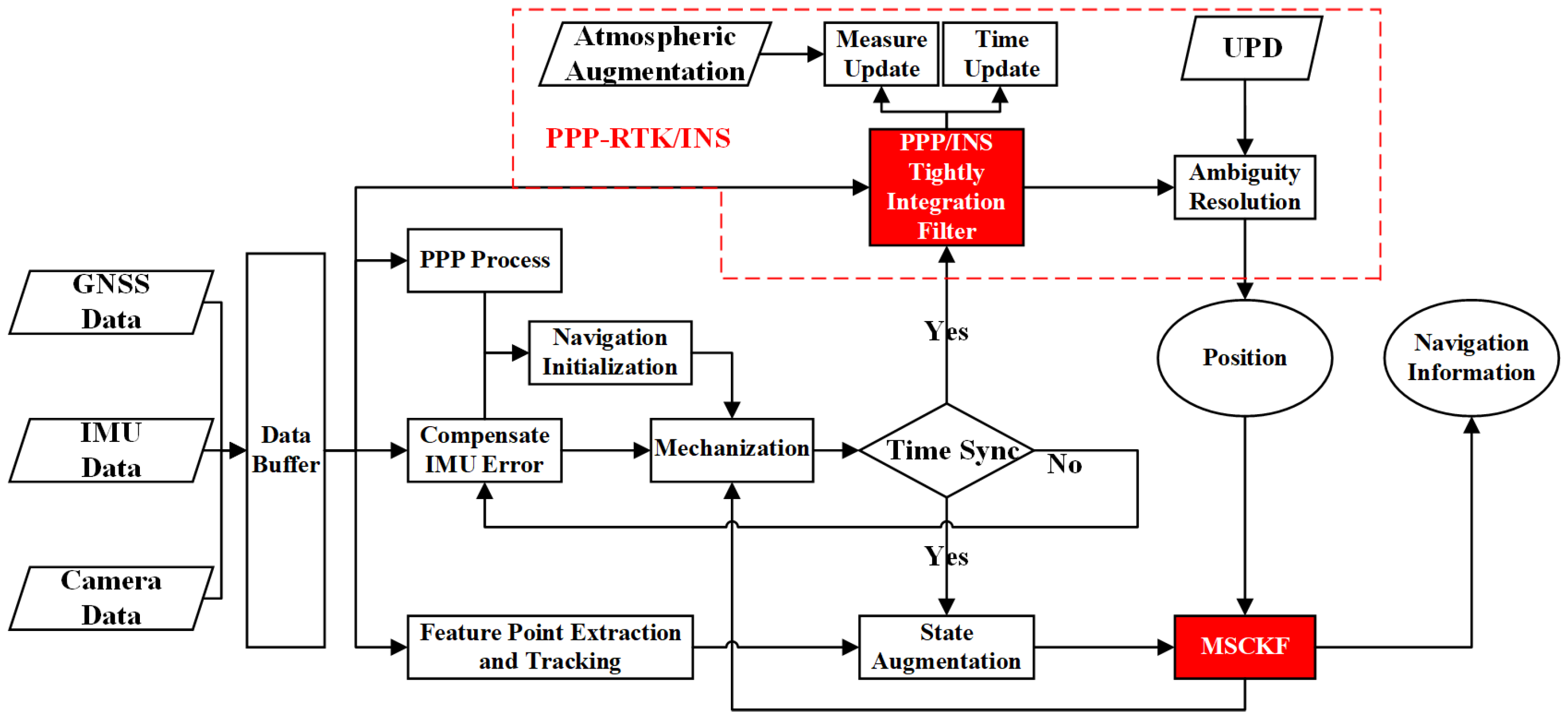
This paper aims to evaluate the navigation performance of the integration of multi-GNSS PPP-RTK, MEMS-IMU, and monocular cameras with a cascading filter and the dynamic object removal algorithm in urban areas. The remainder of this paper is organized as follows: first, Section 2 presents the mathematical models of PPP-RTK, the MEMS-IMU, and monocular camera integration based on the MSCKF, integration of multi-GNSS PPP-RTK, INS, and vision as well as the dynamic object removal model, and introduces the structure of the proposed model. Then, the details of the test are demonstrated in Section 3 and the efficiency of different techniques in urban vehicle navigation is analyzed in Section 4. Finally, Section 5 presents the conclusions.

2. Methods

The undifferenced and uncombined PPP-RTK, INS model, PPP-RTK/INS tightly coupled integration model, as well as the vision model, are presented in this section in order to derive the integration model of multi-GNSS PPP-RTK/INS/vision with a cascading filter. According to the suggestion in RINEX 3.02 (https://kb.igs.org/hc/en-us/articles/115003980628-RINEX-3-02 (accessed on 12 August 2022)), the GPS and BDS systems are denoted as G and C, respectively.

2.1. PPP-RTK Model

The raw observations of the GNSS pseudo-range and carrier phase can be expressed as follows [39]:

$$\left.\begin{array}{c}{P}_{r,f}^s={\rho }_r^s+t_{r,sys}+{\alpha }_r^s{T}_Z+\frac{40.3}{f^2}{\gamma }_r^s{I}_r^s-b^{s,f}+b_{r,f}+{\epsilon }_{\mathit{p}}\\ {\Phi }_{r,f}^s={\rho }_r^s+t_{r,sys}+{\alpha }_r^s{T}_Z-\frac{40.3}{f^2}{\gamma }_r^s{I}_r^s+\lambda N_{r,f}^s+{\epsilon }_{\Phi }\end{array}\right\}$$

(1)

in which $P_{r,f}^s$ and ${\mathsf{\Phi }}_{r,f}^s$ are the pseudo-range and carrier phase at frequency f corresponding to receiver r and satellite s in length units, respectively; ${\rho }_r^s$ is the geometric distance between receiver r and satellite s; $t_{r,sys}$ is the receiver clock error corresponding to the system $sys\in \left(G C\right)$ in the length units, respectively; ${\alpha }_r^s$ and ${\gamma }_r^s$ are the mapping functions of the tropospheric and ionospheric delays, respectively; $T_Z$ and $I_r^s$ stand for the zenith tropospheric delay and the zenith total electron content (TEC); $b^{s,f}$ and $b_{r,f}$ denote the hardware delay for satellite s and receiver r, respectively; $\lambda$ and $N_{r,f}^s$ are the carrier phase wavelength and float ambiguity; ${\epsilon }_{\mathit{p}}$ and ${\epsilon }_{\Phi }$ represent the measurement noise of pseudo-range and carrier phase including the unmodeled multipath error, respectively. Additionally, it is assumed that other errors, such as satellite orbit and clock errors and relativistic effects, are corrected in advance.

After correcting the hardware delay for the satellite and linearization, Equation (1) can be written as

$$\left.\begin{array}{c}\Delta P_{r,f}^s={\mathit{h}}_{\mathit{s}}^{\mathit{r}}\mathit{\delta }{\mathit{x}}_{\mathit{G}\mathit{N}\mathit{S}\mathit{S}}^{\mathit{e}}+t_{r,sys}+{\alpha }_r^s\delta T_w+\frac{40.3}{f^2}{\gamma }_r^s{I}_r^s+b_{r,f}+{\epsilon }_p\\ \Delta {\Phi }_{r,f}^s={\mathit{h}}_{\mathit{s}}^{\mathit{r}}\mathit{\delta }{\mathit{x}}_{\mathit{G}\mathit{N}\mathit{S}\mathit{S}}^{\mathit{e}}+t_{r,sys}+{\alpha }_r^s\delta T_w-\frac{40.3}{f^2}{\gamma }_r^s{I}_r^s+\lambda N_{r,f}^s+{\epsilon }_{\Phi }\end{array}\right\}$$

(2)

where $\mathsf{\Delta }{P}_{r,f}^s$ and ${\mathsf{\Delta }\mathsf{\Phi }}_{r,f}^s$ are the OMC (observed-minus-computed) of the pseudo-range and carrier phase, respectively; superscript ${·}^e$ represents the e-frame (earth-centered earth-fixed frame); $\mathit{\delta }{\mathit{x}}_{\mathit{G}\mathit{N}\mathit{S}\mathit{S}}^{\mathit{e}}$ and ${\mathit{h}}_r^s$ are the correction vectors of the receiver position and the corresponding direction cosine vector; $\mathsf{\delta }{T}_w$ denotes the residual of the zenith tropospheric wet delay. Additionally, the DESIGN (deterministic plus stochastic ionosphere model for GNSS) model is adopted in this study as [39,40]

$$\left.\begin{array}{c}{I}_r^s=a_0+a_{1}dL+a_{2}dB+a_{3}d{L}^2+a_{4}d{B}^2+r_r^s\\ {\tilde{I}}_r^s=a_0+a_{1}dL+a_{2}dB+a_{3}d{L}^2+a_{4}d{B}^2+r_r^s+{\epsilon }_{{\tilde{I}}_r^s}\end{array}\right\}$$

(3)

in which ${\tilde{I}}_r^s$ is the virtual observation of ionospheric delay and can be obtained from the ionospheric delay prior models of high-precision ionospheric products; $a_i$ (i = 0, 1, 2, 3, 4) describes the spatial distribution of the ionospheric delay; and dL and dB represent the difference in longitude and latitude between the approximate location of the station and the ionospheric pierce point (IPP), respectively. $r_r^s$ describes the stochastic behavior of the ionospheric delay in the time domain and ${\epsilon }_{{\tilde{I}}_r^s}$ is the corresponding noise of the virtual observation.

Then, the state vector ${\mathit{x}}_{\mathit{P}\mathit{P}\mathit{P}-\mathit{R}\mathit{T}\mathit{K}}$ can be written as

$${\mathit{x}}_{\mathit{P}\mathit{P}\mathit{P}-\mathit{R}\mathit{T}\mathit{K}}={\left(\begin{array}{cccccc}\mathit{\delta }{\mathit{x}}_{\mathit{G}\mathit{N}\mathit{S}\mathit{S}}^{\mathit{e}}& t_r& \delta T_w& b_r& {\mathit{N}}_{\mathit{r}}& {\mathit{a}}_{\mathit{r}}\end{array}{\mathit{r}}_{\mathit{r}}\right)}^T$$

(4)

where ${\mathit{N}}_{\mathit{r}}={\left(\begin{array}{cc}{\mathit{N}}_{\mathit{r},1}& {\mathit{N}}_{\mathit{r},2}\end{array}\right)}^T$ denotes the float ambiguity on frequency $f_1$ and $f_2$; ${\mathit{a}}_{\mathit{r}}=$ (a₀ a₁ a₂ a₃ a₄)^T and ${\mathit{r}}_{\mathit{r}}={\left(r_r^1\dots r_r^j\right)}^T$ means the deterministic and stochastic parameters of the DESIGN, respectively.

The float ambiguity $N_{r,f}^s$ should be further formulated for the PPP ambiguity resolution. It can be expressed as

$$N_{r,f}^s=n-d_r+d^s$$

(5)

in which $n$ means the integer ambiguity and $d_r$ and $d^s$ are the UPD for the receiver and satellite. After the float ambiguity is obtained by Equation (2), the UPD can be removed and then the integer property of the ambiguity can be recovered. Moreover, the LAMBDA (least-squares ambiguity decorrelation adjustment) method is applied to search for the optimal fixed value of the ambiguity [41]. Finally, the integer ambiguity is used as constraints to obtain the PPP solution with fixed ambiguity.

2.2. INS Model

In this paper, the mechanization is conducted in the e-frame (earth-centered earth-fixed frame) for easily integrating the state of INS with the GNSS observables. Then, the dynamic equation of INS can be described as

$$\left(\begin{array}{c}{\dot{\mathit{x}}}_{\mathit{I}\mathit{N}\mathit{S}}^{\mathit{e}}\\ {\dot{\mathit{v}}}_{\mathit{I}\mathit{N}\mathit{S}}^{\mathit{e}}\\ {\dot{\mathit{C}}}_{\mathit{b}}^{\mathit{e}}\end{array}\right)=\left(\begin{array}{c}{\mathit{v}}_{\mathit{I}\mathit{N}\mathit{S}}^{\mathit{e}}\\ {\mathit{C}}_{\mathit{b}}^{\mathit{e}}{\mathit{f}}^{\mathit{b}}-2{\mathit{\omega }}_{\mathit{i}\mathit{e}}^{\mathit{e}}\times {\mathit{v}}_{\mathit{I}\mathit{N}\mathit{S}}^{\mathit{e}}+{\mathit{g}}^{\mathit{e}}\\ {\mathit{C}}_{\mathit{b}}^{\mathit{e}}\left[{\mathit{\omega }}_{\mathit{e}\mathit{b}}^{\mathit{b}}\times \right]\end{array}\right)$$

(6)

where ${\mathit{x}}_{\mathit{I}\mathit{N}\mathit{S}}^{\mathit{e}}$ is the position vector in the e-frame, respectively; ${\mathit{v}}_{\mathit{I}\mathit{N}\mathit{S}}^{\mathit{e}}$ is the velocity vector in the e-frame; ${\mathit{C}}_{\mathit{b}}^{\mathit{e}}$ represents the rotation matrix from the b-frame (body frame) to the e-frame; ${\mathit{f}}^{\mathit{b}}$ is the specific force vector generated by the accelerometers in the b-frame; ${\mathit{\omega }}_{\mathit{i}\mathit{e}}^{\mathit{e}}$ is the earth rotation vector of the e-frame against the i-frame (inertial frame) in the e-frame; ${\mathit{g}}^{\mathit{e}}$ denotes the local gravity vector in the e-frame; ${\mathit{\omega }}_{\mathit{e}\mathit{b}}^{\mathit{b}}$ denotes the rotation rate vector of the b-frame against the e-frame projected to the b-frame; and $\left[·\times \right]$ denotes the skew-symmetric matrix.

By using the Phi-angle error model, the INS error model can be written as [42]

$$\left(\begin{array}{c}\mathit{\delta }{\dot{\mathit{x}}}_{\mathit{I}\mathit{N}\mathit{S}}^{\mathit{e}}\\ \mathit{\delta }{\dot{\mathit{v}}}_{\mathit{I}\mathit{N}\mathit{S}}^{\mathit{e}}\\ \dot{\mathit{\varphi }}\end{array}\right)=\left(\begin{array}{c}\mathit{\delta }{\mathit{v}}_{\mathit{I}\mathit{N}\mathit{S}}^{\mathit{e}}\\ -2{\mathit{\omega }}_{\mathit{i}\mathit{e}}^{\mathit{e}}\times \mathit{\delta }{\mathit{v}}_{\mathit{I}\mathit{N}\mathit{S}}^{\mathit{e}}+{\mathit{C}}_{\mathit{b}}^{\mathit{e}}{\mathit{f}}^{\mathit{b}}\times \mathit{\varphi }+{\mathit{C}}_{\mathit{b}}^{\mathit{e}}\mathit{\delta }{\mathit{f}}^{\mathit{b}}+\mathit{\delta }{\mathit{g}}^{\mathit{e}} \\ -{\mathit{\omega }}_{\mathit{i}\mathit{e}}^{\mathit{e}}\times \mathit{\varphi }-{\mathit{C}}_{\mathit{b}}^{\mathit{e}}\mathit{\delta }{\mathit{\omega }}_{\mathit{i}\mathit{b}}^{\mathit{b}}\end{array}\right)$$

(7)

in which $\mathit{\varphi }$ indicates the correction vector of attitude; $\mathit{\delta }{\mathit{g}}^{\mathit{e}}$ represents the gravity error in the e-frame; and $\mathit{\delta }{\mathit{f}}^{\mathit{b}}$ and $\mathit{\delta }{\mathit{\omega }}_{\mathit{i}\mathit{b}}^{\mathit{b}}$ are the sensor errors of the accelerometer and gyroscope, respectively. Bias and scale factor errors along with white noise can be used to model the sensor error [42], which can be expressed as

$$\left\{\begin{array}{c}\mathit{\delta }{\mathit{f}}^{\mathit{b}}={\mathit{B}}_{\mathit{a}}+\mathit{diag}\left({\mathit{f}}^{\mathit{b}}\right){\mathit{S}}_{\mathit{a}}+{\mathit{w}}_{\mathit{v}}\\ \mathit{\delta }{\mathit{\omega }}_{\mathit{i}\mathit{b}}^{\mathit{b}}={\mathit{B}}_{\mathit{g}}+\mathit{diag}\left({\mathit{\omega }}_{\mathit{i}\mathit{b}}^{\mathit{b}}\right){\mathit{S}}_{\mathit{g}}+{\mathit{w}}_{\mathit{\varphi }}\end{array}\right.$$

(8)

in which, ${\mathit{B}}_{\mathit{a}}$ and ${\mathit{S}}_{\mathit{a}}$ indicate the bias and scale factor errors of the accelerometer, respectively; $\mathit{diag}$ denotes the diagonal matrix; ${\mathit{B}}_{\mathit{g}}$ and ${\mathit{S}}_{\mathit{g}}$ indicate the bias and scale factor errors of the gyroscope, respectively; and ${\mathit{w}}_{\mathit{v}}$ and ${\mathit{w}}_{\mathit{\varphi }}$ indicate the corresponding random white noise. Bias and scale factor errors can be modeled as first-order Gauss–Markov processes and expressed as [42]

$$\left\{\begin{array}{c}\left(\begin{array}{c}{\dot{\mathit{B}}}_{\mathit{a}}\\ {\dot{\mathit{B}}}_{\mathit{g}}\end{array}\right)=\left(\begin{array}{c}\frac{-1}{{\tau }_{ba}}{\mathit{B}}_{\mathit{a}}\\ \frac{-1}{{\tau }_{bg}}{\mathit{B}}_{\mathit{g}}\end{array}\right)+\left(\begin{array}{c}{\mathit{w}}_{\mathit{b}\mathit{a}}\\ {\mathit{w}}_{\mathit{b}\mathit{g}}\end{array}\right)\\ \left(\begin{array}{c}{\dot{\mathit{S}}}_{\mathit{a}}\\ {\dot{\mathit{S}}}_{\mathit{g}}\end{array}\right)=\left(\begin{array}{c}\frac{-1}{{\tau }_{sa}}{\mathit{S}}_{\mathit{a}}\\ \frac{-1}{{\tau }_{sg}}{\mathit{S}}_{\mathit{g}}\end{array}\right)+\left(\begin{array}{c}{\mathit{w}}_{\mathit{s}\mathit{a}}\\ {\mathit{w}}_{\mathit{s}\mathit{g}}\end{array}\right)\end{array}\right.$$

(9)

where ${\tau }_{\left(\bullet \right)}$ and ${\mathit{w}}_{\left(\bullet \right)}$ (denotes the subscript ba, bg, sa, or sg) denote the corresponding correlation time and driving white noise, respectively.

Finally, the INS error state can be modeled as

$${\mathit{x}}_{\mathit{I}\mathit{N}\mathit{S}}={\left(\begin{array}{cccccc}\mathit{\delta }{\mathit{x}}_{\mathit{I}\mathit{N}\mathit{S}}^{\mathit{e}}& \mathit{\delta }{\mathit{v}}_{\mathit{I}\mathit{N}\mathit{S}}^{\mathit{e}}& \mathit{\varphi }& {\mathit{B}}_{\mathit{a}}& {\mathit{B}}_{\mathit{g}}& {\mathit{S}}_{\mathit{a}}\end{array}{\mathit{S}}_{\mathit{g}}\right)}^T$$

(10)

2.3. PPP-RTK/INS Tightly Coupled Integration Model

In the error state of PPP-RTK and INS, ${\mathit{x}}_{GNSS}^e$ and ${\mathit{x}}_{INS}^e$ denote the position of the GNSS receiver antenna reference point (ARP) and IMU center, respectively. They do not represent the same position and their spatial relationship in the e-frame can be expressed as [42]

$${\mathit{x}}_{\mathit{G}\mathit{N}\mathit{S}\mathit{S}}^{\mathit{e}}={\mathit{x}}_{\mathit{I}\mathit{N}\mathit{S}}^{\mathit{e}}+{\mathit{C}}_{\mathit{b}}^{\mathit{e}}{\mathit{l}}^{\mathit{b}}$$

(11)

in which ${\mathit{l}}^b$ means the lever-arm correction vector in the b-frame. As for the approximate coordinates ${\tilde{\mathit{x}}}_{GNSS}^e$ and ${\tilde{\mathit{x}}}_{INS}^e$, their relationship can be described as

$${\tilde{\mathit{x}}}_{\mathit{G}\mathit{N}\mathit{S}\mathit{S}}^{\mathit{e}}={\tilde{\mathit{x}}}_{\mathit{I}\mathit{N}\mathit{S}}^{\mathit{e}}+{\tilde{\mathit{C}}}_{\mathit{b}}^{\mathit{e}}{\mathit{l}}^{\mathit{b}}$$

(12)

where ${\tilde{\mathit{C}}}_b^e$ is the approximation of ${\mathit{C}}_{\mathit{b}}^{\mathit{e}}$, and satisfies

$${\tilde{\mathit{C}}}_{\mathit{b}}^{\mathit{e}}=\left(\mathit{I}-\mathit{\varphi }\times \right){\mathit{C}}_{\mathit{b}}^{\mathit{e}}$$

(13)

Then, the following equation of $\mathit{\delta }{\mathit{x}}_{GNSS}^e$ and $\mathsf{\delta }{\mathit{x}}_{INS}^e$ can be derived from Equations (11) to (13):

$$\mathit{\delta }{\mathit{x}}_{\mathit{G}\mathit{N}\mathit{S}\mathit{S}}^{\mathit{e}}=\mathit{\delta }{\mathit{x}}_{\mathit{I}\mathit{N}\mathit{S}}^{\mathit{e}}+{\mathit{C}}_{\mathit{b}}^{\mathit{e}}{\mathit{l}}^{\mathit{b}}\times \mathit{\varphi }$$

(14)

The state error in the integrated navigation is defined as the observation minus the true value, whereas the state error in the GNSS is defined as the true value minus the observation. Thus, the signs of $\mathit{\delta }{\mathit{x}}_{\mathit{G}\mathit{N}\mathit{S}\mathit{S}}^{\mathit{e}}$ and $\mathit{\delta }{\mathit{x}}_{\mathit{I}\mathit{N}\mathit{S}}^{\mathit{e}}$ are opposite. After adding a minus sign to Equation (14) and substituting it into Equation (2), the observation equation of the PPP-RTK/INS can be further expressed as

$$\left.\begin{array}{c}\mathsf{\Delta }{P}_{r,f}^s=-{\mathit{h}}_{\mathit{r}}^{\mathit{s}}\mathit{\delta }{\mathit{x}}_{\mathit{I}\mathit{N}\mathit{S}}^{\mathit{e}}-{\mathit{h}}_{\mathit{r}}^{\mathit{s}}{\mathit{C}}_{\mathit{b}}^{\mathit{e}}{\mathit{l}}^{\mathit{b}}\times \mathit{\varphi }+t_{r,sys}+{\alpha }_r^s\mathsf{\delta }{T}_w+b_{r,f}+{\epsilon }_{\mathit{p}}\\ +\frac{40.3}{f^2}{\gamma }_r^s(a_0+a_{1}dL+a_{2}dB+a_{3}d{L}^2+a_{4}d{B}^2+r_r^s+{\epsilon }_{{\tilde{I}}_r^s})\\ {\mathsf{\Delta }\mathsf{\Phi }}_{r,f}^s=-{\mathit{h}}_{\mathit{r}}^{\mathit{s}}\mathit{\delta }{\mathit{x}}_{\mathit{I}\mathit{N}\mathit{S}}^{\mathit{e}}-{\mathit{h}}_{\mathit{r}}^{\mathit{s}}{\mathit{C}}_{\mathit{b}}^{\mathit{e}}{\mathit{l}}^{\mathit{b}}\times \mathit{\varphi }+t_{r,sys}+{\alpha }_r^s\mathsf{\delta }{T}_w+\lambda N_{r,f}^s+{\epsilon }_{\mathsf{\Phi }}\\ -\frac{40.3}{f^2}{\gamma }_r^s(a_0+a_{1}dL+a_{2}dB+a_{3}d{L}^2+a_{4}d{B}^2+r_r^s+{\epsilon }_{{\tilde{I}}_r^s})\\ {\tilde{I}}_r^s=a_0+a_{1}dL+a_{2}dB+a_{3}d{L}^2+a_{4}d{B}^2+r_r^s+{\epsilon }_{{\tilde{I}}_r^s}\end{array}\right\}$$

(15)

Combining the state vector ${\mathit{x}}_{\mathit{P}\mathit{P}\mathit{P}-\mathit{R}\mathit{T}\mathit{K}}$ in Equation (4) and ${\mathit{x}}_{\mathit{I}\mathit{N}\mathit{S}}$ in Equation (10), the state vector of the PPP-RTK/INS can be described as

$$\mathit{x}=({\mathit{\delta }{\mathit{x}}_{\mathit{I}\mathit{N}\mathit{S}}^{\mathit{e}} \mathit{\delta }{\mathit{v}}_{\mathit{I}\mathit{N}\mathit{S}}^{\mathit{e}} \mathit{\varphi } \mathit{B} \mathit{S} t_r \mathsf{\delta }{T}_w b_r {\mathit{N}}_{\mathit{r}} {\mathit{a}}_{\mathit{r}} {\mathit{r}}_{\mathit{r}})}^{\mathit{T}}$$

(16)

2.4. INS/Vision Tightly Coupled Integration Model

By denoting the error state of the camera as $\left(\delta {\mathit{p}}_{c_i}^e {\mathit{\varphi }}_{c_i}\right)$ for the ith image, the error state vector of INS/vision tightly coupled integration with the MSCKF at the time when the kth image is captured is expressed as

$${\mathit{x}}_{i,c}={\left(\begin{array}{cccccc}{\mathit{x}}_{INS}& |& \mathsf{\delta }{\mathit{p}}_{c_j}^e& {\mathit{\varphi }}_{c_j}& \dots & \mathsf{\delta }{\mathit{p}}_{c_k}^e\end{array}{\mathit{\varphi }}_{c_k}\right)}^T$$

(17)

in which $\mathsf{\delta }{\mathit{p}}_{c_i}^e$ and ${\mathit{\varphi }}_{c_i}$ (i = j, j + 1, …, k) indicate the error states of the camera position and attitude for epoch i. The above error state vector is augmented when new camera data is introduced.

Visual measurements of the same feature point from multiple camera views are used to construct the geometric constraints. At the time of taking the ith (i < k + 1) image, the transformation of the static feature point $P_k$ can be expressed as

$${\mathit{p}}_{P_k,i}^{c_i}={\mathit{R}}_e^{c_i}\left({\mathit{p}}_{P_k}^e-{\mathit{p}}_{c_i}^e\right)$$

(18)

in which, ${\mathit{p}}_{P_k,i}^{c_i}=\left(\begin{array}{ccc}{x}_{P_k,i}^{c_i}& y_{P_k,i}^{c_i}& z_{P_k,i}^{c_i}\end{array}\right)$ indicates the position of $P_k$ in the camera frame; ${\mathit{R}}_e^{c_i}$ and ${\mathit{p}}_{c_i}^e$ are the attitude rotation matrix and position vector against the global frame (e-frame), respectively; ${\mathit{p}}_{P_k}^e$ is the estimated position of $P_k$ in the e-frame, which can be calculated by triangulation. By differentiating Equation (18), the equation of the camera state can be obtained as follows:

$$\delta {\mathit{p}}_{P_k,i}^{c_i}=-{\mathit{R}}_e^{c_i}\left[\left({\mathit{p}}_{P_k}^e-{\mathit{p}}_{c_i}^e\right)\times \right]{\mathit{\varphi }}_{c_i}-{\mathit{R}}_e^{c_i}\delta {\mathit{p}}_{c_i}^e+{\mathit{R}}_e^{c_i}\delta {\mathit{p}}_{P_k}^e$$

(19)

in which $\delta {\mathit{p}}_{P_k}^e$ indicates the error of the approximate position of the feature point.

Concerning the camera measurement residual vector, it can be written as

$$z_{P_k,i}=\left(\begin{array}{c}{u}_{P_k,i}^0-{\tilde{u}}_{P_k,i}\\ v_{P_k,i}^0-{\tilde{v}}_{P_k,i}\end{array}\right), {\epsilon }_{P_k,i}=\left(\begin{array}{c}{\epsilon }_{{\tilde{u}}_{P_k,i}}\\ {\epsilon }_{{\tilde{v}}_{P_k,i}}\end{array}\right)$$

(20)

where ${(u_{P_k,i}^0,v_{P_k,i}^0)}^T$ is the estimated pixel coordinate of $P_k$ by back projection and ${({\tilde{u}}_{P_k,i},{\tilde{v}}_{P_k,i})}^T$ is the observation of $P_k$ in the ith image and ${\mathit{\epsilon }}_{P_k,i}$ is the measurement noise. Then, based on the chain rule, the residual formula can be expressed as [27]

$${\mathit{z}}_{P_k,i}=\delta {\left(u_{P_k,i},v_{P_k,i}\right)}^T=\frac{\partial {\left(u_{P_k,i},v_{P_k,i}\right)}^T}{\partial {\mathit{p}}_{P_k,i}^{c_i}}\delta {\mathit{p}}_{P_k,i}^{c_i}={\mathit{H}}_{x,i}{\mathit{x}}_{i,c}+{\mathit{H}}_{f,i}\delta {\mathit{p}}_{P_k}^e+{\mathit{\epsilon }}_{P_k,i}$$

(21)

where

$$\begin{gathered} {\mathit{H}}_{x,i}=\left(\begin{array}{cccccc}{0}_{2\times 21}& 0_{2\times 6}& \dots & -\mathit{J}{\mathit{R}}_e^{c_i}& -\mathit{J}{\mathit{R}}_e^{c_i}\left[\left({\mathit{p}}_{P_k}^e-{\mathit{p}}_{c_i}^e\right)\times \right]& \dots \end{array}\right) \\ {\mathit{H}}_{f,i}=\mathit{J}{\mathit{R}}_e^{c_i} \\ \mathit{J}=\frac{\partial {\left(u_{P_k,i},v_{P_k,i}\right)}^T}{\partial {\mathit{p}}_{P_k,i}^{c_i}}=\left(\begin{array}{ccc}\frac{f_x}{z_{P_k,i}^{c_i}}& 0& -\frac{f_x{x}_{P_k,i}^{c_i}}{z_{P_k,i}^{c_i}{}^2}\\ 0& \frac{f_y}{z_{P_k,i}^{c_i}}& -\frac{f_y{y}_{P_k,i}^{c_i}}{z_{P_k,i}^{c_i}{}^2}\end{array}\right) \end{gathered}$$

in which $(f_x,f_y)$ means the focal length and $\left(\begin{array}{ccc}{x}_{P_k,i}^{c_i}& y_{P_k,i}^{c_i}& z_{P_k,i}^{c_i}\end{array}\right)$ means the position of a feature point in the camera frame.

Because $\delta {\mathit{p}}_{P_k}^e$ is not the state that needs to be estimated and ${\mathit{H}}_{f,i}$ is known, we can calculate the left null space A, which satisfies the equation as follows:

$${\mathit{A}}^T{\mathit{H}}_{f,i}=0$$

(22)

Then, multiplying ${\mathit{A}}^T$ at both sides of Equation (21), the measurement model can be described as

$${\mathit{z}}_{a,i}={\mathit{A}}^T{\mathit{z}}_{P_k,i}={\mathit{A}}^{\mathit{T}}{\mathit{H}}_{\mathit{x},\mathit{i}}{\mathit{x}}_{\mathit{i},\mathit{c}}+{\mathit{A}}^T{\mathit{\epsilon }}_{P_k,i}={\mathit{H}}_{a,x,i}{\mathit{x}}_{i,c}+{\mathit{\epsilon }}_{a,i}$$

(23)

where ${\mathit{z}}_{a,i}={\mathit{A}}^T{\mathit{z}}_{P_k,i}$, ${\mathit{H}}_{a,x,i}={\mathit{A}}^T{\mathit{H}}_{x,i}$ and ${\mathit{\epsilon }}_{a,i}={\mathit{A}}^T{\mathit{\epsilon }}_{P_k,i}$, respectively.

The pixel coordinate of $P_k$ can be described as follows:

$$\left(\begin{array}{c}{\tilde{u}}_{P_k,i}\\ {\tilde{v}}_{P_k,i}\\ 1\end{array}\right)=\frac{1}{z_{P_k,i}^{c_i}}K{\mathit{p}}_{P_k,i}^{c_i}$$

(24)

in which K denotes the camera intrinsic parameter.

Substituting Equation (18) into (25), we have:

$$\left(\begin{array}{c}{\tilde{u}}_{P_k,i}\\ {\tilde{v}}_{P_k,i}\\ 1\end{array}\right)=\frac{1}{z_{P_k,i}^{c_i}}K{\mathit{R}}_e^{c_i}\left({\mathit{p}}_{P_k}^e-{\mathit{p}}_{c_i}^e\right)$$

(25)

Thus,

$$\left(\begin{array}{c}∆{\tilde{u}}_{P_k}\\ ∆{\tilde{v}}_{P_k}\\ 0\end{array}\right)=K\left[\frac{1}{z_{P_k,i+1}^{c_{i+1}}}{\mathit{R}}_e^{c_{i+1}}\left(\acute{{\mathit{p}}_{P_k}^e}-{\mathit{p}}_{c_{i+1}}^e\right)-\frac{1}{z_{P_k,i}^{c_i}}{\mathit{R}}_e^{c_i}\left({\mathit{p}}_{P_k}^e-{\mathit{p}}_{c_i}^e\right)\right]$$

(26)

where $∆{\tilde{u}}_{P_k}={\tilde{u}}_{P_k,i+1}-{\tilde{u}}_{P_k,i}$, $∆{\tilde{v}}_{P_k}={\tilde{v}}_{P_k,i+1}-{\tilde{v}}_{P_k,i}$. $\acute{{\mathit{p}}_{P_k}^e}$ is the position of $P_k$ for the epoch i+1. ${({\tilde{u}}_{P_k,i+1},{\tilde{v}}_{P_k,i+1})}^T$ is the observation of $P_k$ in the i+1th image.

Considering that the time interval is relatively small, we assume that the pose and position of the camera have no obvious changes. Because $z_{P_k,i+1}^{c_{i+1}}$ is relatively large, we can make assumptions: ${\mathit{R}}_e^{c_{i+1}}\approx {\mathit{R}}_e^{c_i}$, $\frac{1}{z_{P_k,i+1}^{c_{i+1}}}\approx \frac{1}{z_{P_k,i}^{c_i}}$. For the static feature point, ${\mathit{p}}_{P_k}^e-\acute{{\mathit{p}}_{P_k}^e}$ = 0, thus we can obtain

$$z_{P_k,i+1}^{c_{i+1}}\left(\begin{array}{c}∆{\tilde{u}}_{P_k}\\ ∆{\tilde{v}}_{P_k}\\ 0\end{array}\right)=-K{\mathit{R}}_e^{c_{i+1}}\left({\mathit{p}}_{c_{i+1}}^e-{\mathit{p}}_{c_i}^e\right)$$

(27)

As we know, ${\mathit{p}}_{c_{i+1}}^e$ and ${\mathit{p}}_{c_i}^e$ can be obtained by PPP-RTK/INS. For dynamic objects on the road, [$\left({\mathit{p}}_{P_k}^e-{\mathit{p}}_{c_{i+1}}^e\right)$ − $\left(\acute{{\mathit{p}}_{P_k}^e}-{\mathit{p}}_{c_i}^e\right)]<\left({\mathit{p}}_{c_{i+1}}^e-{\mathit{p}}_{c_i}^e\right)$. By setting a threshold for $z_{P_k,i+1}^{c_{i+1}}$, the dynamic objects can be removed.

2.5. PPP-RTK/INS/Vision Integration Model with a Cascading Filter

The PPP-RTK/INS/vision integration model with a cascading filter is realized by integrating the output of the tightly coupled integration of PPP-RTK/INS with the tightly coupled integration of INS/vision. The difference between the position provided by the PPP-RTK/INS and the position predicted by INS/vision constitutes the observation of position. Based on Equations (14) and (23), the measurement model of the PPP-RTK/INS/Vision integration model can be expressed as

$$\left.\begin{array}{c}{\widehat{\mathit{x}}}_{GNSS}^e-{\tilde{\mathit{x}}}_{GNSS}^e=\mathit{\delta }{\mathit{x}}_{\mathit{I}\mathit{N}\mathit{S}}^{\mathit{e}}+{\mathit{C}}_b^e{\mathit{l}}^b\times \mathit{\varphi }+{\mathit{\epsilon }}_{\mathit{x}}\\ {\mathit{z}}_{a,i}={\mathit{H}}_{a,\mathit{x},i}{\mathit{x}}_{i,c}+{\mathit{\epsilon }}_{a,i}\end{array}\right\}$$

(28)

in which ${\widehat{\mathit{x}}}_{GNSS}^e$ is the position predicted by INS/vision and ${\tilde{\mathit{x}}}_{GNSS}^e$ is the positioning results of PPP-RTK/INS. ${\mathit{\epsilon }}_{\mathit{x}}$ is the measurement noise.

The integration model of multi-GNSS PPP-RTK/INS/vision with a cascading filter is derived from the description above. An overview of the proposed model is shown in Figure 1. First, the position is obtained by the GNSS to assist the navigation initialization, e.g., IMU alignment with GNSS. Then, the INS begins to provide high-rate navigation. When the INS synchronizes with the GNSS, tightly coupled integration is performed based on either PPP/INS or PPP-RTK/INS. As for the latter, high-precision atmospheric correction is applied and AR is carried out with the UPD products. Furthermore, feature points are extracted and tracked in each image. When the time of the camera synchronizes with the INS, the state vector is augmented and the MSCKF is adopted to calculate the relative position of the vehicle platform. The positioning results of the GNSS/INS are then integrated with the MSCKF to produce the final navigation information. There are two Kalman filters: the filter of PPP-RTK/INS and the filter of INS/Vision. The positioning results of PPP-RTK/INS are added into the filter of the INS/vision so it becomes a cascading Kalman filter. All the IMU sensor errors are fed back in time in the process.

3. Experiment

To evaluate the positioning accuracy and performance of the proposed integration model of multi-GNSS PPP-RTK/INS/vision with a cascading filter in urban areas, based on the FUSING (FUSing IN Gnss) software [7,40,41], this algorithm was further developed by us. At present, FUSING has been developed into an integrated software platform that can deal with real-time multi-GNSS precise orbit determination, atmospheric delay modeling and monitoring, satellite clock estimation, as well as multi-sensor fusion navigation.

Two datasets were collected based on a vehicle platform as shown in Figure 2. One is in the suburban area of Wuhan City on 1 January 2020, and the other is on the Second Ring Road of Wuhan city on 2 January 2020. For simplicity, according to the DOY (day of the year), the two-vehicle tests are denoted as T01 and T02, respectively.

As shown in Figure 2, the raw data was collected by the IMU of two different grades. A MEMS-grade IMU was used to integrate with PPP-RTK and vision to evaluate the performance of the proposed model. The navigation-grade IMU is of high accuracy and is integrated with RTK to calculate the reference solution, which was regarded as the true value. Both IMUs collected the data at a sampling rate of 200 Hz and their performance parameters are listed in

Table 1. Performance parameters of the IMU sensors.

IMU Sensors	Random Walk		Bias
	Velocity ($m/s/\sqrt{h}$)	Angular ($°/\sqrt{h}$)	Gyro. ($°/h$)	Acce. (mGal)
MEMS-grade	0.03	0.17	8	200
Navigation-grade	0.03	0.003	0.027	15

. The grayscale Basler acA640-90gm camera was equipped to collect the raw images at a sampling rate of 10 Hz with a resolution of 659 × 494. The UBLOX-M8T was used for generating the pulses per second (PPS) to trigger the camera exposure and it also recorded the time of the pulse at the same time. GNSS data were collected by Trimble Net R9 at a sampling rate of 1 Hz. The camera-IMU extrinsic parameters were calibrated offline by utilizing the Kalibr tool (https://github.com/ethz-asl/kalibr/ (accessed on 3 January 2020)). The lever-arm correction vector was measured manually.

The test trajectory and the true scenarios for these two tests are shown in the left and right panels of Figure 3, respectively. It can be seen that dataset T01 was collected in a relatively open sky and only a few obstacles were blocking the GNSS signals. T02 was collected in a GNSS-challenged environment and there were many tall buildings on both sides of the narrow road, including some viaducts and tunnels, which could have totally blocked the GNSS signals. The vehicle speeds of T01 and T02 were about 10 m/s and 15 m/s, respectively, which is shown in Figure 4. It can be seen that there were significant changes in velocity and direction. The number of visible satellites and the PDOP (precision dilution of positioning) with a cutoff angle of 10° are shown in Figure 5. Taking, for instance, the GPS, the average number of tracking satellites of T01 and T02 were 9 and 7, respectively, and the average PDOP values were 1.8 and 10.9, respectively, which demonstrates the difference in the observation environment between T01 and T02.

Considering the high-precision ionospheric and tropospheric delay augmentation and ambiguity resolution to support PPP-RTK, the measurement data of seven reference stations as distributed in Figure 6 were also collected. They were processed to generate high-precision atmospheric delay corrections and UPD products. The average distance between the seven reference stations is 40 km and the green trajectories are the trajectories of the two tests as shown in Figure 3.

The details of the GNSS data processing strategy are presented in

Table 2. GNSS data processing strategy of PPP and PPP-RTK.

Items	PPP	PPP-RTK
Ambiguity	float	fixed
Troposphere	GPT2w model and VMF1_HT [43] and the residuals are estimated as random walk	regional model
Ionosphere	DESIGN-5 model [44] with GIM served as a prior constraint	regional model
Observation model	undifferenced and uncombined
Frequency band	GPS: L1/L2; BDS: B1/B2
Cutoff angle	10°
PCO/PCV	igs14.atx
Solid earth tides	IERS 2010
Receiver clock	estimated as white noise
Ephemeris	precise products provided by GFZ
Code bias	receiver: estimated as random walk; satellite: corrected with IGS product
Sigma of code	0.3 m
Sigma of phase	0.003 m

. The positioning performance was evaluated by RMS (root mean square). The reference solution was calculated by a loosely coupled RTK/INS solution with a bi-directional smoothing algorithm, in which navigation-grade IMU and GNSS data collected by Trimble R9 were adopted. The ground truth was calculated using commercial software named GINS (http://www.whmpst.com/cn/ (accessed on 15 April 2021)). The nominal positioning accuracy of the RTK/INS loosely coupled solution provided by GINS was at the level of 2 cm for horizontal and 3 cm for vertical.

4. Results

All results were output at a frequency of 1 Hz. In the following analysis, PPP-RTK/INS means the tightly coupled integration of PPP-RTK and INS. PPP-RTK/INS/vision means the integration of PPP-RTK, INS, and vision with a cascading filter. Before analyzing the performance of our proposed integration system in urban areas, the effects of the dynamic feature point removal algorithm aided by position are presented in Figure 7. It can be seen that the feature points on the car (in the red box) were removed. Some points that were extracted from unobvious places were also removed and the most static obvious feature points were saved, which can be used for visual localization. Figure 8 shows the positioning results of PPP-RTK/INS/vision for T02 before and after dynamic feature point removal. The positioning accuracy was improved by dynamic feature point removal, which is demonstrated in the green box in Figure 8. When PPP-RTK/INS provided stable, high-accuracy position information, the error caused by the dynamic feature points was constrained. However, the positioning performance was obviously influenced by the dynamic feature points when the GNSS signals were interfered with. Combining Figure 5 and Figure 8, the GNSS observation conditions were poor and PPP-RTK/INS performed poorly in positioning around time 362,900 s, 364,000 s, and 364,600 s, thus PPP-RTK/INS was not able to restrain the interference of the dynamic feature points. Therefore, the dynamic feature points removal algorithm based on position improved the positioning accuracy when the GNSS signals were severely disturbed. The statistics of the positioning results show that the positioning accuracy was improved by 3 cm and 1 cm in the horizontal and vertical directions, respectively.

The comparison of the performance of different positioning solutions is presented in Figure 9 and Figure 10 for T01 and T02, respectively. It can be seen in the left section in Figure 9 that PPP-RTK converged much faster than PPP, though the ambiguity sometimes failed to fix. It took about 30 s to converge for PPP-RTK and more than 10 min for PPP. Moreover, PPP-RTK had higher accuracy than PPP after convergence. The inclusion of BDS made the series more stable, especially for the vertical direction. Although the contribution of the INS was rather limited in the horizontal direction as shown in the GC-PPP-RTK/INS solution, the outliers may have been inhibited, e.g., around the time 28,400 s. As for the vertical direction, the INS significantly contributed to the improvement of the positioning accuracy. The INS helped the GNSS to converge to and maintain a higher level of positioning accuracy. Additionally, the introduction of vision reduced the fluctuation, although overall, there was no big difference. As for T02, there was no obvious convergence in Figure 10 as the observation environment was complicated and the positioning accuracy was relatively low. However, it still can be seen in the left section in Figure 10 that PPP-RTK performed better than PPP. In order to further demonstrate the convergence and reconvergence effects of PPP and PPP-RTK, enlarged images of parts of Figure 10 are shown in Figure 11 and the correspondence can be seen from the time of the week. PPP-RTK converged and reconverged much faster than PPP and achieved higher positioning accuracy, though the observational environment was challenging. Figure 10 shows that the series of G-PPP and G-PPP-RTK were interrupted many times because the GNSS signals were blocked out, which is embodied in the tracking number of the visible satellites in Figure 5. Both the continuity and accuracy of the positioning were improved with the BDS included. However, the GNSS was still unable to provide positioning results from 362,906 s to 362,965 s because the vehicle was in the tunnel at that time and there was no GNSS signal at all. GC-PPP-RTK/INS provided continuous and more stable positioning information with the integration with the INS, but there was also obvious fluctuation and the existence of epochs with large positioning errors. The positioning errors diverged to 21.74 m, 15.82 m, and 3.82 m in the north, east, and down directions, respectively. The three-dimensional positioning error at 362,965 s was 27.16 m, which is not suitable for vehicle navigation. Furthermore, the positioning error was obviously reduced when vision was included, especially around the time of the week at 362,900 s, 363,600 s, and 364,000 s. The cumulative errors of the INS were effectively constrained by vision. Thus, in the period from 362,906 s to 362,965 s, the maximum errors of the INS/vision were −1.43 m, −3.94 m, and 2.50 m in the north, east, and down directions, respectively. The corresponding three-dimensional error was 4.88 m, which was 0.49% of the traveled distance. It can be concluded that the integration of multi-GNSS PPP-RTK/INS/vision with a cascading filter performed best in comparison with the other four solutions.

The statistics of the position difference between T01 and T02 are presented in

Table 3. RMS of the positioning error of T01 in horizontal and vertical directions, respectively.

Solution	Horizontal [m]	Improvement	Vertical [m]	Improvement	Availability
G-PPP	0.37		0.35		100%
G-PPP-RTK	0.09	75.7%	0.26	25.7%	100%
GC-PPP-RTK	0.09	75.7%	0.22	37.1%	100%
GC-PPP-RTK/INS	0.08	78.4%	0.09	74.3%	100%
GC-PPP-RTK/INS/Vision	0.08	78.4%	0.09	74.3%	100%

and

Table 4. RMS of the positioning error of T02 in horizontal and vertical directions, respectively.

Solution	Horizontal [m]	Improvement	Vertical [m]	Improvement	Availability
G-PPP	1.61		2.40		90.5%
G-PPP-RTK	1.55	3.7%	2.30	4.2%	90.5%
GC-PPP-RTK	0.70	56.5%	1.16	51.7%	95.1%
GC-PPP-RTK/INS	1.84	−14.3%	0.98	59.2%	100%
GC-PPP-RTK/INS/Vision	0.83	48.4%	0.91	62.1%	100%

to further verify the conclusion. Additionally, the number of epochs at which the position information can be obtained is denoted as A and the number of total epochs is denoted as B. Then the positioning availability can be defined as A/B, which is also included in the tables. The improvement statistics are derived in comparison with the G-PPP solution. The statistics show that the PPP-RTK performed better than PPP in both tests. The ambiguity could not be fixed in many epochs for the frequent GPS signal interruptions and disturbances in T02. Thus, the improvement brought by PPP-RTK for T02 was not as obvious as for T01. The horizontal and vertical positioning RMS of the GC-PPP-RTK/INS/vision solution for the test T01 were 0.08 m and 0.09 m, respectively. As for T02, the horizontal and vertical RMS of the GC-PPP-RTK/INS/vision solution were 0.83 m and 0.91 m, respectively. It can be seen that GC-PPP-RTK/INS/vision made significant improvements compared with the other four solutions. The improvements should have been more obvious because of the interruption in G-PPP and G-PPP-RTK. The positioning availabilities of G-PPP and G-PPP-RTK were both 90.5%. The availability increased to 95.1% with the inclusion of BDS, which means that more epochs of worse positioning were taken into consideration. Because of the accumulation errors of the INS, the statistics of GC-PPP-RTK/INS were worse than all the other solutions in the horizontal direction. The statistics of GC-PPP-RTK, GC-PPP-RTK/INS, and GC-PPP-RTK/INS/vision are shown in

Table 5. RMS of the position difference of T02 with part of the epoch excluded in horizontal and vertical directions, respectively.

Solution	Horizontal [m]	Improvement	Vertical [m]	Improvement
GC-PPP-RTK	0.70		1.16
GC-PPP-RTK/INS	0.48	31.4%	0.73	37.1%
GC-PPP-RTK/INS/Vision	0.44	37.1%	0.67	42.2%

, in which the positioning results derived by the INS and vision are excluded, in order to better show the improvements brought by the INS and vision to the positioning performance of GC-PPP-RTK. The improvement statistics were derived in comparison with the GC-PPP-RTK solution. It can be seen that the INS improved the performance of GC-PPP-RTK by 31.4% and 37.1% in the horizontal and vertical directions, respectively. Eventually, the inclusion of vision increased the improvements to 37.1% and 42.2% in the horizontal and vertical directions, respectively.

Position, velocity, and attitude are of great importance for vehicle navigation in urban areas. The velocity error series of GC-PPP-RTK/INS and GC-PPP-RTK/INS/vision for T01 and T02 are shown in Figure 12 and Figure 13, respectively. As dataset T01 was collected in a relatively open-sky environment, the error series was very stable. There was no obvious difference between GC-PPP-RTK/INS and GC-PPP-RTK/INS/vision. Because T02 was collected in a GNSS-challenged environment, there were obvious divergences in the velocity estimation around 362,900 s, 363,600 s, and 364,000 s. The inclusion of vision weakened the impact and improved the accuracy of the velocity estimation in three directions. It can be seen from the statistics in

Table 6. RMS of the velocity error of T01 in north, east, and down directions, respectively.

Solution	North [m/s]	East [m/s]	Down [m/s]	Improvement
GC-PPP-RTK/INS	0.01	0.01	0.02
GC-PPP-RTK/INS/Vision	0.01	0.01	0.01	0%	0%	50.0%

and

Table 7. RMS of the velocity error of T02 in north, east, and down directions, respectively.

Solution	North [m/s]	East [m/s]	Down [m/s]	Improvement
GC-PPP-RTK/INS	0.12	0.07	0.07
GC-PPP-RTK/INS/Vision	0.03	0.05	0.05	75.0%	28.6%	28.6%

that vision could not bring about obvious improvements in an open-sky environment but greatly improved the velocity estimation accuracy in a GNSS-challenged environment. The error of velocity estimation in T02 was reduced by the inclusion of vision from 0.12 m/s, 0.07 m/s, and 0.07 m/s to 0.03 m/s, 0.05 m/s, and 0.05 m/s in the north, east, and down directions, respectively. The improvement in all three directions was more than 20%.

The attitude error series of GC-PPP-RTK/INS and GC-PPP-RTK/INS/vision for T01 and T02 are shown in Figure 14 and Figure 15, respectively. It can be seen that there was no obvious difference between GC-PPP-RTK/INS and GC-PPP-RTK/INS/vision in the roll and pitch angles in T01. As for T02, the error of pitch and yaw angle of GC-PPP-RTK/INS accumulated when GNSS signals were blocked or interfered with. Figure 15 shows that vision helped to constrain the error divergence around 363,000 s when the GNSS signals were blocked, but there was no obvious difference in the roll and pitch angles at other parts in T02. However, the estimation accuracy of the yaw angle was significantly improved with vision aiding in both tests. The statistics of the attitude error are listed in

Table 8. RMS of the attitude error of T01 for GC-PPP-RTK/INS and GC-PPP-RTK/INS/vision.

Solution	Roll [°]	Pitch [°]	Yaw [°]	Improvement
GC-PPP-RTK/INS	0.05	0.04	0.24
GC-PPP-RTK/INS/Vision	0.05	0.04	0.11	0%	0%	54.2%

and

Table 9. RMS of the attitude error of T02 for GC-PPP-RTK/INS and GC-PPP-RTK/INS/vision.

Solution	Roll [°]	Pitch [°]	Yaw [°]	Improvement
GC-PPP-RTK/INS	0.07	0.06	0.39
GC-PPP-RTK/INS/Vision	0.05	0.06	0.26	28.6%	0%	33.3%

. The inclusion of vision reduced the error of the yaw angle from 0.24° to 0.11° and from 0.39° to 0.26° for T01 and T02, respectively. The improvement rates were more than 30% in both tests.

5. Discussion

GC-PPP-RTK/INS/vision integration with a cascading filter can provide continuous positioning information with high precision. The improvements brought about by vision are more significant in challenging environments. Vision reduces the error divergence of PPP-RTK/INS when the GNSS signals are blocked. The positioning error of PPP-RTK/INS reaches 27.16 m after the GNSS signals were lost for 60 s. The inclusion of vision reduces the positioning error to 4.88 m. Vision also helps to improve the estimation accuracy of velocity and attitude. Although the improvements are significant, the positioning accuracy still needs to be improved for vehicle navigation.

Dynamic objects can seriously affect the positioning performance of vision, so it is important to weaken the influence of dynamic objects. The dynamic object removal algorithm proposed in this paper can remove most fast-moving objects and can improve the positioning accuracy of vision. However, it is difficult to deal with slow-moving objects, which is worth further research.

Only GPS and BDS-2 were used in our test so the inclusion of BDS-3 and other systems will be the subject of further research. The integration model of PPP-RTK/INS/vision proposed in this paper is realized by a cascading filter, which can still work when one subsystem is seriously disturbed. The tightly coupled integration of PPP-RTK/INS/vision is another integration method that is worth studying. Because the update frequency of vision is higher, the tightly coupled integration of PPP-RTK/INS/vision may face a heavier computing burden. Therefore, there are still many problems worthy of study in the integration of PPP-RTK/INS/vision.

6. Conclusions

To improve the position, velocity, and attitude estimation performance in urban areas for vehicle navigation, a multi-GNSS PPP-RTK/INS/vision integration model with a cascading filter was developed and validated using two vehicular tests, T01 and T02, in urban areas. T01 was conducted in the suburban area of Wuhan City and T02 on the Second Ring Road of Wuhan city. The T02 test can be regarded as a typical GNSS-challenged environment. To obtain the atmospheric corrections and UPD products for PPP-RTK, observations from seven reference stations were also collected for generating those products.

A dynamic object removal model was also proposed and validated with T02. A dynamic object removal model based on position can work well in a GNSS-challenged environment and improve the positioning performance of multi-GNSS PPP-RTK/INS/vision.

PPP-RTK achieved centimeter-level positioning in the horizontal direction and decimeter-level positioning in the vertical direction under a relatively open sky environment such as T01. The performance in the vertical direction was obviously improved when BDS was included with respect to G-PPP-RTK. Moreover, it took only about 30 s for PPP-RTK convergence due to the atmospheric augmentation and ambiguity resolution. However, incorrect ambiguity resolution remained and the position performance became significantly worse in this case. The introduction of the INS weakened the influence of the incorrect ambiguity resolution and improved the positioning accuracy. The positioning error of GC-PPP-RTK/INS was 0.08 m and 0.09 m, with an improvement of 11.1% and 59.1% in the horizontal and vertical directions, respectively, in comparison with GC-PPP-RTK.

The performance of PPP-RTK degraded fast when the GNSS observation environments became complicated and challenging such as T02. G-PPP-RTK could only achieve meter-level positioning in a GNSS-challenged environment. Compared with G-PPP-RTK, the positioning availability was improved from 90.5% to 95.1% for GC PPP-RTK. The GC-PPP-RTK/INS solution, in comparison with the GC-PPP-RTK solution, contributed significantly to the improvement of the positioning accuracy in the horizontal and vertical directions and the positioning availability. The positioning availability of GC-PPP-RTK/INS increased to 100%. The positioning error of GC-PPP-RTK/INS was 0.48 m and 0.73 m in the horizontal and vertical directions, respectively, after excluding the positioning results derived by the INS. The improvements were 31.4% and 37.1% in the horizontal and vertical directions, respectively, in comparison with GC-PPP-RTK.

The two-vehicle tests showed that GC-PPP-RTK/INS could realize high-precision continuous positioning in a relatively open-sky environment but the positioning errors diverged to more than 20 m in a GNSS-challenged environment. Thus, it needed other sensors such as vision to help restrict the error divergence. Vision did not improve the positioning accuracy statistically but further reduced the fluctuation slightly in the vertical direction for T01. The results indicated that the position RMS of the GC-PPP-RTK/INS/vision tightly coupled integration were 0.08 m and 0.09 m in the horizontal and vertical directions, respectively, which could fully meet the demands of vehicle navigation in urban areas. However, the introduction of vision significantly improved the positioning performance in both the horizontal and vertical directions for T02. The RMS of GC-PPP-RTK/INS/vision reached 0.83 m and 0.91 m in the horizontal and vertical directions, respectively. It improved the positioning accuracy by 54.9% and 7.1% in the horizontal and vertical directions, respectively, compared with GC-PPP-RTK/INS. Additionally, the velocity and attitude estimation performance were also analyzed in this paper. The inclusion of vision improved the velocity performance by more than 25% in the north, east, and down directions in a GNSS-challenged environment. As for attitude, there was no obvious difference with vision in the roll and pitch angles, but GC-PPP-RTK/INS/vision performed much better in the estimation of the yaw angle. The improvements brought about by vision were more than 30% in both tests.

The results show that GC-PPP-RTK/INS/vision integration with a cascading filter performs best in the position, velocity, and attitude estimations compared with the other solutions. Multi-GNSS, INS, and vision can play their respective roles and achieve complementary advantages in vehicle navigation in urban areas. However, navigation performance in real-time still deserves further study.

References

1. Gakne, P.; O’Keefe, K. Tightly-Coupled GNSS/Vision Using a Sky-Pointing Camera for Vehicle Navigation in Urban Areas. Sensors 2018, 18, 1244. [Google Scholar] [CrossRef] [PubMed]
2. Won, D.H.; Lee, E.; Heo, M.; Lee, S.; Lee, J.; Kim, J.; Sung, S.; Lee, Y.J. Selective Integration of GNSS, Vision Sensor, and INS Using Weighted DOP Under GNSS-Challenged Environments. IEEE Trans. Instrum. Meas. 2014, 63, 2288–2298. [Google Scholar] [CrossRef]
3. Mostafa, M.M.; Moussa, A.M.; EI-Sheimy, N.; Sesay, A.B. A smart hybrid vision aided inertial navigation system approach for UAVs in a GNSS denied environment. Navigation 2018, 65, 533–547. [Google Scholar] [CrossRef]
4. Yue, Z.; Lian, B.; Tang, C.; Tong, K. A novel adaptive federated filter for GNSS/INS/VO integrated navigation system. Meas. Sci. Technol. 2020, 31, 085102. [Google Scholar] [CrossRef]
5. Zumberge, J.F.; Heflin, M.B.; Jefferson, D.C.; Watkins, M.M.; Webb, F.H. Precise point positioning for the efficient and robust analysis of GPS data from large networks. J. Geophys. Res. Solid Earth 1997, 102, 5005–5017. [Google Scholar] [CrossRef]
6. Kouba, J.; Héroux, P. Precise Point Positioning Using IGS Orbit and Clock Products. GPS Solut. 2001, 5, 12–28. [Google Scholar] [CrossRef]
7. Shi, C.; Guo, S.; Gu, S.; Yang, X.; Gong, X.; Deng, Z.; Ge, M.; Schuh, H. Multi-GNSS satellite clock estimation constrained with oscillator noise model in the existence of data discontinuity. J. Geod. 2018, 93, 515–528. [Google Scholar] [CrossRef]
8. Lou, Y.; Zheng, F.; Gu, S.; Wang, C.; Feng, Y. Multi-GNSS precise point positioning with raw single-frequency and dual-frequency measurement models. GPS Solut. 2016, 20, 849–862. [Google Scholar] [CrossRef]
9. Ge, M.; Gendt, G.; Rothacher, M.; Shi, C.; Liu, J. Resolution of GPS carrier-phase ambiguities in precise point positioning (PPP) with daily observations. J. Geod. 2008, 82, 389–399. [Google Scholar] [CrossRef]
10. Laurichesse, D.; Mercier, F.; Berthias, J.P.; Broca, P.; Cerri, L. Integer ambiguity resolution on undifferenced GPS phase measurements and its application to PPP and satellite precise orbit determination. Navigation 2009, 56, 135–149. [Google Scholar] [CrossRef]
11. Collins, P.; Bisnath, S.; Lahaye, F.; Héroux, P. Undifferenced GPS ambiguity resolution using the decoupled clock model and ambiguity datum fixing. Navigation 2010, 57, 123–135. [Google Scholar] [CrossRef]
12. Geng, J.; Meng, X.; Dodson, A.H.; Teferle, F.N. Integer ambiguity resolution in precise point positioning: Method comparison. J. Geod. 2010, 84, 569–581. [Google Scholar] [CrossRef]
13. Schönemann, E.; Becker, M.; Springer, T. A new approach for GNSS analysis in a multi-GNSS and multi-signal environment. J. Geod. Sci. 2011, 1, 204–214. [Google Scholar] [CrossRef]
14. Zhang, B.; Teunissen, P.J.G.; Odijk, D. A Novel Un-differenced PPP-RTK Concept. J. Navig. 2011, 64 (Suppl. 1), S180–S191. [Google Scholar] [CrossRef]
15. Gu, S.; Shi, C.; Lou, Y.; Feng, Y.; Ge, M. Generalized-Positioning for Mixed-Frequency of Mixed-GNSS and Its Preliminary Applications. In China Satellite Navigation Conference (CSNC) 2013 Proceedings; Springer: Berlin/Heidelberg, Germany, 2013; Volume 244, pp. 399–428. [Google Scholar]
16. Gu, S.; Shi, C.; Lou, Y.; Liu, J. Ionospheric effects in uncalibrated phase delay estimation and ambiguity-fixed PPP based on raw observable model. J. Geod. 2015, 89, 447–457. [Google Scholar] [CrossRef]
17. Gu, S.; Lou, Y.; Shi, C.; Liu, J. BeiDou phase bias estimation and its application in precise point positioning with triple-frequency observable. J. Geod. 2015, 89, 979–992. [Google Scholar] [CrossRef]
18. Zhang, B.; Chen, Y.; Yuan, Y. PPP-RTK based on undifferenced and uncombined observations: Theoretical and practical aspects. J. Geod. 2019, 93, 1011–1024. [Google Scholar] [CrossRef]
19. Wübbena, G.; Schmitz, M.; Bagge, A. PPP-RTK: Precise point positioning using state-space representation in RTK networks. In Proceedings of the 18th International Technical Meeting of the Satellite Division of the Institute of Navigation, Long Beach, CA, USA, 13–16 September 2005. [Google Scholar]
20. European GNSS Agency. PPP-RTK Market and Technology Report; European GNSS Agency: Prague, Czech Republic, 2019. [Google Scholar]
21. Angrisano, A.; Gaglione, S.; Gioia, C. Performance assessment of GPS/GLONASS single point positioning in an urban environment. Acta Geod. Geophys. 2013, 48, 149–161. [Google Scholar] [CrossRef]
22. Du, S.; Gao, Y. Integration of PPP GPS and low cost IMU. In Proceedings of the 2010 Canadian Geomatics Conference and Symposium of Commission I, ISPRS, Calgary, AB, Canada, 15–18 June 2010. [Google Scholar]
23. Gao, Z.; Zhang, H.; Ge, M.; Niu, X.; Shen, W.; Wickert, J.; Schuh, H. Tightly coupled integration of multi-GNSS PPP and MEMS inertial measurement unit data. GPS Solut. 2017, 21, 377–391. [Google Scholar] [CrossRef]
24. Rabbou, M.A.; El-Rabbany, A. Tightly coupled integration of GPS precise point positioning and MEMS-based inertial systems. GPS Solut. 2015, 19, 601–609. [Google Scholar] [CrossRef]
25. Liu, S.; Sun, F.; Zhang, L.; Li, W.; Zhu, X. Tight integration of ambiguity-fixed PPP and INS: Model description and initial results. GPS Solut. 2016, 20, 39–49. [Google Scholar] [CrossRef]
26. Han, H.; Wang, J. Robust GPS/BDS/INS tightly coupled integration with atmospheric constraints for long-range kinematic positioning. GPS Solut. 2017, 21, 1285–1299. [Google Scholar] [CrossRef]
27. Gu, S.; Dai, C.; Fang, W.; Zheng, F.; Wang, Y.; Zhang, Q.; Lou, Y.; Niu, X. Multi-GNSS PPP/INS tightly coupled integration with atmospheric augmentation and its application in urban vehicle navigation. J. Geod. 2021, 95, 64. [Google Scholar] [CrossRef]
28. Mourikis, A.I.; Roumeliotis, S.I. A multi-state constraint Kalman filter for vision-aided inertial navigation. In Proceedings of the IEEE International Conference on Robotics and Automation, Roma, Italy, 10–14 April 2007; pp. 3565–3572. [Google Scholar]
29. Li, M.; Mourikis, A.I. High-precision, consistent EKF-based visual-inertial odometry. Int. J. Robot. Res. 2013, 32, 690–711. [Google Scholar] [CrossRef]
30. Bloesch, M.; Omari, S.; Hutter, M.; Siegwart, R. Robust visual inertial odometry using a direct EKF-based approach. In Proceedings of the IEEE/RSJ International Conference on Intelligent Robots and Systems, Hamburg, Germany, 28 September–2 October 2015; pp. 298–304. [Google Scholar]
31. Leutenegger, S.; Lynen, S.; Bosse, M.; Siegwart, R.; Furgale, P. Keyframe-based visual–inertial odometry using nonlinear optimization. Int. J. Robot. Res. 2015, 34, 314–334. [Google Scholar] [CrossRef]
32. Qin, T.; Li, P.; Shen, S. VINS-Mono: A Robust and Versatile Monocular Visual-Inertial State Estimator. IEEE Trans. Robot. 2018, 34, 1004–1020. [Google Scholar] [CrossRef]
33. Kim, J.; Sukkarieh, S. SLAM aided GPS/INS navigation in GPS denied and unknown environments. Positioning 2005, 4, 120–128. [Google Scholar] [CrossRef]
34. Won, D.H.; Lee, E.; Heo, M.; Sung, S.; Lee, J.; Lee, Y.J. GNSS integration with vision-based navigation for low GNSS visibility conditions. GPS Solut. 2014, 18, 177–187. [Google Scholar] [CrossRef]
35. Liu, F. Tightly Coupled Integration of GNSS/INS/Stereo Vision/Map Matching System for Land Vehicle Navigation. Unpublished. Doctoral Thesis, University of Calgary, Calgary, AB, USA, 2018. [Google Scholar]
36. Li, T.; Zhang, H.; Gao, Z.; Niu, X.; EI-sheimy, N. Tight Fusion of a Monocular Camera, MEMS-IMU, and Single-Frequency Multi-GNSS RTK for Precise Navigation in GNSS-Challenged Environments. Remote Sens. 2019, 11, 610. [Google Scholar] [CrossRef]
37. Liu, H.; Liu, G.; Tian, G.; Xin, S.; Ji, Z. Visual SLAM based on dynamic object removal. In Proceedings of the 2019 IEEE International Conference on Robotics and Biomimetics (ROBIO), Dali, China, 6–8 December 2019; pp. 596–601. [Google Scholar]
38. Sun, Y.; Liu, M.; Meng, M.Q.H. Improving RGB-D SLAM in dynamic environments: A motion removal approach. Robot. Auton. Syst. 2017, 89, 110–122. [Google Scholar] [CrossRef]
39. Zhao, Q.; Wang, Y.T.; Gu, S.; Zheng, F.; Shi, C.; Ge, M.; Schuh, H. Refining ionospheric delay modeling for undifferenced and uncombined GNSS data processing. J. Geod. 2019, 93, 545–560. [Google Scholar] [CrossRef]
40. Gu, S.; Wang, Y.; Zhao, Q.; Zheng, F.; Gong, X. BDS-3 differential code bias estimation with undifferenced uncombined model based on triple-frequency observation. J. Geod. 2020, 94, 45. [Google Scholar] [CrossRef]
41. Teunissen, P. The least-squares ambiguity decorrelation adjustment a method for fast GPS integer ambiguity estimation. J. Geod. 1995, 70, 65–82. [Google Scholar] [CrossRef]
42. Shin, E.H. Estimation Techniques for Low-Cost Inertial Navigation; UCGE Report 20219; University of Calgary: Calgary, AB, Canada, 2005. [Google Scholar]
43. Böhm, J.; Möller, G.; Schindelegger, M.; Pain, G.; Weber, R. Development of an improved empirical model for slant delays in the troposphere (GPT2w). GPS Solut. 2015, 19, 433–441. [Google Scholar] [CrossRef]
44. Shi, C.; Gu, S.; Lou, Y.; Ge, M. An improved approach to model ionospheric delays for single-frequency precise point positioning. Adv. Space Res. 2012, 49, 1698–1708. [Google Scholar] [CrossRef]
Figure 1. The algorithm structure of PPP-RTK/INS/VISION with a cascading filter.
Remotesensing 14 04337 g001
Figure 2. GNSS/INS/vision data collection platform.
Remotesensing 14 04337 g002
Figure 3. The test trajectory and typical scenarios of T01 (left panel) and T02 (right panel).
Remotesensing 14 04337 g003
Figure 4. Velocity of the vehicle for T01 (left panel) and T02 (right panel), respectively.
Remotesensing 14 04337 g004
Figure 5. Satellite number of GPS/BDS and PDOP for T01 (left panel) and T02 (right panel), respectively.
Remotesensing 14 04337 g005
Figure 6. Distribution of seven reference stations for generating the atmospheric and UPD products. The green lines denote the trajectories of the two experiments.
Remotesensing 14 04337 g006
Figure 7. The effect of dynamic feature points removal.
Remotesensing 14 04337 g007
Figure 8. The effects of dynamic feature points removal on positioning accuracy.
Remotesensing 14 04337 g008
Figure 9. Position difference series of T01 in north, east, and down directions, respectively.
Remotesensing 14 04337 g009
Figure 10. Position difference series of T02 in north, east, and down directions, respectively.
Remotesensing 14 04337 g010
Figure 11. Convergence (left panel) and reconvergence (middle panel and right panel) of T02 in north, east, and down directions, respectively.
Remotesensing 14 04337 g011
Figure 12. Velocity error series of GC-PPP-RTK/INS and GC-PPP-RTK/INS/vision for T01.
Remotesensing 14 04337 g012
Figure 13. Velocity error series of GC-PPP-RTK/INS and GC-PPP-RTK/INS/vision for T02.
Remotesensing 14 04337 g013
Figure 14. Attitude error series of GC-PPP-RTK/INS and GC-PPP-RTK/INS/vision for T01.
Remotesensing 14 04337 g014
Figure 15. Attitude error series of GC-PPP-RTK/INS and GC-PPP-RTK/INS/vision for T02.
Remotesensing 14 04337 g015