Article

Sea Level Rise Estimation on the Pacific Coast from Southern California to Vancouver Island

1
School of Civil and Surveying & Mapping Engineering, Jiangxi University of Science and Technology, Ganzhou 341000, China
2
Physikalisch-Meteorologisches Observatorium Davos/World Radiation Center (PMOD/WRC), CH-7260 Davos, Switzerland
3
Institute Dom Luiz, University of Beira Interior, 6201-001 Covilhã, Portugal
4
Pacific Northwest Geodetic Array, Department of Geological Sciences, Central Washington University, Ellensburg, WA 98926-7417, USA
5
GNSS Research Center, Wuhan University, Wuhan 430079, China
6
School of Transportation Engineering, East China Jiao Tong University, Nanchang 330013, China
*
Author to whom correspondence should be addressed.
Remote Sens. 2022, 14(17), 4339; https://doi.org/10.3390/rs14174339
Submission received: 18 June 2022 / Revised: 25 August 2022 / Accepted: 30 August 2022 / Published: 1 September 2022

Abstract

:
Previous studies have estimated the sea level rise (SLR) at various locations on the west coast of the USA and Vancouver Island in Canada. Here, we construct an entire SLR profile from Vancouver Island in the Pacific Northwest to San Diego in Southern California. First, we process global navigation satellite system (GNSS) measurements at 405 stations blanketing the whole coast to generate a profile of vertical land motion (VLM) known to bias century-long tide gauge (TG) measurements recording relative SLR (RSLR). We are then able to estimate the absolute SLR (ASLR) by correcting the SLR with the VLM. Our study emphasizes the relationship between the various tectonic movements (i.e., the Cascadia subduction zone, the San Andreas strike-slip fault system) along the Pacific coast which renders it difficult to accurately estimate the SLR. That is why we precisely model the stochastic noise of both GNSS and tide gauge time series using a combination of various models and information criterions (ICs). We also use the latest altimetry products and sea surface height (SSH) to compare it with ASLR at the same location as the TGs. This study supports previous analysis that the power law + white noise and generalized Gauss–Markov + white noise models are the best stochastic noise models for the GNSS time series. The new coastal profile confirms the large variability of VLM estimates in the Pacific Northwest around the Cascadia subduction zone in agreement with previous studies, and a similar result when the San Andreas fault comes onshore in Central California (San Francisco Bay). Negative RSLR values are mostly located in the Pacific Northwest (Vancouver Island and Olympic Peninsula). We also observe a much bigger variation (about 90–150%) of the ASLR in the Pacific Northwest which is predominantly due to glacial isostatic adjustment (GIA). Moreover, the comparison between the ASLR and the SSH estimates shows similarities in the center of the studied area (South Washington, Oregon planes, and some parts of Southern California) where the tectonic activity does not significantly influence the TG measurements. Finally, the twentieth-century satellite geocentric ocean height rates show a global mean of 1.5 to 1.9 mm/yr. Our estimates based on ASLR and SSH are within this interval.

Graphical Abstract

1. Introduction

Present-day crustal uplift on the west coast of the USA and Vancouver Island (Canada) is controlled by two main solid Earth processes: (1) the interseismic loading of the Cascadia subduction fault on the Northwest Pacific coast and the San Andreas strike-slip fault system in Central and Southern California; (2) the post-glacial rebound mostly in the Northwest Pacific caused by the cyclic growth and decay of ice sheets during the quaternary until the end of the last ice age [1,2,3,4,5].
Large global-scale sea level variations (around 100–200 mm) occurred on very long scales (geological timescales of ≈100 million years) due to the tectonic processes which shape the Earth’s crust [5,6,7,8,9]. One of the lowest sea levels was observed during the last glacial maximum 26,500 years ago. With so much of the planet’s water tied up in ice, the global sea level was more than 122 m (≈400 feet) lower than the present-day estimates [10]. In recent times (i.e., the last 200 years) since the beginning of the industrial era, scientists have observed that the rapid variations of mean sea level are directly related to anthropogenic global warming [11,12]. It is one of the indexes monitoring the response of our environment to this phenomenon. There is a very high probability that sea waters expand and sea levels rise (SLR) due to the warming of the oceans. The melting of mountain glaciers due to the increase in air temperature contributes to SLR with the input of fresh water into the oceans.
Using geodetic observations, previous studies [13,14,15,16] have estimated the relative sea level rise using tide gauges (TGs) [17,18,19,20]. However, TGs cannot measure the absolute sea level change, but the height of the sea surface relative to crustal reference points that may move with tectonic activity or local subsidence. In other words, the TG observations are biased by local and regional processes that are linear or non-linear over a multi-decade timescale. Linear processes include glacial isostatic adjustment (GIA) and interseismic tectonic strain accumulation, whereas the non-linear ones include, for example, earthquakes; the non-linearity of earthquakes generally consists of all the transient signals such as the post-seismic relaxation recorded in the time series [21,22,23,24]. Therefore, the SLR estimated from TGs must be corrected from the vertical land motion (VLM) in order to get a precise estimate of the absolute SLR (ASLR) [25,26,27,28]. When dealing with century-long TG records, the estimation of the SLR and associated uncertainties is a source of error due to the inherent stochastic noise [29]. Therefore, one must carefully model the various processes and the temporally correlated noises in the TG measurements in order to estimate accurately the rate and the associated uncertainty, which is called the relative SLR (RSLR) [24]. Temporally correlated noises affect different types of time series including geodetic time series [30,31,32]. It results that each observation can be correlated with previous ones. Various models have been developed [33,34,35] in geodetic time series analysis. However, previous works (e.g., [31]) show that the power spectral density (PSD) of the TG measurements can be described by a power-law stochastic model, which is a colored noise. It is a 1/f^α noise, with α varying between [0, 2]. When the exponent of the colored noise is set to 0, the noise is called white noise, at 1 it is defined as flicker noise, and at 2 it corresponds to random walk [36].
For comparison with ASLR estimated at a TG, we also use the sea surface height (SSH) product, estimating the location of each TG modulo the resolution of the satellite altimetry product. Satellite altimetry measures the SSH above a benchmark or datum, whereas the TG benchmark is on the land close to the instrument. TG thus observes the relative sea level, respective to the elevation of the benchmark. Sea level altimetry measures the sea level with the reference to the geoid. The SSH is the height of the sea surface above a reference ellipsoid [37]. This is the direct product recorded by the satellite altimetry. The SSH values are provided along the satellites’ ground tracks or at regular grids interpolated from the values determined along the satellite tracks, e.g., the Copernicus Marine Environment Monitoring Service (CMEMS) provides regular and systematic reference information (data products) on the physical and biogeochemical ocean and sea ice state for the global ocean and the European regional seas. The CMEMS is implemented and operated by Mercator Ocean, which provides oceanographic products and services for maritime safety, coastal and marine environment, climate and weather forecasting, and marine resource users [38,39].
Besides, GNSS daily position time series contain unmodeled signals (e.g., small offsets, episodic tremors, and slips) which affect the precise estimation of the geophysical signals [36]. In this research, we continue the work of He et al. [40,41] where a methodology based on the ICs was developed to select the optimum noise model together with a functional model to describe the various geophysical signals contained in the time series. It allows estimating robustly the VLM from the GNSS daily position time series (daily average solution) [36,40,41]. Using 405 permanent GNSS stations blanketing the Pacific Northwest down to the west coast of the USA, from Vancouver Island to the bottom of California (San Diego), with a concentration of stations around the Los Angeles area monitoring the San Andrea fault, it allows us to build a coastal profile of the VLM. In addition, we compare our estimates using the GNSS solutions from two processing centers, namely the Pacific Northwest Geodetic Array (PANGA) and New Mexico Tech (NMT). The PANGA and NMT products are available freely at https://www.unavco.org (accessed on 10 January 2022).
The stochastic noise model selection is further applied to estimate the SLR from TG records and SSH measurements. We focus on investigating the impact of stochastic noise selection on the estimated RSLR and ASLR. Intrinsically, we need to evaluate the impact of the complex geodynamics characterizing the west coast of the USA. Note that in this work, we are correcting the TG measurements with the collocated GNSS stations following previous studies [24,42,43,44,45,46].

2. Materials and Methods

2.1. Data Processing

GNSS Data Processing: We used observations from continuously operating GNSS receivers distributed over the west coast of the USA (see red circle points in Figure 1).
The daily position time series (daily average solution) results from the processing released by the PANGA and the NMT [41] were computed within the International Terrestrial Reference Frame 2008 [47]. The data are available online, and Herring et al. [48], Montillet et al. [24], and He et al. [41] described comprehensively the GNSS data processing strategy for the two processing centers. In summary, the raw GNSS phase and code observations were point-positioned with ambiguity resolution using GIPSY software developed and supported by the NASA Jet Propulsion Laboratory (JPL, [49]). Satellite ephemerides, clock corrections, and wide-lane phase bias estimates were provided by JPL [50]. In our approach, station positions were loosely constrained during initial estimation and subsequently transformed into the ITRF08 using only the translation and rotation, but not scale, components of the JPL-provided Helmert transformations. The NMT processing was carried out using the software GAMIT/GLOBK [51,52] where additional global stations were also included for the stability of the reference frame. The difference with the processing carried out at NMT is mainly due to how the scale parameter is handled. Montillet et al. [24] emphasized that the choice of whether to include a radial scaling degree of freedom during daily reference frame realization primarily impacts the average network radial height and produces apparent height anomalies in excess of 5 mm that persist for months. In order to reduce the impact of missing data on the estimated results, we selected the data period from 2008 to 2018, ensuring that the data missing rate of all stations is less than 5.5%. Figure 2 shows the data gap of the analyzed 402 GNSS sites; it can be seen from Figure 2 that the analyzed 402 GNSS sites have low data gaps. Three GNSS stations have a larger data gap (i.e., P426, COUP, and GLDR are about 24.0%,12.0%, and 14.0%, respectively) but they were included to compare the results with previous studies. The GNSS time series were analyzed with FN+WN, RW+FN+WN, GGM+WN (generalized Gauss–Markov + white noise), and PL+WN (power law + white noise) stochastic noise properties [41].
Tide Gauges Processing: monthly data were downloaded from the Permanent Service for Mean Sea Level website. The monthly files list the date (year–month in decimal form) and the average monthly mean sea level value [53,54]. Figure 1 shows the spatial distribution of the 31 TG stations used in this study. The TG ID, latitude, and longitude are also displayed in Table 1. Previous studies show that the stochastic properties of TG time series can be modeled with an autoregressive moving average model (ARMA (p,q)), autoregressive fractionally integrated moving average (ARFIMA (p,d,q)), and GGM [55]. Therefore, in this research, we adopted the same models to analyze the noise and estimate the sea level rate from the TG and SSH time series. Note that p and q are the lags in the model and d is the fractional parameter [24,55]. Here, we set p ( 0 , 5 ) , q ( 0 , 5 ) .
SSH product: The SLR is estimated as the SSH above a benchmark or datum. For a TG, this benchmark is some adjacent land point. Therefore, a TG measures RSLR (relative to the elevation of the benchmark) as opposed to the height of the sea surface above a reference ellipsoid (e.g., ASLR). This is the direct product of satellite altimetry. Additionally, the SSH values are provided along the satellites’ ground tracks or at regular grids interpolated from the values determined along the satellite tracks, e.g., CMEMS provides regular and systematic reference information on the physical and biogeochemical ocean and sea ice state for the global ocean and the European regional seas [38,39]. Here, we used a “GLOBAL_REANALYSIS_PHY_001_030” reanalysis data product to obtain global sea surface high monthly grid data with a data resolution of 5’ covering the period 1993 to 2019 (26 years in total). It cannot properly cover all areas due to insufficient resolution of the gridded data for the SSH product. For this purpose, the coast closest to the tide gauge station was used as the interpolation point for the search within 15 km [27], especially for the TG located closest to inland narrow channels (e.g., SEATTLE, PORT CHICAGO). For the TG stations closest to inland narrow channels, we interpolated to the nearest coast which is in the resolution of our product, but the value can be highly spatially correlated with other nearby TG stations.

2.2. Stochastic and Functional Model Estimation

The GNSS position time series is a sum of stochastic processes and geophysical signals. Previous studies [40,41,56,57,58] have shown that long GNSS time series (i.e., over 8 years) are more suitable to extract accurately geophysical signals by jointly fitting a stochastic and functional model. The time-dependent model is generally a linear sum of a seasonal signal, tectonic rate, co-seismic offsets, and random stochastic processes [36,57].
Here, we followed the methodology developed in Montillet and Bos [36], He et al., 2019, and He et al., 2021 [40,41]. We processed the time series before estimating jointly the stochastic and functional models using a maximum log-likelihood estimator via the Hector software [59]. This methodology includes first removing outliers and correcting known offsets retrieved from the station’s information. Note that spurious observations were considered outliers if these points were larger than 3 times the interquartile range of the residual time series following Langbein and Bock [60]. The residual time series was obtained by coarsely removing the tectonic rate from the original observations. Finally, the automatic offset detection algorithm developed by Fernandes and Bos [61] was applied to detect undocumented offsets. Following He et al. [40], the trajectory model was a function of a linear trend, an annual and semi-annual periodic signal, together with the offsets found in the previous step.
To determine the optimal stochastic model of the GNSS and TG time series, we used the Ics described in [36,40]:
A I C = 2 log ( L ) + 2 v
B I C = 2 log ( L ) + log ( n ) v
B I C _ t p = 2 log ( L ) + log ( n 2 π ) v
where n is the number of data points, a larger number of parameters v increases the AIC and BIC value and thus serves as a penalty term, and log ( L ) is the log-likelihood function. For more details see He et al., 2019 [31,36].
However, some time series from stations mostly located in the Pacific Northwest and some in Southern California are subjected to specific events due to local geodynamics such as episodic tremors and slips (ETS) in the Cascadia subduction zone [62,63]. We used the arctangent function [64] in order to model the post-seismic relaxation characteristic of ETS. Note that the time of the slow slip event and the delay of the post-seismic deformation are required as input parameters for the estimation of ETS using Hector [41]. The time of the slow slip events can be requested from the Pacific Northwest Geodetic Array website or with a careful analysis of the time series (see the additional data material). The start of a slow slip event was evaluated via the correlation of seismic data together with a careful check of each time series [65]. In the remainder of this work, we use only a delay equal to 100 days for the post-seismic relaxation because it is difficult to precisely estimate the duration of the crustal relaxation due to the noise. This delay is a conservative number following the study of [41], knowing that the repetition of the ETS events is ≈14 months as evaluated by previous geophysical studies of Cascadia [65]. This value represents a tradeoff in not modeling enough the relaxation phenomenon, and oppositely, absorbing other geophysical phenomena due to an overestimation of the relaxation time [24,41,66]. Figure 3 displays an example of the functional model including slow slip events superimposed on the observations at the up component of the SEAT GNSS station from the PANGA solution.

3. Results

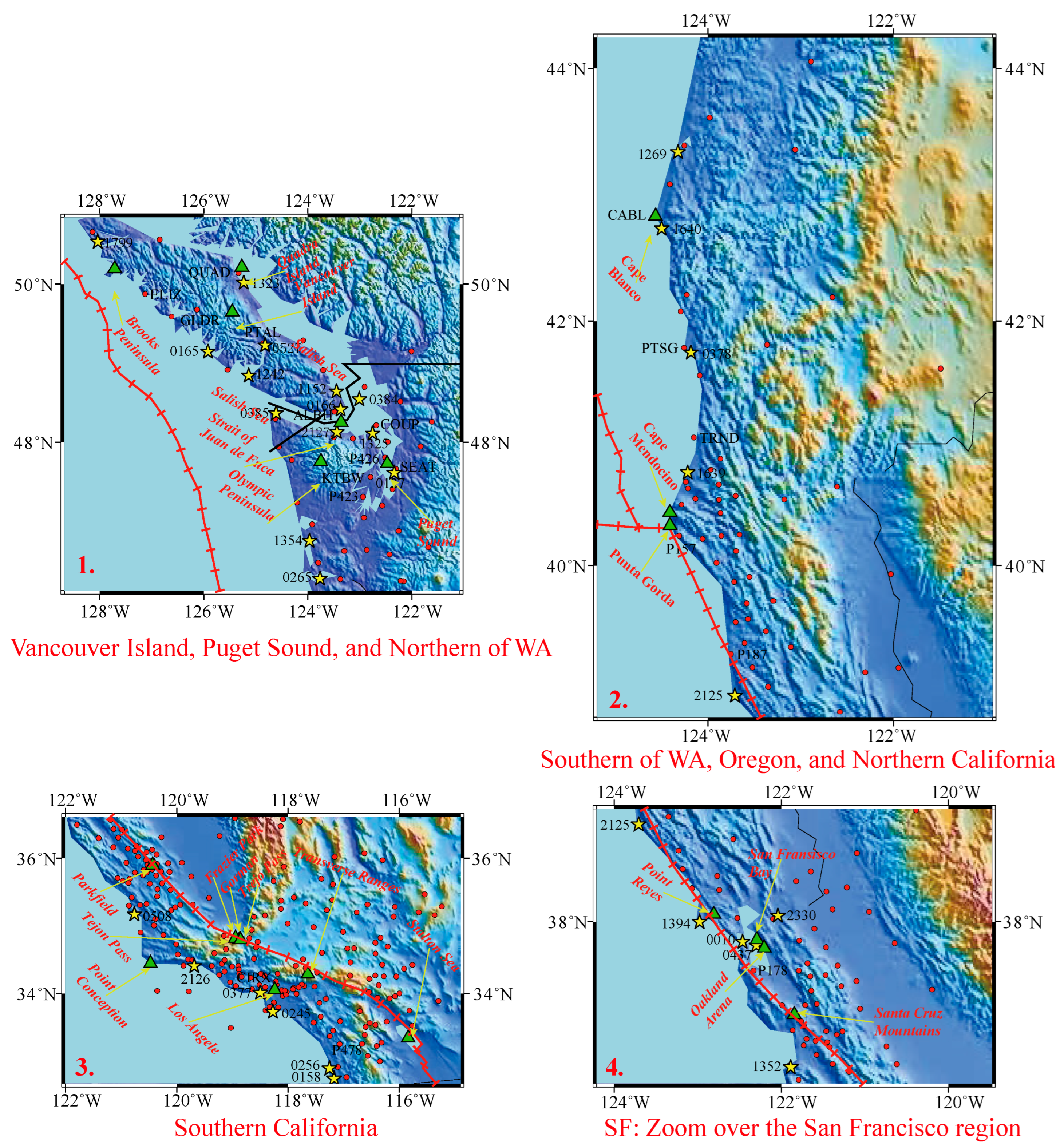
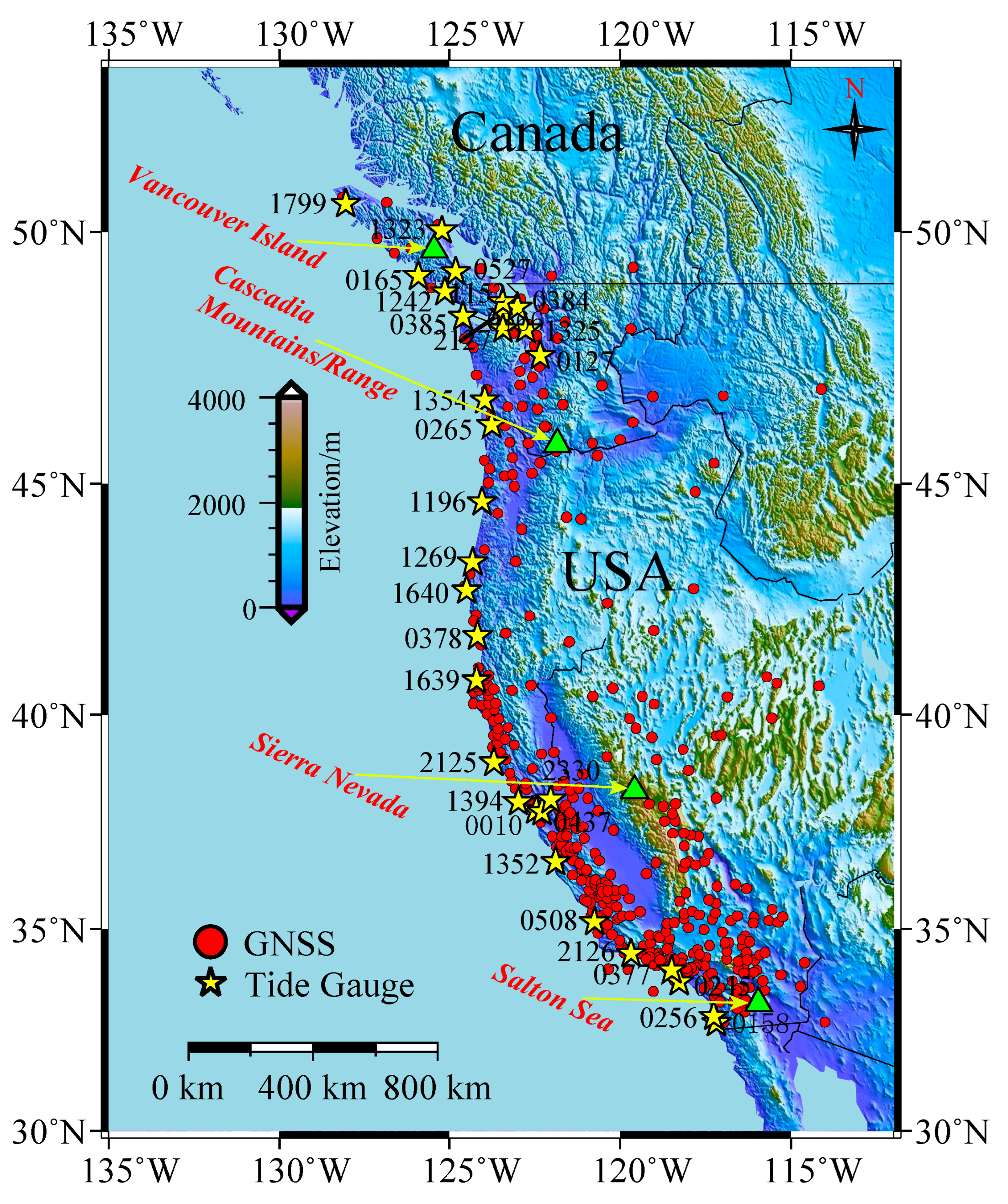
3.1. Overview of the Tectonics of the Pacific Coast and Coastal Uplift Profile

Broadly speaking, the Pacific coast is divided by two different geodynamic areas: the Pacific Northwest and the center to Southern California. The Pacific Northwest down to the triple junction at Cape Mendocino is a subduction zone defined by the Cascadia mountains where the Pacific plate subducts under the North American plate. It is a very long, sloping subduction zone where the Explorer, Juan de Fuca, and Gorda plates move to the east and slide below the much larger mostly continental North American Plate [67]. The triple junction is the location of a change in the broad plate motions which dominate the west coast of North America, linking convergence of the northern Cascadia subduction zone and translation of the southern San Andreas fault system. The fault passes along the towns of Gorman, Tejon Pass, and Frazier Park, and begins to bend northward, forming the “Big Bend”. This restraining bend is thought to be where the fault locks up in Southern California. The southern segment, which stretches from Parkfield in Monterey County all the way to the Salton Sea, and 56.0 km close to the northeast of Los Angeles, can generate large earthquakes (wit moment magnitude > 8.0). The fault is a right-lateral strike-slip with various degrees of compression forces. Along the fault, the locking zone varies due to the geodynamic complexity created from:
(1) The network of faults running parallel to the San Andreas fault in Northern and Central California.
(2) The change of geometry (e.g., upturned around the Salton Sea area).
(3) The various degrees of compressional forces between the Northern American plate towards the Pacific Plate, forcing the San Andreas fault to jog westward. The complexity of this fault system, which includes the sister faults (e.g., Rodgers Creek Fault, Hayward Fault, Calaveras Fault) can be witnessed by the creation of various mountain ranges along the fault, e.g., the Transverse Ranges in Southern California and Santa Cruz Mountains [68,69,70].

3.2. Vancouver Island, the Olympic Peninsula, and Puget Sound

Previous studies [1,24,71] show that the Cascadia fore arc is divided in three areas. The Cascadia subduction zone generates a large uplift rate observed on the northern part of Vancouver Island and the Olympic peninsula with an order of magnitude 2.0 mm/yr on average, resulting from the combination of the postglacial rebound and the subduction interseismic strain, Figure 4 supports previous results, where the VLM values around Vancouver island are gradually increasing from the Olympic peninsula (1.40 mm/yr) reaching around 2.3 mm/yr on average (see green line in Figure 4), and large uplift at the north of the island (e.g., Quadra island-QUAD 4.2 ± 0.5 mm/yr (PANGA); 3.5 ± 0.2 mm/yr (NMT), Port Alberni (PTAL) 3.5 ± 0.3 mm/yr (PANGA), 2.5 ± 0.1 mm/yr (NMT)). We can underline that there is a discrepancy between our results and Montillet et al., 2018 at some stations. For example, ELIZ experiences a 2.8 ± 0.2 mm/yr (PANGA) whereas in the previous study it was reported an uplift of 2.5 ± 0.2 mm/yr. In addition, we estimate for KTBW with an uplift of −0.1 ± 0.3 mm/yr (PANGA), whereas in the previous study the estimate was about −0.1 ± 0.2 mm/yr. These discrepancies are due to the specific modelling of the geophysical signals (i.e., considering the ETS) and the optimum stochastic noise model selection.
On the opposite, the inland waterways and Puget Sound have a uniform small amplitude, with some places with negative values generated by an oblique fault with shallow fault systems in the central Puget Sound lowland [72,73]. Overall, Figure 4 supports previous studies [1,24]. Inland Puget sound is characterized by small positive or negative VLM values but with associated large uncertainties, e.g., SEAT at 0.5 ± 0.7 mm/yr (PANGA), −1.4 ± 0.8 mm/yr (NMT); P423 −0.2 ± 0.4 mm/yr (PANGA); −0.8 ± 0.2 mm/yr (NMT)). Thus, the new profile confirms the large variability of VLM estimates in the Pacific Northwest around the Cascadia subduction zone in agreement with previous studies [1,24]. Looking at Table A1 (in the Appendix A), some stations are experiencing large discrepancies with previous studies, namely Montillet et al., (2018) and Mazzotti et al., (2007) as discussed above for the uplift on Vancouver Island. Many of the Cascadia slow slip events are affecting the time series for the stations west of the Cascades range, and are hard to model away without a full slip model for each event, knowing that GNSS stations installed in the late 1990s may have recorded more than hundreds of them [70]. Our approach is based on estimating all the slow slip events together with a stochastic noise model selected using different information criterions (Ics, e.g., AIC/BIC/BIC_tp) [34]. Therefore, the parameter estimation suffers from under-/overestimation depending on factors such as the stochastic noise characteristics of the data and the type of estimator used [40,41]. In our case, we are using the maximum likelihood estimator [36].
Looking at the differences between the various Ics in Table A2 (see Appendix A), the stochastic properties of VLM estimates do not vary for about 98.0% of the stations for both the PANGA and NMT solutions. This is due to the low percentage of stochastic noise model change. Table A2 (in the Appendix A) shows the difference in model selection for each station and for both the PANGA and NMT of the analyzed GNSS stations. The results show that the difference of the AIC, BIC, and BIC_tp selection is marginal for most of the sites, with only a few sites displaying a significant difference. Therefore, only the BIC_tp is used to select the optimal stochastic noise model in the following analysis.
Table 2 shows that the PL+WN model still appears to be the best noise model, accounting for 81.0% and 61.0% of the PANGA and NMT solutions, and the GGM+WN accounts for 14.0% and 34.0%, respectively, consistent with He et al. [40,41]. Besides, we made a statistical analysis of the ratio of velocity and velocity uncertainty with the selected optimal noise model for the PANGA and NMT solutions. The NMT is noisier than the PANGA solution when we estimate the ratio between velocity and velocity uncertainty (cf. Table 3).

3.3. South of Washington State and Oregon

Figure 3 shows that VLM decreases towards the south of Washington State (WA), reaching almost zero at the top and central parts of Oregon (Coos Bay). The VLM estimates are below 1 mm/yr (at P396 0.8 ± 0.2 mm/yr (BIC_tp–PANGA), −0.2 ± 0.4 mm/yr (BIC_tp–NMT)); at CHZZ −0.2 ± 0.3 mm/yr (PANGA), and −0.8 ± 0.4 mm/yr (NMT–BIC_tp)). This result is further emphasized by looking at the mean of the VLM (green line) which is around 0.0 mm/yr between central Oregon (plains) and the south of Washington state.
Figure 5 compares the mean and variance region-by-region where all the 405 stations processed are used. We can observe that the two solutions are comparable in terms of variance for all regions of the Pacific coast. However, there is an offset in terms of mean value ≈±1.2 mm/yr depending on the selected region. For example, for the Oregon–Southern Washington region, the mean is centered at 0.0 for the PANGA solution and ≈−1.2 mm/yr for the NMT solution. This result underlines the difference in the strategy of these two processing centers.

3.4. Cape Blanco–Cape Mendocino and Point Arena in Northern California

Towards the south of Oregon, at Cape Blanco and down to Cape Mendocino, the VLM increases progressively (CABL 1.5 ± 0.1 mm/yr (PANGA); 0.8 ± 0.2 mm/yr (NMT)) to reach more than 2mm/yr for the PANGA solution at PTSG 2.87 ± 0.34 mm/yr, and ≈2.0 ± 0.5 mm/yr for the NMT product. However, the uplift estimated from the NMT solution increases up to 1.4 ± 0.3 mm/yr when not estimating any post-seismic relaxation or transient signal (just co-seismic offsets). These uplift increases are due to the geophysical/geodynamic activities at the Mendocino triple junction, where the Cascadia interseismic strain accumulation locks the subducting Gorda slab underneath the North American plate [74].
Figure 6 also shows that the VLM coastal profile between Cape Blanco and south of Cape Mendocino (Northern California) is not smooth with drops (at TRND −1.0 ± 0.6 mm/yr (PANGA); −1.2 ± 0.9 mm/yr (NMT)). This instability is due to the numerous co-seismic offsets and geophysical signals necessary for estimation caused by the intense geodynamic activity in this particular area. The San Andreas fault originates offshore from the triple junction bending to follow the Northern California coastline underwater up to Point Arena, then with various on- and offshore areas (e.g., Point Reyes), and continues completely inland along Southern California from south of the San Francisco Bay [75]. We can observe in Figure 6 that the uplift is not large when the fault is offshore (e.g., near Punta Gorda at P157 0.5 ± 0.4 (PANGA) and 0.6 ± 0.5 mm/yr (NMT)), whereas the uplift is larger when the fault is onshore (at Point Arena—P187 3.3 ± 0.8 mm/yr (PANGA); 2.8 ± 0.6 mm/yr (NMT)). Therefore, the non-smoothness of the coastal VLM profile translates into the intense geophysical activity intrinsic to this area. Looking at Figure 5, the PANGA uplift estimates in this region are on average close to zero mm/yr, but with a standard deviation of 2.0 mm/yr, which is twice the standard deviation of the southern Washington and Central Oregon area. Note that the NMT values are similar, with a slightly smaller mean value (≈−0.5 mm/yr).

3.5. Central and Southern California

The southern San Andreas Fault system is onshore passed San Francisco Bay. The center section runs near Parkfield and Hollister, experiencing a phenomenon called aseismic creep [76,77], where the fault slips continuously without causing any earthquakes. However, the southern part, running through Parkfield, has experienced several large earthquakes, e.g., the 1989 Loma Prieta earthquake with a moment magnitude of 6.9 [78]. The southern segment is generally defined as the part of the fault running from Parkfield in Monterey County to Bombay Beach on the border of the Salton Sea, passing through the base of the San Gabriel and San Bernardino mountains. These mountain ranges are the testimony of San Andreas fault activity [79].
Figure 6 shows that the coastal VLM profile decreases from Point Arena to a minimum at the south of the San Francisco Bay (P178: −2.1 ± 0.4 mm/yr, PANGA), however, the NMT product provides an estimate of the same order of magnitude (i.e., −2.7 ± 0.6 (NMT)) of P187 (Point Arena). This shows the difficulty of estimating reliably the VLM closest to an active fault where the two strategies have a noticeable impact on the uplift estimates. However, the VLM profile decreases further from the fault and from the shoreline. For example, after Point Reyes and the back of L.A., at the CIRX station we estimate 0.7 ± 0.3 mm/yr (PANGA) and −0.2 ± 0.5 mm/yr (NMT). Towards the south of L.A. and San Diego the VLM decreases (P478 −1.5 ± 0.4 mm/yr (NMT); −0.6 ± 0.3 mm/yr PANGA). In Figure 5 the scatter of the uplift estimates for the whole Southern California region is ≈3.0 mm/yr, bigger than for Vancouver Island and the Olympic Peninsula and slightly smaller than in the Inland Puget Sound area for the PANGA values. On average, the NMT product for the whole Southern California region provides comparable values estimated for Vancouver Island and the Olympic Peninsula combined together. The homogeneity of the VLM coastal profile is difficult to realize in Southern California due to the nature of the San Andreas Fault (right-lateral strike-slip) with various degrees of compression along the fault, compared with the Cascadia subduction mechanism and the VLM pattern in the Pacific Northwest [80]. However, we can notice that Southern California and the Inland Puget Sound are two areas with a complex geophysical mechanism, therefore generating a non-smooth VLM coastal profile [81].
Finally, Figure 7 displays the linearly interpolated uncertainties of the VLM around the whole west coast for both the PANGA and NMT products. It clearly shows the active geodynamic areas along the Pacific coast which agree with the VLM coastal profile derived in Figure 4 and Figure 6. For example, the subduction zone in Inland Puget Sound (WA) produces large uncertainties, together with the activity linked to the triple junction in Northern California. One can also underline the difference between the two solutions, where the large uncertainties seem to decrease in amplitude when the San Andreas fault comes onshore for the PANGA estimates, but it extends further south with the NMT solution. Moreover, the NMT product shows more smoothness around geodynamic active regions (Vancouver Island + Puget Sound, Southern California).

4. Discussion

4.1. RSLR and ASLR Estimation along the Pacific Coast

We estimate the RSLR [82] using 31 TGs located along the Pacific coast between 32°N and 51°N (see Figure 1 and Figure 8, Table 1 and Table A3 together with RSLR using SSH product). To recall Section 2, the same methodology is used to select the stochastic noise model with the ICs when estimating the relative SLR, and to a certain extent the mean sea level with the SSH product. Negative RSLR values are located in the Pacific Northwest—Vancouver Island and Olympic Peninsula—at stations such as Campbell River (CAMP) (−1.8 ± 0.4 mm/yr) and Neah Bay (Ne.B) (−1.8 ± 0.1 mm/yr). The average over the whole of Vancouver Island is −1.0 ± 0. 6 mm/yr. Two factors are here biasing these values: (i) the large uplift estimated from the GNSS time series due to the geodynamics of the Cascadia subduction zone; (ii) the GIA activity [24,63]. For the Puget Sound area, the mean RSLR value is around 1.3 ± 0.3 mm/yr. For example, at the TG of Seat, the value is ≈2.1 ± 0.1 mm/yr (see Table A3). Towards the south of Washington and the center of Oregon, the RSLR values are on average 1.1 ± 0.8 mm/yr, except at Astoria (ASTO) (−0.2 ± 0.2 mm/yr) due to the location of the TG inside the estuary of the Columbia River as discussed in [1,24,81].
Towards the triple junction, the RSLR decreases abruptly at Crescent (CRES see Table 1 and Figure 1) (−0.8 ± 0.2 mm/yr) and increases at its maximum along the whole Pacific coast at Humboldt Bay (HUMB) (5.7 ± 0.9 mm/yr) which is located near Cape Mendocino. From Humboldt Bay to Southern California, the RSLR values are large, with an average of 1.8 ± 0.4 mm/yr (La Jolla—LaJo). The large increase at Humboldt is probably due to a combination of various factors. First, the TG is located relatively near the triple junction tectonic activity, where the VLM is negative (P162 −1.6 ± 0.8 mm/yr PANGA) which may be the result of the tectonic activity. Secondly, we cannot discard the effect of ocean eddies on TG measurements due to the geophysical location of this TG. The authors in [83] have discussed the potential bias due to strong ocean eddies on the estimation of mean sea level rise. Central and Southern California show a large RSLR, which can be associated with a high risk of flooding in coastal areas and cities as discussed in NRC (2014) and in [82,84].
Note that in terms of comparing the differences of RSLR estimates between the stochastic noise models, we can only observe a marginal difference, especially between the GGM and ARMA models with a level of difference below 0.1 mm/yr on average, i.e., nothing significant. The ARFIMA can generate much larger uncertainties such as Port Chicago, CA (P. Ch. see Table 1) with a RSLR ≈2.4 ± 1.3 mm/yr compared with the GGM estimate of ≈2.0 ± 0.9 mm/yr and the ARMA estimate ≈2.0 ± 0.8 mm/yr. One may also observe similar results between the three ICs, especially BIC and BICtp. The RSLR estimates with the BIC_tp, can vary slightly. For example, at Patricia Bay (P.Ba), the RSLR is ≈0.4 ± 0.2 mm/yr (ARFIMA–BIC_tp) and ≈1.1 ± 1.1 mm/yr (ARFIMA–BIC and BIC_tp).

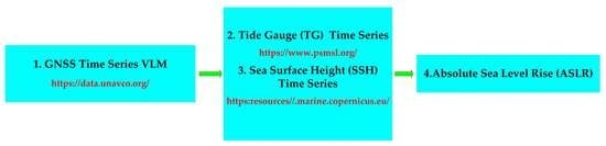
4.2. Absolute SLR along the Pacific Coast of the USA Using SSH and Corrected TG Measurements

We correct the RSLR with VLM interpolated from our coastal profile in order to estimate the ASLR [85]. Figure 9 displays the RSLR (BIC_tp), ASLR (BIC_tp), glacial isostatic adjustment (GIA, ensemble of models from NRC 2015), and the risk of coastal flooding (see line center on 0 mm/yr). The results displayed are only for the PANGA solution, but the associated values for both the PANGA and NMT are listed in Appendix A (see Table A4 and Table A5). To simplify this study, we select here only the BIC_tp criterion (for there are not many differences between the ICs for the VLM and the RSLR. However, AIC and BIC have known biases, which is why He et al., 2019 and 2021 [40,41] have shown that BIC_tp is more reliable) in the optimal noise model selection in order to estimate the VLM profile used in the interpolation at each TG. This simplification is based on the results in Section 3 where we expose the marginal differences between the criterions. In addition, we have only chosen the GGM model following our previous results on the RSLR. The GIA model (gray line) is produced by an ensemble of models provided by the previous study by the NRC (2014). In addition, the indices of flooding are provided by the work of [86].
Figure 10 clearly shows that when using the PANGA product the average ASLR for the Pacific Northwest (Vancouver Island and Puget Sound) is ≈3.0 mm/yr (PANGA–GGM), whereas the value is shifted to ≈1.2 mm/yr in Central and Southern California. Compared with the NMT product, the mean ASLR values between the Pacific Northwest and Central/Southern California are ≈3.1 mm/yr and ≈0.8 mm/yr, respectively. Therefore, we observe a much bigger variation (about 90.0–150.0%) after correcting from VLM the RSLR in the Pacific Northwest which is predominantly due to the GIA. The VLM correction to the RSLR accounts for both GIA and tectonic strain accumulation. Isolating the two sources of uplift is a difficult exercise that requires precise knowledge of mantle viscosity, recent glaciation history, and interseismic coupling of the faults around the coast [24]. It was shown by Montillet et al. [24] that this correction of the RSLR with VLM in the Pacific Northwest indicates that half of the VLM on Vancouver Island arises from GIA and the rest from the subduction-related strain. The GIA correction is much smaller in Central and Southern California. It is also observed that the estimates are close to the profile estimated from satellite altimetry, especially in the Los Angeles and San Diego areas for both the PANGA and NMT. Therefore, we can conclude that in this area, the geodynamics of the continent are not biasing the RSLR as much as in other places along the Pacific coast such as in the Pacific Northwest–Vancouver Island, Olympic Peninsula, and inland Puget Sound.
Moreover, we can compare the estimation of the SLR with either the SSH or the ASLR (cf. Figure 11 for the PANGA solution and Figure A2 for the NMT solution). Overall, the SLR estimates with SSH are all positive values across the entire coast. This result is expected because the satellite altimetry is not affected by the underlying geodynamical movements due to the vertical land motion affecting the TG measurements. Because satellite altimeters have a limited ability to measure sea level height in coastal regions where the TGs are installed, the SSH measurements are not affected by the VLM [87].
The second result is the general trend. The velocity uncertainty estimated with the SSH are small, on average 1.3 ± 0.2 mm/yr (ARMA), compared with the ASLR derived from the TG with a value to 1.3 ± 0.3 mm/yr (ARMA–PANGA) or 0.5 ± 0.4 mm/yr (ARMA–NMT). In the areas with underlying complex geodynamics, we have a greater SLR. The SLR shows a large average value of 2.9 ± 1.1 mm/yr, whereas the ASLR (TG+VLM) is around 2.0 ± 1.3 mm/yr (ARMA–PANGA). In Southern California, starting at Point Reyes, we have a steady increase with an average SSH of 1.4+/1.7 mm/yr. The ASLR estimated in the same region is around 1.6 ± 1.3 mm/yr (PANGA–ARMA) or 0.8 ± 1.1 mm/yr (NMT–ARMA). Overall, the SSH and ASLR products are generally comparable, especially with the PANGA solution. Furthermore, one factor generating the differences between the two products is the ocean eddies, which have been known to impact the monitoring of SLR [83]. Several methods have been developed that mix the TG and SSH products [88], but there is no consensus on how to reconcile both the TG and SSH measurements due to many underlying geodynamical phenomena intrinsic to each product.
Finally, twentieth-century rates for the Western Pacific are more similar to twenty-first-century global rates of 3.2 ([2.8–3.6]) mm/yr [89], whereas the Eastern Pacific satellite rates are significantly lower than the global mean value. However, twentieth-century satellite geocentric ocean height rates show a global mean of 1.5 to 1.9 mm/yr, or roughly half that of twenty-first-century rates (IPCC, 2013). We estimate the mean SLR over the whole Pacific coast as shown in Table 4.
Table 4 shows that the uncertainties of the ASLR using the NMT product to estimate the VLM are much higher than the ASLR value for all three models. The VLM estimates from the NMT product have been shown to differ substantially from the PANGA product. This result was already investigated in [24] where the analysis of the processing from the two centers reveals that this discrepancy is due to a processing strategy and how the scale from the Helmert transformation is handled as discussed in Section 2.1. This issue was also highlighted in [41] when comparing both processing strategies (PANGA, NMT) and emphasizing the largest variations for the NMT product in the estimated tectonic rates and vertical land motion values from an analysis of hundreds of GNSS stations located in North America. Furthermore, we have used stations from the whole Pacific coast which includes two regions with high tectonic activity (i.e., the Cascadia subduction zone and the San Andreas fault). Even though we have carefully modeled each GNSS time series, multidecade transients will impact rate estimates differently based on both the time series duration and the structure of any known long-term transients. Compared with several studies, e.g., [24], we have here used criteria to optimally select the stochastic noise models. Our analysis emphasizes that the GNSS product [e.g., PANGA, NMT] should be carefully chosen when estimating the ASLR. The second result from the analysis of Table 4 is that the ARFIMA model tends to produce larger uncertainties. This result should be further investigated in the next study.
Finally, our estimates with the PANGA and SSH are within [1.5–1.9] mm/yr. There is an ongoing discussion in the scientific community about the discrepancy between the GMSL and the ocean height which focuses on the estimation of the acceleration in sea level rise rates (IPCC, 2013). However, this topic was left for a future study.

5. Conclusions

This paper investigates the selection of the stochastic noise models of geodetic time series (i.e., GNSS daily position, TG, and SSH) and the estimation of sea level rise on the Pacific coast from Vancouver Island (CA) to Southern California (USA). First, we analyze the stochastic noise properties of 405 permanent GNSS stations distributed over the west coast of the USA using the NMT and PANGA products. The selection of the optimum stochastic noise (i.e., FN+WN, RW+FN+WN, GGM+WN, and PL+WN) model is based on the ICs (i.e., AIC/BIC/BIC_tp). The crustal uplift is estimated by a joint inversion of functional (i.e., geophysical signals) and stochastic noise models. We then provide a coastal profile for the VLM.
Secondly, we estimate the RSLR from 31 century-long TG records. The estimates are then corrected with the VLM interpolated at each TG location from our coastal profile in order to obtain the ASLR. Besides, for comparison with our ASLR estimates, we use the SSH product estimated at the location of each TG modulo the resolution of the selected satellite altimetry product (with grid data with a data resolution of 5′).
The following conclusions are drawn from our study:
(1)
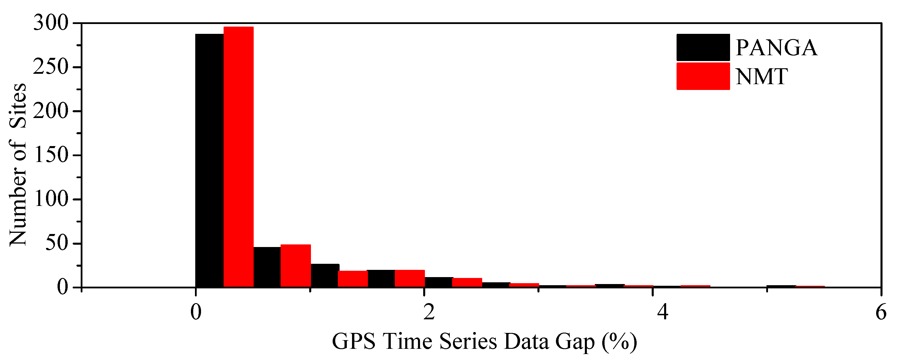
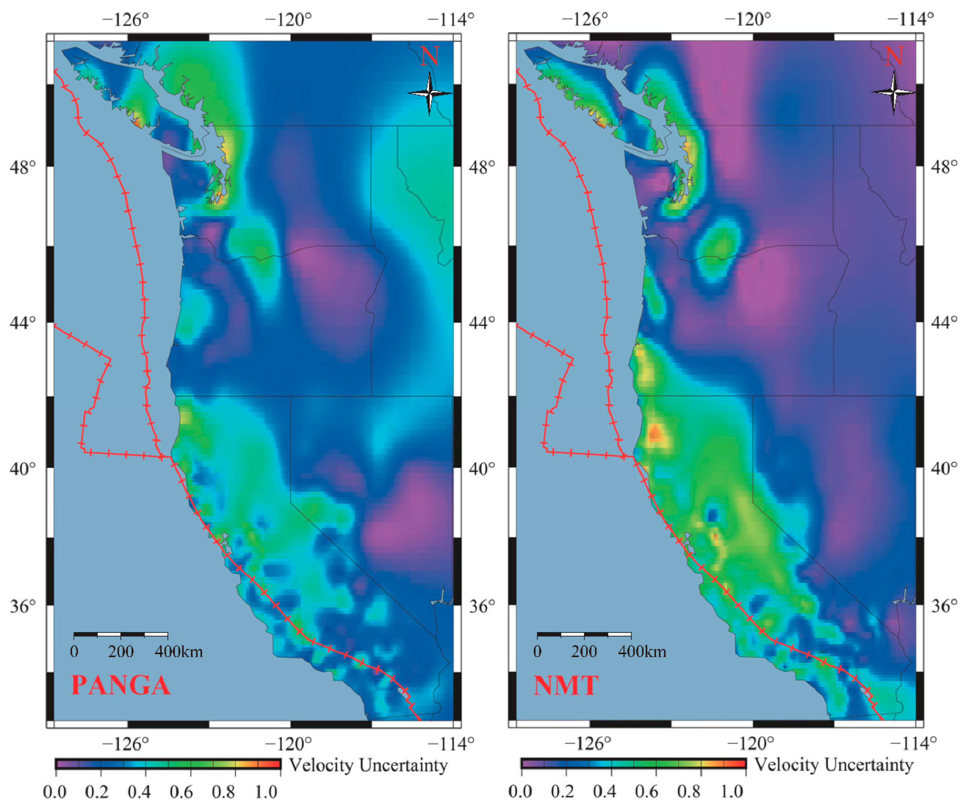
For the 405 analyzed GNSS daily position time series, the PL+WN model still appears to be the best noise model, i.e., about 81.0% and 61.0% of the PANGA and NMT solutions. The GGM+WN accounts for about 14.0% and 34.0% of the PANGA and NMT, respectively. Overall, the values for the NMT product are noisier than the PANGA solution, which is consistent with [40,41]. Besides, the stochastic properties of VLM estimates are not varying using the various ICs for about 98.0% of the stations for both the PANGA and NMT solutions.
(2)
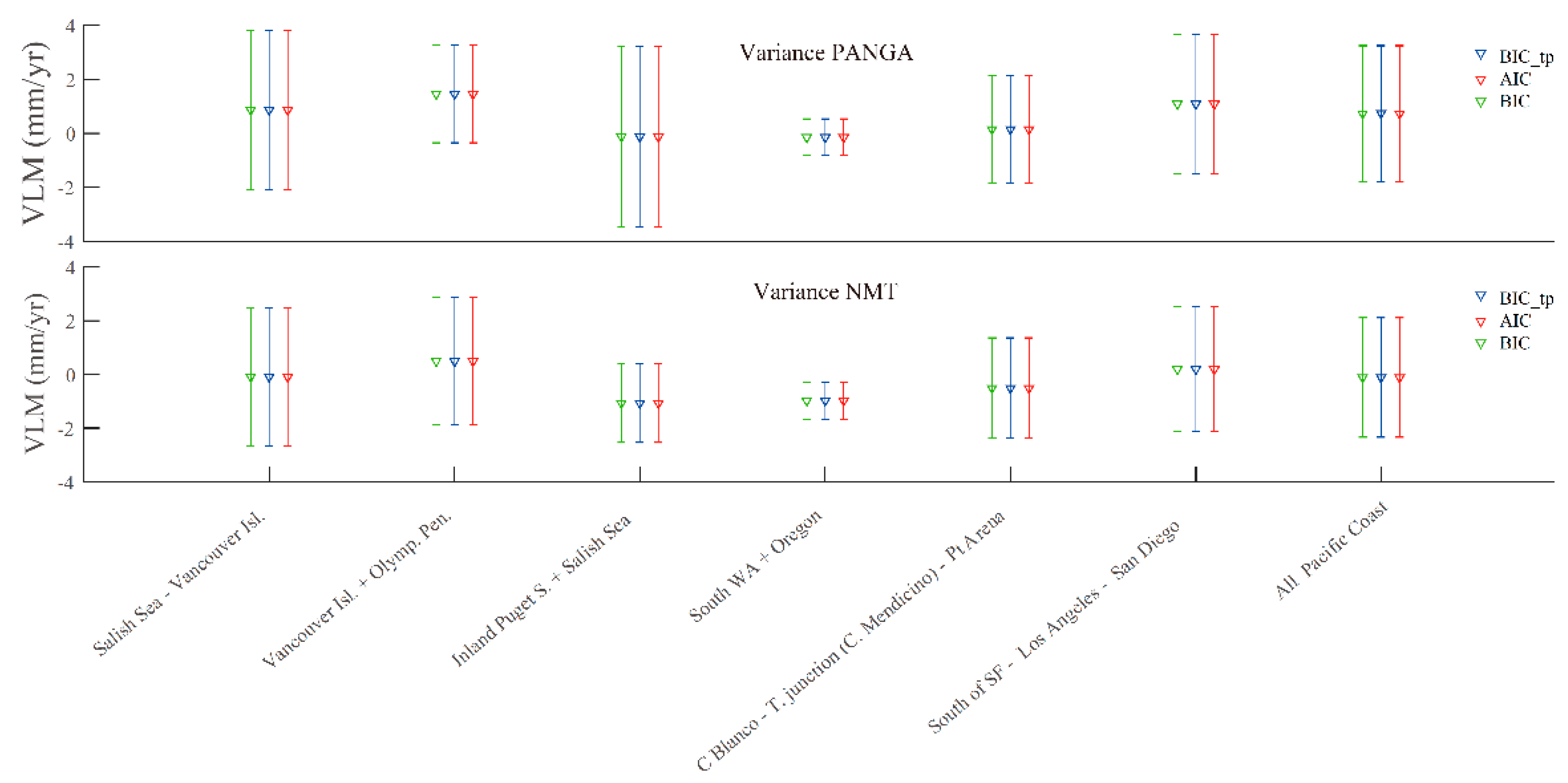
The Cascadia forearc is divided into three areas: Vancouver Island, the Olympic Peninsula, and Puget Sound, among them the Cascadia subduction zone generates a large uplift rate observed on the northern part of Vancouver Island and the Olympic Peninsula with an order of magnitude about 2.0 mm/yr on average, which is caused by the combination of the postglacial rebound and the subduction interseismic strain, whereas the inland Puget Sound is characterized by small positive or negative values VLM values. This result supports previous studies (e.g., Mazzotti et al., 2007; Montillet et al., 2018) that the VLM values around Vancouver Island are gradually increasing from the Olympic Peninsula [1,24]. We also underline that some stations do not experience as much uplift as reported in the previous work of Montillet et al., (2018) [24]. These discrepancies are due to the specific modeling of the geophysical signals (e.g., the ETS events) and the optimum stochastic noise model selection. In addition, the new profile confirms the large variability of VLM estimates in the Pacific Northwest around the Cascadia subduction zone in agreement with previous studies.
(3)
The VLM decreases towards the south of WA and the Oregon region. We also conclude that the PANGA and NMT processing are comparable in terms of variance for all regions of the Pacific coast. From Cape Blanco down to Cape Mendocino the VLM increases progressively, which is due to the geophysical activities at the Mendocino triple junction. For Central and Southern California, the NMT product for the whole Southern California region provides comparable values estimated for Vancouver Island and the Olympic Peninsula combined.
(4)
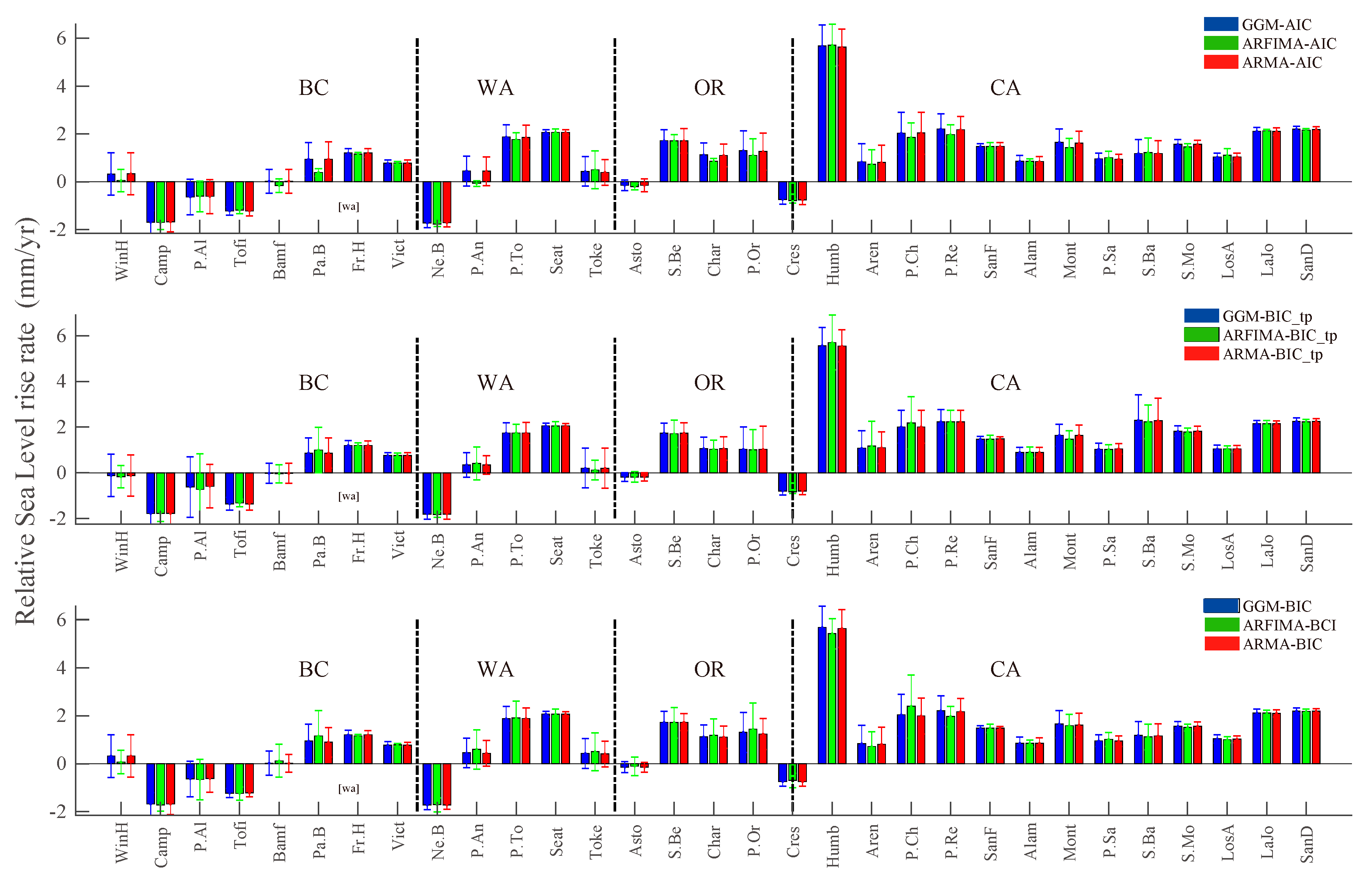
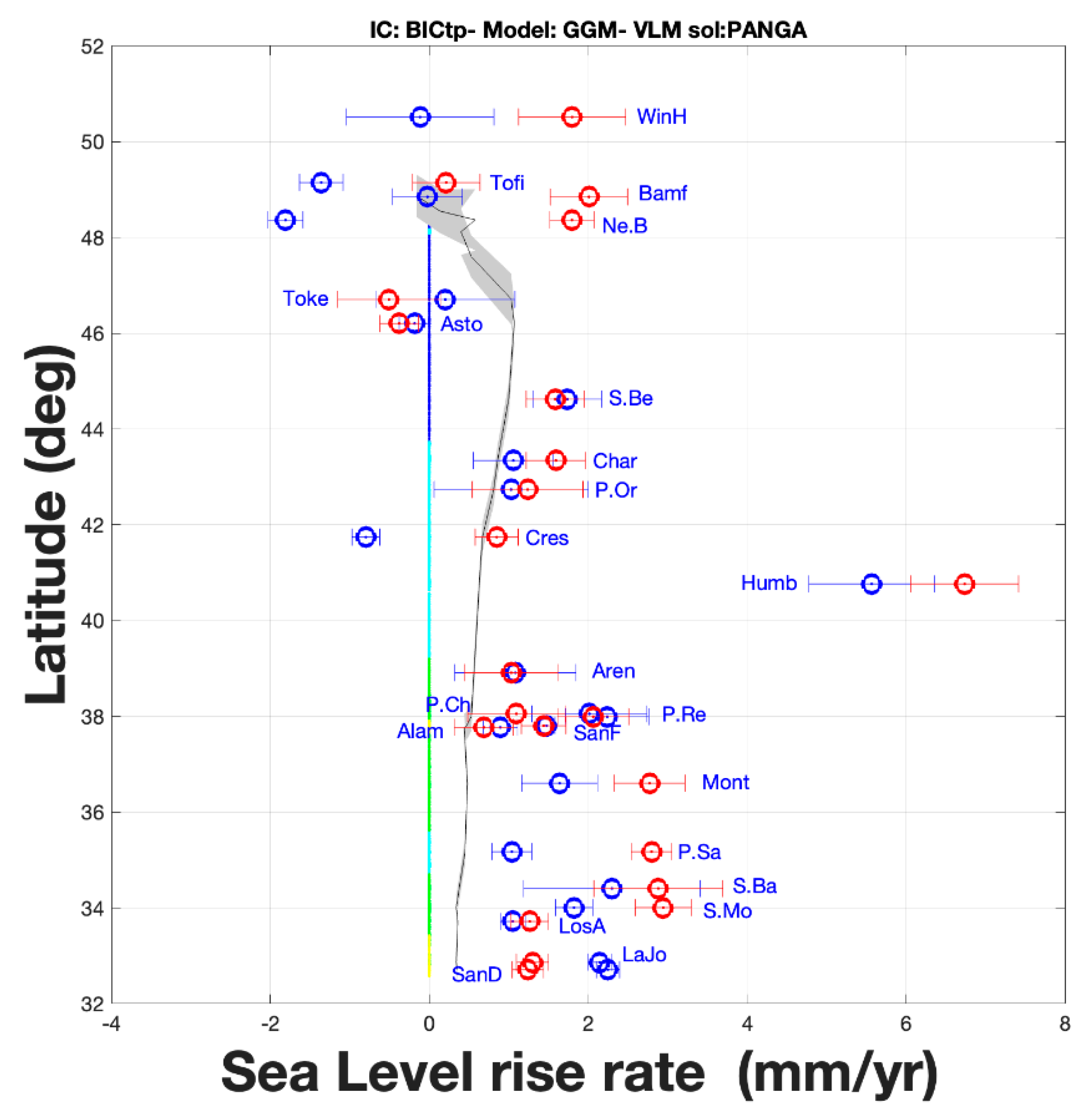
We estimate the RSLR and ASLR along the Pacific coast. The negative RSLR values are mostly located in the Pacific Northwest—Vancouver Island and the Olympic Peninsula—with stations such as Campbell River (Camp).
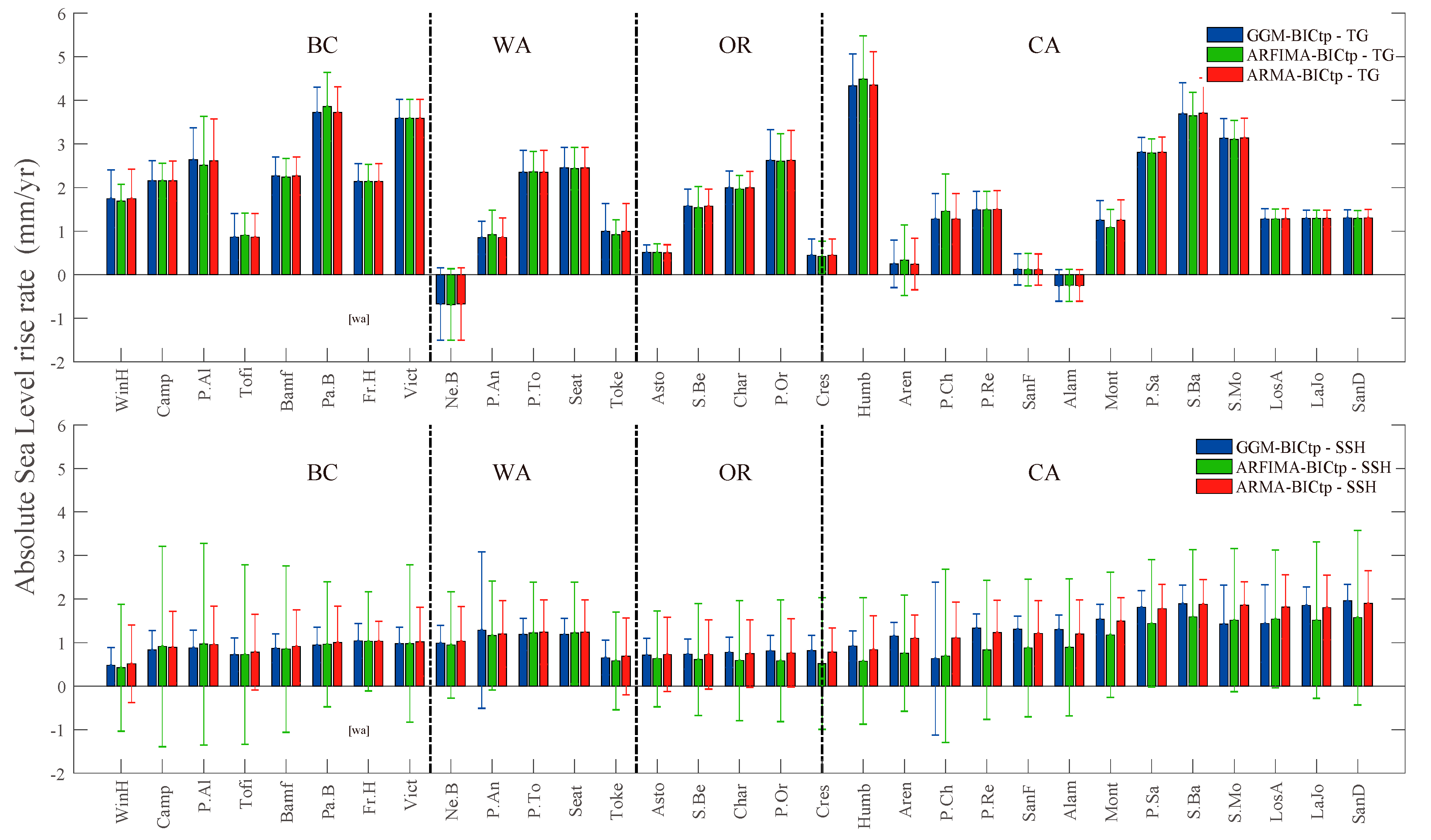
(5)
We observe a much bigger variation (about 90.0–150.0%) of the ASLR in the Pacific Northwest which is predominantly due to the GIA. Moreover, we compared the estimation of the ASLR with the SSH. The SLR estimated with the SSH product are all positive values across the entire coast. This result is expected because the satellite altimetry is not affected by the underlying geodynamical movements due to the VLM affecting the TG measurements. They are comparable for the center of the coast (Southern WA, Oregon planes, and some parts of Southern California) where the tectonic activity does not influence the TG measurements. However, the discrepancy between the SLR and the SSH is still discussed within the scientific community due to many factors such as the underlying geodynamics and ocean eddies. Our analysis also emphasizes the need to carefully chose the GNSS product that can introduce different variations of the VLM and then influences the estimated ASLR.
(6)
Finally, we compare our various estimates with the twentieth-century satellite geocentric ocean height rates, which are between 1.5 and 1.9 mm/yr. Our estimates with the PANGA and SSH are consistent with the previous studies.
As Hammarklint [89] pointed out, global ocean levels have always fluctuated with changes in our climate. The underlying factors causing sea level change and the relationship between sea level change and climate need to be further studied.

Author Contributions

X.H. and J.-P.M., writing—original draft preparation; R.F., T.I.M. and W.J., methodology, review and editing; Z.H. and X.H., data processing and figure plotting. All authors have read and agreed to the published version of the manuscript.

Funding

This work was sponsored by National Natural Science Foundation of China (42104023), Jiangxi University of Science and Technology High-level Talent Research Startup Project (205200100564, 205200100588), Youth Talent Plan of the Science and Technology Think Tank of China Association for Science and Technology in 2022 (No.207), 2021 Jiangxi Province Higher Education Teaching Reform Research Project (JXJG-21-7-37), and Jiangxi Provincial Natural Science Foundation (20212BAB204030).

Data Availability Statement

The data for both the PANGA and NMT processing centers are available freely at https://data.unavco.org/ (cwu.final_nam08.pos.tar and nmt.final_nam08.pos.tar) (acceesed on 10 January 2022). The TG measurements are available at https://www.psmsl.org/ (acceesed on 10 January 2022). The SSH product is downloaded from https://resources.marine.copernicus.eu/ (acceesed on 10 January 2022).

Conflicts of Interest

The authors declare no conflict of interest.

Appendix A

Table A1. Comparing the velocity (u) and uncertainty (sigma) with previous studies of Montillet et al. (2018) and Mazzotti et al. (2007).
SiteThis WorkMontillet et al. 2018 [24]Mazzotti et al. 2007 [1]
PANGANMTPANGANMT
uSigmauSigmauSigmauSigmauSigma
ALBH1.20.10.30.10.70.20.80.31.10.9
DRAO0.40.2−0.10.21.00.21.20.31.20.7
NANO1.70.51.70.62.20.31.80.42.50.9
NEAH3.40.12.20.13.20.23.20.33.51.0
PGC51.00.20.40.10.80.20.10.51.81.0
SEAT0.50.7−1.40.80.10.3−0.20.3−0.60.9
UCLU1.81.0−0.71.12.50.21.90.32.70.9
BAMF2.10. 41.90.82.70.41.80.4
BCOV2.70.21.80.32.80.23.60.7
CABL1.50.10.80.21.20.21.40.2
CHZZ−0.20.3−0.80.40.20.40.80.2
ELIZ2.80.21.70.12.50.22.60.4
HOLB1.90.21.30.22.40.20.91.0
KTBW−0.10.3−1.00.5−0.50.2−0.40.3
NTKA2.70.22.00.33.60.24.30.4
P159−1.20.4−1.70.6−0.80.3−1.60.3
P161−1.50.5−2.10.8−1.00.2−1.50.3
P162−1.60.8−2.20.7−1.20.2−1.60.3
P316−2.10.8−2.30.7−2.20.5−2.10.6
P3622.00.31.60.32.80.32.10.4
P3641.90.21.20.22.30.31.70.4
P3650.50.2−0.10.21.00.30.00.4
P3660.40.2−0.70.20.70.3−0.60.3
P367−0.30.3−1.10.2−0.20.3−0.80.4
P3950.60.40.20.70.20.4−0.20.3
P3960.80.2−0.20.41.10.50.20.4
P3980.70.4−0.10.11.50.30.60.4
P4022.10.21.40.22.50.21.70.5
P423−0.20.4−0.80.2−0.40.2−0.90.3
P435−0.20.3−0.60.30.60.40.10.4
P4370.60.8−1.40.8−0.40.3−1.40.7
P4391.00.6−0.60.70.00.2−0.30.4
P7342.40.41.70.53.20.32.00.4
PABH0.50.2−0.30.10.20.20.20.3
PCOL−0.00.9−2.40.9−0.60.3−0.60.3
PTAL3.50.32.50.13.50.10.00.6
PTSG2.90.32.00.53.60.23.00.3
QUAD4.20.53.50.24.30.43.90.4
SC041.40.20.70.31.20.21.00.2
TPW20.50.1−0.30.10.20.20.50.2
TRND−1.00.6−1.20.9−0.90.3−0.70.3
Table A2. Optimal noise model differences between the various ICs for the analyzed 405 GNSS sites.
SolutionSiteAICBICBIC_tp
PANGACHWKGGMWNPLWNPLWN
MIDAPLWNFNWNFNWN
P283PLWNFNWNFNWN
P315PLWNFNWNFNWN
P316PLWNFNWNFNWN
SHLDGGMWNPLWNPLWN
KTBWGGMWNPLWNPLWN
NMTP156PLWNFNWNFNWN
P178PLWNFNWNFNWN
P188PLWNFNWNFNWN
P267PLWNFNWNFNWN
P273PLWNFNWNFNWN
P312PLWNFNWNFNWN
PVRSPLWNFNWNFNWN
KTBWGGMWNPLWNPLWN
Table A3. Relative sea level rise (RSLR) derived from TG and SSH time series.
RSLR
TG
GGMARFIMA
BIC_tp
ARMA
BIC_tp
ARFIMA
BIC
ARMA
BIC
ARFIMA
AIC
ARMA
AIC
VelocitySigmaVelocitySigmaVelocitySigmaVelocitySigmaVelocitySigmaVelocitySigmaVelocitySigma
00101.50.11.50.21.50.11.50.21.50.11.50.21.50.1
01272.10.12.10.22.10.12.10.22.10.12.10.22.10.1
01582.30.22.20.12.30.12.20.12.30.12.20.12.30.1
0165−1.40.3−1.30.2−1.40.3−1.30.2−1.40.3−1.30.2−1.40.3
01660.80.10.80.10.80.10.80.10.80.10.80.10.80.1
02451.10.21.10.11.10.21.10.11.10.21.10.11.10.2
02562.20.22.10.12.10.12.10.12.10.12.10.12.10.1
0265−0.20.2−0.20.2−0.20.2−0.20.2−0.20.2−0.20.2−0.20.2
03771.80.21.80.21.80.21.80.21.80.21.80.21.80.2
0378−0.80.2−0.80.1−0.80.2−0.80.2−0.80.2−0.80.1−0.80.2
03841.20.21.20.11.20.21.20.11.20.21.20.11.20.2
0385−1.80.2−1.80.1−1.80.2−1.80.1−1.80.2−1.80.1−1.80.2
04370.90.20.90.20.90.20.90.20.90.20.90.20.90.2
05081.00.31.00.21.00.21.00.21.00.21.00.21.00.2
0527−0.61.3−0.71.6−0.61.0−0.71.6−0.61.0−0.71.6−0.61.0
11520.90.71.01.00.90.71.01.00.90.70.70.40.90.7
11961.70.41.70.61.70.51.70.61.70.51.80.31.70.5
12420.00.40.00.40.00.50.00.40.00.50.00.40.00.5
12691.10.51.00.41.10.51.00.41.10.51.00.41.10.5
1323−1.80.5−1.80.4−1.80.5−1.80.4−1.80.5−1.80.4−1.80.5
13251.80.51.80.41.70.51.80.41.70.51.80.41.70.5
13521.60.51.50.41.60.51.50.41.60.51.50.41.60.5
13540.20.90.10.40.20.90.10.40.20.90.10.40.20.9
13942.20.52.20.52.20.52.20.52.20.52.20.52.20.5
16395.60.85.71.25.60.75.71.25.60.75.71.25.60.7
16401.01.01.00.91.01.01.00.91.01.01.00.91.01.0
1799−0.10.9−0.20.5−0.10.9−0.20.5−0.10.9−0.20.4−0.11.0
21251.10.81.21.11.10.71.21.11.10.71.21.11.10.7
21262.31.12.20.72.31.02.20.72.31.02.20.72.31.0
21270.40.50.40.70.30.40.40.70.30.40.40.70.40.5
23302.00.72.21.12.00.72.21.12.00.72.21.12.00.7
RSLR
SSH
GGM
ARFIMA
BIC_tp
ARMA
BIC_tp
ARFIMA
BIC
ARMA
BIC
ARFIMA
AIC
ARMA
AIC
VelocitySigmaVelocitySigmaVelocitySigmaVelocitySigmaVelocitySigmaVelocitySigmaVelocitySigma
00101.30.30.91.61.20.80.91.61.20.80.91.71.20.8
01271.20.41.21.21.20.71.21.21.20.71.21.11.20.8
01582.00.41.62.01.90.71.62.01.90.71.61.91.90.7
01650.70.40.72.10.80.90.72.10.80.90.71.40.80.9
01661.00.41.01.81.00.81.01.81.00.81.01.61.00.8
02451.40.91.51.61.80.71.51.61.80.71.51.71.80.7
02561.90.41.51.81.80.71.51.81.80.71.51.81.80.7
02650.70.40.61.10.70.90.61.10.70.90.61.10.70.9
03771.40.91.51.71.90.51.51.71.90.61.51.71.90.6
03780.80.40.51.50.80.60.51.50.80.80.61.30.80.6
03841.00.41.01.11.00.51.01.11.00.51.01.21.10.7
03851.00.41.01.21.00.81.01.41.00.81.01.21.00.8
04371.30.30.91.61.20.80.91.61.20.80.91.61.20.8
05081.80.41.41.51.80.61.41.51.80.61.41.51.80.5
05270.90.41.02.31.00.91.02.31.00.90.91.41.00.9
11521.00.41.01.41.00.81.01.41.00.81.01.71.00.8
11960.70.30.61.30.70.80.61.30.70.80.61.30.70.8
12420.90.30.91.90.90.80.91.90.90.80.81.40.90.9
12690.80.40.61.40.80.80.61.40.80.80.61.40.80.8
13230.80.40.92.30.90.80.92.20.90.70.92.30.90.8
13251.20.41.21.21.20.71.21.21.20.71.21.11.20.8
13521.50.41.21.41.50.51.21.41.50.51.21.41.50.5
13540.70.40.61.10.70.90.61.10.70.90.61.20.70.9
13941.30.30.81.61.20.70.81.61.20.70.81.61.20.7
16390.90.30.61.50.80.80.61.50.80.80.61.50.80.8
16400.80.40.61.40.80.80.61.40.80.80.61.30.80.7
17990.50.40.41.50.50.90.41.50.50.90.41.50.50.9
21251.20.30.81.31.10.50.81.31.10.50.71.51.10.5
21261.90.41.61.51.90.61.61.51.90.61.61.51.90.6
21271.31.81.21.31.20.81.21.31.20.81.21.21.20.8
23300.61.80.72.01.10.80.72.01.10.80.81.61.10.8
Table A4. Absolute SLR estimation derived from PANGA.
TG
Site
GGMARFIMA
BIC_tp
ARMA
BIC_tp
VelocitySigmaVelocitySigmaVelocitySigma
00100.10.50.10.50.10.5
01272.50.72.40.72.50.7
01581.30.31.30.31.30.3
01650.90.80.90.70.90.8
01663.60.63.60.63.60.6
02451.30.31.30.31.30.3
02561.30.31.30.31.30.3
02650.50.30.50.30.50.3
03773.10.63.10.63.10.6
03780.40.50.40.40.40.5
03842.10.62.10.62.10.6
0385−0.71.2−0.71.2−0.71.2
0437−0.30.5−0.20.5−0.30.5
05082.80.52.80.52.80.5
05272.61.42.51.62.61.0
11523.70.83.91.13.70.8
11961.60.61.50.71.60.6
12422.30.62.20.62.30.6
12692.00.52.00.42.00.5
13232.20.72.20.62.20.7
13252.40.72.40.72.40.7
13521.30.71.10.61.30.6
13541.00.90.90.51.00.9
13941.50.61.50.61.50.6
16394.41.14.51.44.31.0
16402.61.02.60.92.61.0
17991.71.01.70.61.70.9
21250.20.80.31.10.30.8
21263.71.13.60.83.71.0
21270.90.60.90.80.80.5
23301.30.81.51.21.30.8
Table A5. Absolute SLR estimation derived from NMT.
TG SiteGGMARFIMA
BIC_tp
ARMA
BIC_tp
VelocitySigmaVelocitySigmaVelocitySigma
0010−0.60.7−0.60.7−0.60.7
01270.70.80.70.80.70.8
01580.40.40.40.40.40.4
0165−1.00.8−1.00.8−1.00.8
01661.40.71.40.71.40.7
02450.30.30.30.30.30.3
02560.40.40.40.40.40.4
0265−0.30.3−0.30.3−0.30.3
03772.00.62.00.62.00.6
0378−0.20.6−0.20.6−0.20.6
03840.70.60.70.50.70.6
0385−3.51.1−3.51.1−3.51.1
0437−0.90.7−0.90.7−0.90.7
05082.00.62.00.62.00.6
05271.61.31.51.61.61.0
11522.10.92.21.22.10.9
11960.80.50.80.70.80.5
12421.90.81.90.81.90.8
12691.30.61.30.51.30.6
13231.50.51.50.41.50.5
13250.90.70.90.60.90.7
13520.90.80.70.70.90.7
13540.20.90.10.50.20.9
13941.10.71.10.71.10.7
16393.81.14.01.43.81.0
16402.01.02.00.92.01.0
17991.01.01.00.61.00.9
2125−0.11.00.01.2−0.10.9
21262.71.22.60.92.71.1
21270.00.60.10.80.00.5
23300.90.91.11.30.90.9
Figure A1. Zoom of Figure 1.
Remotesensing 14 04339 g0a1
Figure A2. Absolute SLR (ASLR) estimated using TG and VLM (NMT) and the satellite altimetry mean sea level (SSH) estimated at the same location of the TG.
Remotesensing 14 04339 g0a2

References

  1. Mazzotti, S.; Lambert, A.; Courtier, N.; Nykolaishen, L.; Dragert, H. Crustal uplift and sea level rise in northern Cascadia from GPS, absolute gravity, and tide gauge data. Geophys. Res. Lett. 2007, 34. [Google Scholar] [CrossRef]
  2. Yousefi, M.; Milne, G.; Li, S.; Wang, K.; Bartholet, A. Constraining Interseismic Deformation of the Cascadia Subduction Zone: New Insights from Estimates of Vertical Land Motion Over Different Timescales. J. Geophys. Res. Solid Earth 2020, 125, e2019JB018248. [Google Scholar] [CrossRef]
  3. Gray, H.J.; Shobe, C.M.; Hobley, D.E.; Tucker, G.E.; Duvall, A.R.; Harbert, S.A.; Owen, L.A. Off-fault deformation rate along the southern San Andreas fault at Mecca Hills, southern California, inferred from landscape modeling of curved drainages. Geology 2018, 46, 59–62. [Google Scholar] [CrossRef]
  4. Clark, J.; Mitrovica, J.X.; Latychev, K. Glacial isostatic adjustment in central Cascadia: Insights from three-dimensional Earth modeling. Geology 2019, 47, 295–298. [Google Scholar] [CrossRef]
  5. Mey, J.; Scherler, D.; Wickert, A.D.; Egholm, D.L.; Tesauro, M.; Schildgen, T.F.; Strecker, M.R. Glacial isostatic uplift of the European Alps. Nat. Commun. 2016, 7, 13382. [Google Scholar] [CrossRef] [PubMed]
  6. Haq, B.U.; Schutter, S.R. A chronology of Paleozoic sea-level changes. Science 2008, 322, 64–68. [Google Scholar] [CrossRef] [PubMed]
  7. Müller, R.D.; Sdrolias, M.; Gaina, C.; Steinberger, B.; Heine, C. Long-term sea-level fluctuations driven by ocean basin dynamics. Science 2008, 319, 1357–1362. [Google Scholar] [CrossRef]
  8. Miller, K.G.; Mountain, G.S.; Wright, J.D.; Browning, J. A 180-million-year record of sea level and ice volume variations from continental margin and deep-sea isotopic records. Oceanography 2011, 24, 40–53. [Google Scholar] [CrossRef]
  9. Young, A.; Flament, N.; Williams, S.E.; Merdith, A.; Cao, X.; Müller, R.D. Long-term Phanerozoic sea level change from solid Earth processes. Earth Planet. Sci. Lett. 2022, 584, 117451. [Google Scholar] [CrossRef]
  10. Lambeck, K. Of Moon and Land, Ice and Strand: Sea Level during Glacial Cycles. Of Moon and Land, Ice and Strand; Leo S. Olschki: Florence, Italy, 2014; pp. 1–86. [Google Scholar]
  11. Sutton, R.T. ESD Ideas: A simple proposal to improve the contribution of IPCC WGI to the assessment and communication of climate change risks. Earth Syst. Dyn. 2018, 9, 1155–1158. [Google Scholar] [CrossRef] [Green Version]
  12. Sutton, R.T.; Hawkins, E. ESD Ideas: Global climate response scenarios for IPCC assessments. Earth Syst. Dyn. 2020, 11, 751–754. [Google Scholar] [CrossRef]
  13. Gregory, J.M.; Church, J.A.; Boer, G.J.; Dixon, K.W.; Flato, G.M.; Jackett, D.R.; Lowe, D.R.; O’Fallerll, S.P.; Roeckner, E.; Stouffer, R.J. Comparison of results from several AOGCMs for global and regional sea-level change 1900–2100. Clim. Dyn. 2001, 18, 225–240. [Google Scholar] [CrossRef]
  14. Holgate, S.J.; Woodworth, P.L. Evidence for enhanced coastal sea level rise during the 1990s. Geophys. Res. Lett. 2004, 31. [Google Scholar] [CrossRef]
  15. Hannah, J.; Bell, R.G. Regional sea level trends in New Zealand. J. Geophys. Res. Ocean. 2012, 117, 1004. [Google Scholar] [CrossRef]
  16. Raj, N.; Gharineiat, Z.; Ahmed, A.A.M.; Stepanyants, Y. Assessment and Prediction of Sea Level Trend in the South Pacific Region. Remote Sens. 2022, 14, 986. [Google Scholar] [CrossRef]
  17. Camuffo, D.; Bertolin, C.; Schenal, P. A novel proxy and the sea level rise in Venice, Italy, from 1350 to 2014. Clim. Chang. 2017, 143, 73–86. [Google Scholar] [CrossRef]
  18. Marcos, M.; Tsimplis, M.N. Coastal sea level trends in Southern Europe. Geophys. J. Int. 2008, 175, 70–82. [Google Scholar] [CrossRef]
  19. Bornman, T.G.; Schmidt, J.; Adams, J.B.; Mfikili, A.N.; Farre, R.E.; Smit, A.J. Relative sea-level rise and the potential for subsidence of the Swartkops Estuary intertidal salt marshes, South Africa. S. Afr. J. Bot. 2016, 107, 91–100. [Google Scholar] [CrossRef]
  20. Qu, Y.; Jevrejeva, S.; Jackson, L.P.; Moore, J.C. Coastal Sea level rise around the China Seas. Glob. Planet. Chang. 2019, 172, 454–463. [Google Scholar] [CrossRef]
  21. Baker, T.F. Absolute sea level measurements, climate change and vertical crustal movements. Glob. Planet. Chang. 1993, 8, 149–159. [Google Scholar] [CrossRef]
  22. Cazenave, A.; Nerem, R.S. Present-day sea level change: Observations and causes. Rev. Geophys. 2004, 42. [Google Scholar] [CrossRef]
  23. Emery, K.O.; Aubrey, D.G. Sea Levels, Land Levels, and Tide Gauges; Springer Science & Business Media: New York, NY, USA, 2012. [Google Scholar]
  24. Montillet, J.P.; Melbourne, T.I.; Szeliga, W.M. GPS vertical land motion corrections to sea-level rise estimates in the Pacific Northwest. J. Geophys. Res. Ocean. 2018, 123, 1196–1212. [Google Scholar] [CrossRef]
  25. Wöppelmann, G.; Marcos, M. Coastal sea level rise in southern Europe and the nonclimate contribution of vertical land motion. J. Geophys. Res. Ocean. 2012, 117. [Google Scholar] [CrossRef]
  26. Wöppelmann, G.; Marcos, M. Vertical land motion as a key to understanding sea level change and variability. Rev. Geophys. 2016, 54, 64–92. [Google Scholar] [CrossRef]
  27. Bitharis, S.; Ampatzidis, D.; Pikridas, C.; Fotiou, A.; Rossikopoulos, D.; Schuh, H. The role of GNSS vertical velocities to correct estimates of sea level rise from tide gauge measurements in Greece. Mar. Geod. 2017, 40, 297–314. [Google Scholar] [CrossRef]
  28. Poitevin, C.; Wöppelmann, G.; Raucoules, D.; Le Cozannet, G.; Marcos, M.; Testut, L. Vertical land motion and relative sea level changes along the coastline of Brest (France) from combined space-borne geodetic methods. Remote Sens. Environ. 2019, 222, 275–285. [Google Scholar] [CrossRef]
  29. Christiansen, B.; Schmith, T.; Thejll, P. A surrogate ensemble study of sea level reconstructions. J. Clim. 2010, 23, 4306–4326. [Google Scholar] [CrossRef]
  30. Press, W.H. Flicker noises in astronomy and elsewhere. Comments Astrophys. 1978, 7, 103–119. [Google Scholar]
  31. Agnew, D.C. The time-domain behavior of power-law noises. Geophys. Res. Lett. 1992, 19, 333–336. [Google Scholar] [CrossRef]
  32. Beran, J. Statistical methods for data with long-range dependence. Stat. Sci. 1992, 7, 404–416. [Google Scholar]
  33. Nerem, R.S.; Chambers, D.P.; Choe, C.; Mitchum, G.T. Estimating mean sea level change from the TOPEX and Jason altimeter missions. Mar. Geod. 2010, 33, 435–446. [Google Scholar] [CrossRef]
  34. Church, J.A.; White, N.J. Sea-level rise from the late 19th to the early 21st century. Surv. Geophys. 2011, 32, 585–602. [Google Scholar] [CrossRef] [Green Version]
  35. Hughes, C.W.; Williams, S.D. The color of sea level: Importance of spatial variations in spectral shape for assessing the significance of trends. J. Geophys. Res. Ocean. 2010, 115. [Google Scholar] [CrossRef]
  36. Montillet, J.P.; Bos, M. Geodetic Time Series Analysis in Earth Sciences; Springer Geophysics; Springer: Berlin/Heidelberg, Germany, 2019. [Google Scholar] [CrossRef]
  37. Armitage, T.W.; Bacon, S.; Ridout, A.L.; Thomas, S.F.; Aksenov, Y.; Wingham, D.J. Arctic sea surface height variability and change from satellite radar altimetry and GRACE, 2003–2014. J. Geophys. Res. Ocean. 2016, 121, 4303–4322. [Google Scholar] [CrossRef]
  38. Le Traon, P.Y.; Reppucci, A.; Alvarez Fanjul, E.; Aouf, L.; Behrens, A.; Belmonte, M.; Bentamy, A.; Bertino, L.; Brando, V.E.; Kreiner, M.B.; et al. From observation to information and users: The Copernicus Marine Service perspective. Front. Marine Sci. 2019, 6, 234. [Google Scholar] [CrossRef]
  39. Liibusk, A.; Kall, T.; Rikka, S.; Uiboupin, R.; Suursaar, Ü.; Tseng, K.H. Validation of copernicus sea level altimetry products in the baltic sea and estonian lakes. Remote Sens. 2020, 12, 4062. [Google Scholar] [CrossRef]
  40. He, X.; Bos, M.S.; Montillet, J.P.; Fernandes, R.M.S. Investigation of the noise properties at low frequencies in long GNSS time series. J. Geod. 2019, 93, 1271–1282. [Google Scholar] [CrossRef]
  41. He, X.; Bos, M.S.; Montillet, J.P.; Fernandes, R.; Melbourne, T.; Jiang, W.; Li, W. Spatial Variations of Stochastic Noise Properties in GPS Time Series. Remote Sens. 2021, 13, 4534. [Google Scholar] [CrossRef]
  42. Santamaría-Gómez, A.; Bouin, M.N.; Collilieux, X.; Wöppelmann, G. Correlated errors in GPS position time series: Implications for velocity estimates. J. Geophys. Res. Solid Earth 2011, 116, B01405. [Google Scholar] [CrossRef]
  43. Klos, A.; Kusche, J.; Fenoglio-Marc, L.; Bos, M.S.; Bogusz, J. Introducing a vertical land motion model for improving estimates of sea level rates derived from tide gauge records affected by earthquakes. GPS Solut. 2019, 23, 1–12. [Google Scholar] [CrossRef]
  44. Hawkins, R.; Husson, L.; Choblet, G.; Bodin, T.; Pfeffer, J. Virtual tide gauges for predicting relative sea level rise. J. Geophys. Res. Solid Earth 2019, 124, 13367–13391. [Google Scholar] [CrossRef]
  45. Varbla, S.; Ågren, J.; Ellmann, A.; Poutanen, M. Treatment of Tide Gauge Time Series and Marine GNSS Measurements for Vertical Land Motion with Relevance to the Implementation of the Baltic Sea Chart Datum 2000. Remote Sens. 2022, 14, 920. [Google Scholar] [CrossRef]
  46. Miller, M.M.; Dragert, H.; Endo, E.; Freymueller, J.T.; Goldfinger, C.; Kelsey, H.M.; Humphreys, E.D.; Johnson, D.J.; McCaffrey, R.; Oldow, J.S.; et al. Precise measurements help gauge Pacific Northwest’s earthquake potential. Eos Trans. Am. Geophys. Union 1998, 79, 269–275. [Google Scholar] [CrossRef]
  47. Altamimi, Z.; Collilieux, X.; Métivier, L. ITRF2008: An improved solution of the international terrestrial reference frame. J. Geod. 2011, 85, 457–473. [Google Scholar] [CrossRef]
  48. Herring, T.A.; Melbourne, T.I.; Murray, M.H.; Floyd, M.A.; Szeliga, W.M.; King, R.W.; Phillips, D.A.; Puskas, C.M.; Santillan, M.; Wang, L. Plate Boundary Observatory and related networks: GPS data analysis methods and geodetic products. Rev. Geophys. 2016, 54, 759–808. [Google Scholar] [CrossRef]
  49. Zumberge, J.F.; Heflin, M.B.; Jefferson, D.C.; Watkins, M.M.; Webb, F.H. Precise point positioning for the efficient and robust analysis of GPS data from large networks. J. Geophys. Res. Solid Earth 1997, 102, 5005–5017. [Google Scholar] [CrossRef]
  50. Bertiger, W.; Desai, S.D.; Haines, B.; Harvey, N.; Moore, A.W.; Owen, S.; Weiss, J.P. Single receiver phase ambiguity resolution with GPS data. J. Geod. 2010, 84, 327–337. [Google Scholar] [CrossRef]
  51. Herring, T.A.; King, R.W.; McClusky, S.C. GAMIT Reference Manual. GPS Analysis at MIT. Release 10.4; Massachussetts Institute Technology: Cambridge, MA, USA, 2010. [Google Scholar]
  52. Herring, T.A.; King, R.W.; Mc Clusky, S.C. GLOBK: Global Kalman filter VLBI and GPS Analysis Program, Release 10.4; Department of Earth, Atmospheric and Planetary Sciences, Massachusetts Institute of Technology: Cambridge, MA, USA, 2010; 91p. [Google Scholar]
  53. Woodworth, P.L.; Player, R. The permanent service for mean sea level: An update to the 21stCentury. J. Coast. Res. 2003, 19, 287–295. [Google Scholar]
  54. Holgate, S.J.; Matthews, A.; Woodworth, P.L.; Rickards, L.J.; Tamisiea, M.E.; Bradshaw, E.; Foden, P.R.; Gordon, K.M.; Jevrejeva, S.; Pugh, J. New data systems and products at the permanent service for mean sea level. J. Coast. Res. 2013, 29, 493–504. [Google Scholar]
  55. Bos, M.S.; Williams, S.D.P.; Araújo, I.B.; Bastos, L. The effect of temporal correlated noise on the sea level rate and acceleration uncertainty. Geophys. J. Int. 2014, 196, 1423–1430. [Google Scholar] [CrossRef]
  56. Blewitt, G.; Lavallée, D. Effect of annual signals on geodetic velocity. J. Geophys. Res. Solid Earth 2002, 107, ETG-9. [Google Scholar] [CrossRef]
  57. Bevis, M.; Brown, A. Trajectory models and reference frames for crustal motion geodesy. J. Geod. 2014, 88, 283–311. [Google Scholar] [CrossRef]
  58. Montillet, J.P.; Williams, S.D.P.; Koulali, A.; Mc Clusky, S.C. Estimation of offsets in GPS time-series and application to the detection of earthquake deformation in the far-field. Geophys. J. Int. 2015, 200, 1207–1221. [Google Scholar] [CrossRef] [Green Version]
  59. Bos, M.S.; Fernandes, R.M.S.; Williams, S.D.P.; Bastos, L. Fast error analysis of continuous GNSS observations with missing data. J. Geod. 2013, 87, 351–360. [Google Scholar] [CrossRef]
  60. Langbein, J.; Bock, Y. High-rate real-time GPS network at Parkfield: Utility for detecting fault slip and seismic displacements. Geophys. Res. Lett. 2004, 31. [Google Scholar] [CrossRef]
  61. Fernandes, R.M.S.; Bos, M.S. Applied Automatic Offset Detection Using HECTOR within EPOS-IP; Time- series, AGU Fall Meeting, G51A-1084; American Geophysical Union: San Francisco, CA, USA, 2016. [Google Scholar]
  62. Rogers, G.; Dragert, H. Episodic tremor and slip on the Cascadia subduction zone: The chatter of silent slip. Science 2003, 300, 1942–1943. [Google Scholar] [CrossRef] [PubMed]
  63. Melbourne, T.I.; Webb, F.H. Slow but not quite silent. Science 2003, 300, 1886–1887. [Google Scholar] [CrossRef]
  64. Viesca, R.C.; Dublanchet, P. The slow slip of viscous faults. J. Geophys. Res. Solid Earth 2019, 124, 4959–4983. [Google Scholar] [CrossRef]
  65. Szeliga, W.; Melbourne, T.; Santillan, M.; Miller, M. GPS constraints on 34 slow slip events within the Cascadia subduction zone, 1997–2005. J. Geophys. Res. Solid Earth 2008, 113. [Google Scholar] [CrossRef]
  66. Miller, M.M.; Melbourne, T.; Johnson, D.J.; Sumner, W.Q. Periodic slow earthquakes from the Cascadia subduction zone. Science 2002, 295, 2423. [Google Scholar] [CrossRef]
  67. Gulick, S.P.; Meltzer, A.S.; Henstock, T.J.; Levander, A. Internal deformation of the southern Gorda plate: Fragmentation of a weak plate near the Mendocino triple junction. Geology 2001, 29, 691–694. [Google Scholar] [CrossRef]
  68. Prescott, W.H.; Lisowski, M.; Savage, J.C. Geodetic measurement of crustal deformation on the San Andreas, Hayward, and Calaveras faults near San Francisco, California. J. Geophys. Res. Solid Earth 1981, 86, 10853–10869. [Google Scholar] [CrossRef]
  69. Galehouse, J.S.; Lienkaemper, J.J. Inferences drawn from two decades of alinement array measurements of creep on faults in the San Francisco Bay region. Bull. Seismol. Soc. Am. 2003, 93, 2415–2433. [Google Scholar] [CrossRef]
  70. Streig, A.R.; Weldon, R.J.; Biasi, G.; Dawson, T.E.; Gavin, D.G.; Guilderson, T.P. New Insights into Paleoseismic Age Models on the Northern San Andreas Fault: Charcoal Inbuilt Ages and Updated Earthquake Correlations. Bull. Seismol. Soc. Am. 2020, 110, 1077–1089. [Google Scholar] [CrossRef]
  71. Melbourne, T.I.; Szeliga, W.M.; Miller, M.M.; Santillan, V.M. Extent and duration of the 2003 Cascadia slow earthquake. Geophys. Res. Lett. 2005, 32. [Google Scholar] [CrossRef]
  72. Keranen, K.M.; Mace, C. Oblique Fault Systems Crossing the Seattle Basin: Seismic and Aeromagnetic Evidence for Additional Shallow Fault Systems in the Central Puget Lowland. J. Geophys. Res. Solid Earth 2011, 117, GP33B-04. [Google Scholar]
  73. Michel, S.; Gualandi, A.; Avouac, J.P. Similar scaling laws for earthquakes and Cascadia slow-slip events. Nature 2019, 574, 522–526. [Google Scholar] [CrossRef]
  74. Hammond, W.C.; Blewitt, G.; Kreemer, C. GPS Imaging of vertical land motion in California and Nevada: Implications for Sierra Nevada uplift. J. Geophys. Res. Solid Earth 2016, 121, 7681–7703. [Google Scholar] [CrossRef]
  75. Langenheim, V.E.; Graymer, R.W.; Jachens, R.C.; McLaughlin, R.J.; Wagner, D.L.; Sweetkind, D.S. Geophysical framework of the northern San Francisco Bay region, California. Geosphere 2010, 6, 594–620. [Google Scholar] [CrossRef]
  76. Rosen, P.; Werner, C.; Fielding, E.; Hensley, S.; Buckley, S.; Vincent, P. Aseismic creep along the San Andreas Fault northwest of Parkfield, CA measured by radar interferometry. Geophys. Res. Lett. 1998, 25, 825–828. [Google Scholar] [CrossRef]
  77. Carpenter, B.M.; Marone, C.; Saffer, D.M. Weakness of the San Andreas Fault revealed by samples from the active fault zone. Nat. Geosci. 2011, 4, 251–254. [Google Scholar] [CrossRef]
  78. Bürgmann, R.; Segall, P.; Lisowski, M.; Svarc, J. Postseismic strain following the 1989 Loma Prieta earthquake from GPS and leveling measurements. J. Geophys. Res. Solid Earth 1997, 102, 4933–4955. [Google Scholar] [CrossRef]
  79. Fumal, T.E. Timing of large earthquakes during the past 500 years along the Santa Cruz mountains segment of the San Andreas fault at Mill Canyon, near Watsonville, California. Bull. Seismol. Soc. Am. 2012, 102, 1099–1119. [Google Scholar] [CrossRef]
  80. Lindsey, E.O.; Fialko, Y.; Bock, Y.; Sandwell, D.T.; Bilham, R. Localized and distributed creep along the southern San Andreas Fault. J. Geophys. Res. Solid Earth 2014, 119, 7909–7922. [Google Scholar] [CrossRef]
  81. Sweet, W.V.; Park, J. From the extreme to the mean: Acceleration and tipping points of coastal inundation from sea level rise. Earths Future 2014, 2, 579–600. [Google Scholar] [CrossRef]
  82. Boruff, B.J.; Emrich, C.; Cutter, S.L. Erosion hazard vulnerability of US coastal counties. J. Coast. Res. 2005, 21, 932–942. [Google Scholar] [CrossRef]
  83. van Westen, R.M.; Dijkstra, H.A. Ocean eddies strongly affect global mean sea-level projections. Sci. Adv. 2021, 7, eabf1674. [Google Scholar] [CrossRef]
  84. Gall, M.; Boruff, B.J.; Cutter, S.L. Assessing flood hazard zones in the absence of digital floodplain maps: Comparison of alternative approaches. Nat. Hazards Rev. 2007, 8, 1–12. [Google Scholar] [CrossRef]
  85. De Biasio, F.; Baldin, G.; Vignudelli, S. Revisiting vertical land motion and sea level trends in the Northeastern Adriatic Sea using satellite altimetry and tide gauge data. J. Mar. Sci. Eng. 2020, 8, 949. [Google Scholar] [CrossRef]
  86. Oelsmann, J.; Passaro, M.; Dettmering, D.; Schwatke, C.; Sánchez, L.; Seitz, F. The zone of influence: Matching sea level variability from coastal altimetry and tide gauges for vertical land motion estimation. Ocean Sci. 2021, 17, 35–57. [Google Scholar] [CrossRef]
  87. Yang, L.; Jin, T.; Gao, X.; Wen, H.; Schöne, T.; Xiao, M.; Huang, H. Sea Level Fusion of Satellite Altimetry and Tide Gauge Data by Deep Learning in the Mediterranean Sea. Remote Sens. 2021, 13, 908. [Google Scholar] [CrossRef]
  88. Church, J.A.; White, N.J. A 20th century acceleration in global sea-level rise. Geophys. Res. Lett. 2006, 33. [Google Scholar] [CrossRef]
  89. Jevrejeva, S.; Moore, J.C.; Grinsted, A.; Matthews, A.P.; Spada, G. Trends and acceleration in global and regional sea levels since 1807. Glob. Planet. Chang. 2014, 113, 11–22. [Google Scholar] [CrossRef] [Green Version]
Figure 1. Spatial distribution over the entire west coast of North America showing the 405 GNSS stations and 31 TG sites used in this study. Note that Figure A1 (in the Appendix A) displays the western coast in more detail (the black lines are fault boundaries).
Remotesensing 14 04339 g001
Figure 2. Histogram of the percentage of data gaps for all GNSS time series analyzed in this study.
Remotesensing 14 04339 g002
Figure 3. Up component of the GNSS daily position time series for the SEAT station with functional model on top (red line) of the observations.
Remotesensing 14 04339 g003
Figure 4. Coastal latitudinal profile of VLM for British Columbia [BC] (Vancouver Island, Canada) and Washington State [WA] (inland Puget Sound, USA) based on the PANGA solution (with the BIC_tp information criterion). The stars are the location of the TGs. The red is the uncertainty associated with the VLM estimates, the green lines are the mean values of the VLM for each region.
Remotesensing 14 04339 g004
Figure 5. VLM estimated for each region (Vancouver Island (Canada), Salish Sea + Inland Puget S. (USA), Olympic Peninsula (USA), South WA (USA) + Oregon plains (USA), Cape Blanco Triple junction + Point Arena (USA), Southern California (USA), whole Pacific coast). The VLM is estimated using either the PANGA or the NMT solution. Note that we have also included the results using the various ICs (AIC, BIC, BIC_tp).
Remotesensing 14 04339 g005
Figure 6. Coastal profile of the vertical land motion for British Columbia [BC] (Vancouver Island, Canada), Washington state [WA] (Olympic Peninsula, south of WA, USA), Oregon [OR] plains (USA), California [CA] (north and south, USA). The stars are the location of the TG. The red is the uncertainty associated with the VLM estimates. The green lines are the mean values of the vertical land motion.
Remotesensing 14 04339 g006
Figure 7. Interpolation of the VLM uncertainties for both NMT and PANGA products based on BIC_tp (the fault zone/line is in red).
Remotesensing 14 04339 g007
Figure 8. Relative Sea Level Rise Rate and associated uncertainties estimated at various TGs along the Pacific coast from Vancouver Island (Canada) to Southern California (USA) using different stochastic noise models. The abbreviations of the TG names refer to Table 1 and Figure 1.
Remotesensing 14 04339 g008
Figure 9. Sea Level Rise Rate (blue) and ASLR (red) for the TG stations in the Pacific coast. Note that the RSLR is produced using the BIC_tp. The VLM estimates used to process the ASLR are based on the BIC_tp and the GGM model. Here, only the results with the PANGA solution are displayed. The flooding risk is added (center to 0 mm/yr) as the vertical bar from low (blue) to high (yellow). The grey line is the GIA estimated from an ensemble of models.
Remotesensing 14 04339 g009
Figure 10. Histogram of the absolute SLR for the various regions along the Pacific coast from Vancouver Island (Canada) to Southern California (USA).
Remotesensing 14 04339 g010
Figure 11. Absolute Sea Level Rise Rate and the mean sea level with satellite altimetry (SSH) estimated at the same location as the TG of PANGA solution.
Remotesensing 14 04339 g011
Table 1. Station information of the processed 31 TG sites, the short name for each TG is indicated between (.).
StationIDLatLonStationIDLatLon
SAN FRANCISCO (Sanf)001037.81−122.47SOUTH BEACH (S.Be)119644.63−124.04
SEATTLE (Seat)012747.60−122.34BAMFIELD (Bamf)124248.85−125.13
SAN DIEGO (SanD)015832.71−117.17CHARLESTON II (Char)126943.35−124.32
TOFINO (Tofi)016549.15−125.92CAMPBELL RIVER (Camp)132350.02−125.23
VICTORIA (Vict)016648.42−123.37PORT TOWNSEND (P.To)132548.11−122.76
LOS ANGELES (LosA)024533.72−118.27MONTEREY (Mont)135236.61−121.89
LA JOLLA (LaJo)025632.87−117.26TOKE POINT (Toke)135446.71−123.97
ASTORIA (Asto)026546.21−123.77POINT REYES (P. Re)139438.00−122.98
SANTA MONICA (S.Mo)037734.01−118.50N. SPIT (Humb)163940.77−124.22
CRESCENT CITY (Cres)037841.75−124.18PORT ORFORD (P. Or)164042.74−124.50
FRIDAY HARBOR (Fr.H)038448.55−123.01WINTER HARBOUR (WinH)179950.52−128.03
NEAH BAY (Ne.B)038548.37−124.61ARENA COVE (Aren)212538.91−123.71
ALAMEDA (Alam)043737.77−122.30SANTA BARBARA (S.Ba)212634.41−119.69
PORT SAN LUIS (P.Sa)050835.18−120.76PORT ANGELES (P. An)212748.13−123.44
PORT ALBERNI (P.Al)052749.23−124.82PORT CHICAGO (P. Ch)233038.06−122.04
PATRICIA BAY (Pa.B)115248.65−123.45Note: details see www.psmsl.org (accessed on 10 January 2022)
Table 2. Statistics of optimal noise model of the 405 sites (vertical).
ModelPANGANMT
AICBICBIC_tpAICBICBIC_tp
FN+RW+WN000000
FN+WN172121111818
GGM+WN585555138137137
PL+WN330329329256250250
405405405405405405
Table 3. The ratio of velocity/velocity uncertainty of the analyzed 405 sites.
SolutionAICBICBIC_tp
PANGA4.84.84.8
NMT3.83.73.7
Table 4. Mean sea level estimated from the SRL and ASLR over the whole pacific coast from Vancouver Island (BC, Canada) to Southern California (USA). For the ASLR, we use the ARMA, ARFIMA, and GGM models to estimate the trend at the TGs and the interpolated VLM as described in Section 3. The SLR is estimated from the SSH described in Section 2. Mu (u) and Sig. are the mean value and standard deviation, respectively.
Mean Sea level Pacific Coast
(mm/yr)
Model
ARMAARFIMAGGM
uSigmauSigmauSigma
SLR (SSH)1.91.81.82.01.91.7
ASLR (NMT)0.81.70.81.70.81.7
ASLR (PANGA)1.81.51.81.51.81.5
Publisher’s Note: MDPI stays neutral with regard to jurisdictional claims in published maps and institutional affiliations.

