Estimation of Soil Organic Carbon Content in Coastal Wetlands with Measured VIS-NIR Spectroscopy Using Optimized Support Vector Machines and Random Forests

Abstract

Coastal wetland soil organic carbon (CW-SOC) is crucial for both “blue carbon” and carbon sequestration. It is of great significance to understand the content of soil organic carbon (SOC) in soil resource management. A total of 133 soil samples were evaluated using an indoor spectral curve and were categorized into silty soil and sandy soil. The prediction model of CW-SOC was established using optimized support vector machine regression (OSVR) and optimized random forest regression (ORFR). The Leave-One-Out Cross-Validation (LOO-CV) method was used to verify the model, and the performance of the two prediction models, as well as the models’ stability and uncertainty, was examined. The results show that (1) The SOC content of different coastal wetlands is significantly different, and the SOC content of silty soils is about 1.8 times that of sandy soils. Moreover, the characteristic wavelengths associated with SOC in silty soils are mainly concentrated in the spectral range of 500–1000 nm and 1900–2400 nm, while the spectral range of sandy soils is concentrated in the spectral range of 600–1400 nm and 1700–2400 nm. (2) The organic carbon prediction model of silty soil based on the OSVR method under the first-order differential of reflectance (R′) is the best, with the Adjusted-R² value as high as 0.78, the RPD value is much greater than 2.0 and 5.07, and the RMSE value as low as 0.07. (3) The performance of the OSVR model is about 15~30% higher than that of the support vector machine regression (SVR) model, and the performance of the ORFR model is about 3~5% higher than that of the random forest regression (RFR) model. OSVR and ORFR are better methods of accurately predicting the CW-SOC content and provide data support for the carbon cycle, soil conservation, plant growth, and environmental protection of coastal wetlands.

1. Introduction

Soils are known as the largest terrestrial carbon reservoirs and are rich in organic carbon content [1]. Wetlands contain profuse amounts of carbon stocks, and wetland soils are a major component of the terrestrial carbon cycle [2], with coastal wetland soil organic carbon (CW-SOC), also known as “blue carbon” [3], playing an important role in maintaining the global carbon cycle balance. Located at the intersection of land and sea, ref. [4] coastal wetlands are biodiverse and possess one of the most productive ecosystems per unit area, storing large supplies of “blue carbon” [5]. CW-SOC is extremely sensitive to changes in factors such as temperature [6], vegetation cover [7], soil texture [8], soil moisture content [6], soil nutrients [9], land use [10], and human activities [11]. A number of sensitive factors have combined to cause serious ecological degradation of coastal wetlands and changes in SOC storage in coastal wetlands, which in turn affect the global carbon cycle [12]. Therefore, the timely acquisition of CW-SOC content is of great significance for ecological restoration, soil carbon sequestration, soil resource management, and sustainable use of coastal wetlands [13]. In addition, accurate estimation of soil organic carbon based on carbon neutrality targets is important for revealing the soil carbon cycle in coastal wetlands and analyzing the potential impact of soil on global environmental change [14].

Soil texture can be divided by soil structure and soil particle diameter, which is the main driver of SOC content [15] and predictors [16]. SOC content is affected by soil texture, with the average SOC content of sandy soil being lower than that of medium to clay soil, and clay content was found to be positively correlated with the increase in SOC content [17]. The soil texture of coastal wetlands is diversified, and due to the differences in the organic carbon content of underground soil in different soil textures, it is more accurate to refine the soil texture and estimate the CW-SOC.

The acquisition of SOC content often requires a large amount of measurement sample data, so it is often limited by the sampling environment, the cost of data acquisition, and the degree of accuracy [18]. Traditional SOC determination produces a large amount of non-recyclable toxic waste, resulting in environmental pollution [19]. Remote sensing technology, due to its low cost and wide spatial footprint, has become a key means of obtaining SOC content and distribution [20]. Among them, visible-near-infrared (VIS-NIR) spectroscopy is widely used to characterize soil properties, such as SOC, because of its fast, non-destructive, non-polluting, and cost-effective characteristics [21]. Using soil hyperspectral VIS-NIR data (350–2500 nm), we established a direct relationship between soil spectral data and soil composition content at specific spectral wavelengths [22]. We also identified important components of soil, including SOC, that can be estimated relatively quickly and inexpensively [23]. The spectral reflectance of SOC was significantly inversely correlated with SOC [24]. Several studies have demonstrated that VIS-NIR data (350–2500 nm) has good performance for SOC prediction [25,26].

In order to use the spectral reflectance obtained by spectral analysis to understand SOC, many scholars have attempted to build relevant models [27]. Most methods focus primarily on linear regression [28], partial least squares regression [29], and regression kriging [30] to establish models of the correlation between spectra and SOC [31], which are usually autocorrelated and more suitable for variables with linear correlation. In contrast, the correlation between VIS-NIR spectral data and soil composition is mostly nonlinear [32]. Thus, in recent years, machine learning methods have evolved and become popular due to their flexibility and adaptability to data [33], such as support vector machines (SVM) and random forests (RF) [34,35]. Some studies found that both SVM and RF provide fairly good estimation methods for SOC content, which reduces the error of model estimation compared with traditional linear methods and is the better method for spatial prediction of SOC content [36,37,38,39]. SVM is a powerful calibration method based on the kernel learning method that offers the possibility of training nonlinear classifiers in high-dimensional spaces using small training sets [40]. RF is a machine regression model that combines decision trees with bagging algorithms, and this model calculation strategy can both improve prediction accuracy and avoid overfitting [41]. At the same time, the training process of using machine learning methods to build models requires the configuration of a large number of hyperparameters, and the selection of these hyperparameters greatly depends on experience [42], which is computationally intensive and subjective. In response to this problem, it is recommended to use the grid search (GS) method [43] to optimize the machine learning method and improve the modeling and estimation results. In many fields, such as medicine [44,45], chemical substances [46], materials [47], finance [48], etc., GS optimized machine learning algorithms have achieved better results, saving time and money, reducing model estimation errors, and significantly improving model estimation accuracy in soil field modeling [49].

Due to coastal wetlands’ unique geographical location, the acquisition of SOC content requires a lot of manpower, material resources, and time. Accurately and quickly grasping the CW-SOC content is a key problem that needs to be solved urgently. Knowing this, in this study, we used two optimized machine algorithms—optimized support vector machine regression (OSVR) and optimized random forest regression (ORFR)—to establish a CW-SOC prediction model to obtain SOC content efficiently and conveniently. Therefore, the purpose of this paper is to (1) Explore the differences in SOC content in different soil textures; (2) Determine the spectral reflectance characteristic wavelength corresponding to CW-SOC; (3) Establish a CW-SOC prediction model and explore the optimal method for estimating CW-SOC content. This contributes to “blue carbon” management and CW-SOC sequestration of coastal wetlands and provides data support for carbon cycling, soil conservation, plant growth, and environmental protection in coastal wetlands.

2. Materials and Methods

2.1. Datasets

2.1.1. Soil Samples

The sampling area (Qinhuangdao and Tangshan coastal wetland areas) has a unique geographical location in an important area of the Bohai Sea Economic Circle and is rich in wetland resources. In November 2020, coastal wetland soil samples (0~30 cm) in the coastal areas (Figure 1c) were collected from south to north. The straight-line interval of sampling points was about 5 km, with a total of 133 samples (Figure 1a). In the laboratory, the soil samples were treated by the natural air-dry method, ground through a 100 mesh sieve, and their SOC content was determined using the potassium dichromate capacity method [50]. The soil particle diameter was measured by a laser particle diameter analyzer (Mastersizer 2000). According to the classification standard of soil particle diameter and the records of field sampling points, 2~50 μm is silty soil, and 50~2000 μm is sandy soil (Figure 1b).

Overall, there are more silty soil samples (83) than sandy soil samples (50) (

Table 1. Classification and statistics of soil samples.

Soil Texture	Unit	Number	Min	Max	Mean	Standard Deviation
silty	g kg−1	83	0.35	24.72	8.15	3.50
sandy	g kg−1	50	0.26	25.72	4.52	5.77

). The organic carbon content of silty soils is about 8.15 ± 3.50 g kg⁻¹, while the organic carbon content of sandy soils is 4.52 ± 5.77 g kg⁻¹.

2.1.2. Spectral Data

A portable spectrometer (ASD FieldSpec 4, 350~2500 nm) was used to measure the reflection spectrum of soil samples in the laboratory. Before each collection, a whiteboard was used to calibrate. The reflection spectrum of soil was measured directly above 3 cm away from the sample. Each sample was measured 10 times and averaged to reduce instrument and ambient noise. The whole measurement process was carried out in a dark light laboratory to avoid the influence of ambient scattered light on the measurement results.

The average value of 10 spectral data of each soil sample was taken by View Spec Pro 5.6.8 software as the original spectral reflectance. The mean soil spectral data were processed by S-G convolution smoothing (frame size: 50, polynomial order: 2) to remove the influence of noise (Figure 2c,d). Based on the analysis of the original spectral reflectance (R) and the characteristics of CW-SOC, the transformation modes such as reflectance reciprocal (1/R), the reciprocal logarithm of reflectance (log(1/R)), the first-order differential of reflectance (R′) and the removal continuum of reflectance (CR) were used to fully mine the spectral information and obtain the variables of the CW-SOC prediction model.

Soil spectral reflectance is affected by the basic properties of the soil, including SOC content, soil moisture, and soil texture [51]. The soil water content in coastal wetlands will cause strong nonlinear interference to the soil spectral reflectance. The interference of water factors can be greatly reduced by using dried soil samples. When soil textures are the same, the higher the CW-SOC content, the lower the spectral reflectance. By comparing the spectral curves of silty soils and sandy soils, it was found that the spectral rise of sandy soil is relatively gentle. However, based on spectra with different CW-SOC content, the soil spectral data (350~2500 nm) have roughly the same trend, taking some spectra with different CW-SOC content as an example, with peaks and troughs in the same spectral range (Figure 2). The rising stage is within the spectral range of 350~1400 nm, the stable stage is within the spectral range of 1500~1800 nm, and the rising stage of the spectral range is within 1900~2200 nm, with a gradual downward trend after the 2200 spectral band. There are weak CW-SOC absorption peaks at about 600 nm, obvious CW-SOC absorption peaks at 2000 nm, and obvious CW-SOC absorption valleys at 1400 nm, 1900 nm, and 2200 nm.

2.2. Methodology

For clarity, we established a methodological, analytical framework that systematically describes the CW-SOC content model to estimate the CW-SOC content (Figure 3). It is divided into three parts: (1) We needed to obtain three types of data, including CW-SOC content, soil particle diameter, and soil spectra. Soil samples were taken in the field, and CW-SOC content, particle diameter, and spectra were measured separately in the laboratory. (2) Three types of data were pre-processed, with spectral data undergoing S-G convolution smoothing and four spectral transformations to reduce the measurement error and fully excavate spectral information. (3) Statistical analysis, correlation analysis, CW-SOC content model, model evaluation, and model comparison analysis were carried out based on an optimized machine algorithm. The CW-SOC content was fully explored in combination with the above analysis to determine the optimal estimation model.

2.3. Model Development

2.3.1. Grid Search Method

The machine learning models involve the adjustment of hyperparameters, but the selection of hyperparameters is subjective and time-consuming [42]. Grid search (GS) solves the problems faced in tuning hyperparameters and is a common hyperparameter-optimized method that improves the objectivity of hyperparameter selection [49]. Additionally, the GS method can obtain the optimal value of each hyperparameter in a machine learning method in a short period of time [52]. The principle of this method is to adjust the hyperparameters in step order within the specified hyperparameter range, and the machine learning is trained with the adjusted hyperparameters to find the parameters with the highest accuracy on the verification set from all the hyperparameters, which is actually a process of training and comparison [53]. GS method uses each set of hyperparameters to reduce the model prediction error and improve the model prediction accuracy [54] so as to achieve the effect of optimizing the models of various machine learning algorithms [47].

2.3.2. Optimized Support Vector Machine Regression

The support vector machine regression (SVR) model is extended from the SVM [55], which uses bars to bring fit data, with the advantage that it can approximate complex nonlinear continuous functions with high accuracy. [48] The purpose of the optimized SVR model is achieved by adjusting the hyperparameters to find where the hyperplane meets the minimum distance from all data [56]. The Cost value of the hyperparameter punishment coefficient can adjust the error of the SVR model [57]; when the Cost value is larger, the smaller the deviation ϵ value, the less the regression loss, but the risk of overfitting of the SVR model increases. However, when the Cost value is small, it will cause the Cost value to punish the ϵ too much, resulting in the ϵ being unable to measure the loss of samples in the SVR. In order to achieve good generalization performance while also reducing the risk of overfitting, the value of Cost must be appropriate [58]. The SVR model chooses the radial basis function (RBF) as the kernel function in this study. The gamma value affects the kernel function value and determines the number of support vectors which in turn affects the training speed of the SVR model. Therefore, the GS method is used to explore the optimal values of the hyperparameter Cost and Gamma, and the OSVR model is constructed.

$${\hat{y}}_i=\sum _{i=1}^n\left({\hat{\alpha }}_i-{\alpha }_i\right)·k\left(x,x_i\right)+b$$

(1)

$$b=y_i+ϵ-\sum _{i=1}^n\left({\hat{\alpha }}_i-{\alpha }_i\right)·k\left(x,x_i\right)$$

(2)

$$k\left(x,x_i\right)=e^{{-\gamma \parallel x,x_i\parallel }^2}$$

(3)

where y_i indicates the measured value of soil organic carbon, ${\hat{y}}_i$ indicates the predicted value of soil organic carbon, ${\hat{\alpha }}_i$ and α_i indicate weights, x indicates the input predictor vector, k(x,x_i) indicates the kernel function, b indicates a constant threshold, ϵ indicates the deviation, γ indicates the Gamma, and n indicates the number of samples, i = 1, 2, 3…, n.

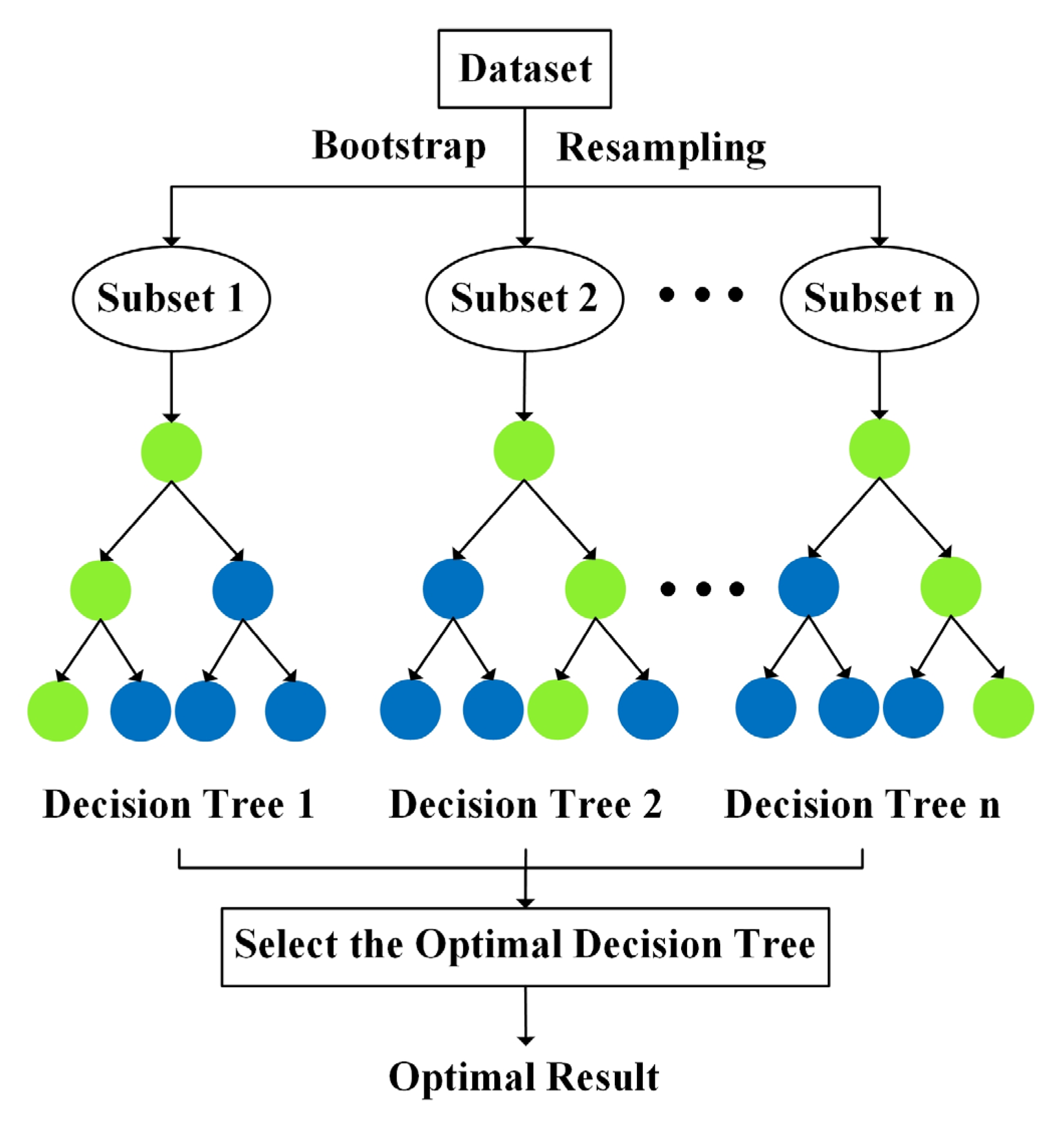
2.3.3. Optimized Random Forest Regression

The random forest regression (RFR) model consists of a multitude of decision trees with no correlation [59], each of which is built as a random sampling process [60]. The use of the bootstrap method in this study, which may cause duplicates in the sample set, is effective in avoiding overfitting and has high accuracy and generalization capacity [61]. Ntree is the number of regression trees. The size of the Ntree value will affect the efficiency and accuracy of the model. Too large, and it will affect the model calculation speed; too small, will cause the error in the model not to stabilize. Mtry is the number of variables used in the node for binary trees, and the choice of the Mtry value directly affects the error rate of the model. Combined with the influence of Ntree and Mtry on the RFR modeling results (Figure 4), the GS method is used to optimize the two hyperparameters, reduce the OBB error value, and construct an ORFR model.

2.3.4. Statistical Analyses

The soil was divided into silty soil and sandy soil according to particle diameter. The correlation between the underground CW-SOC content of the two soil textures and the spectral data were analyzed by the Pearson correlation coefficient [62]. According to the degree of correlation between CW-SOC content and spectral data, the characteristic spectral wavelengths corresponding to silty soil and sandy soil were quickly and accurately selected. It is convenient to further construct a prediction model of SOC content in coastal wetlands. Correlation analysis has a strong purpose, high precision, and good reliability. A correlation coefficient above 0.7 indicates a very tight relationship. The range from 0.4 to 0.7 indicates that the relationship is close. The range from 0.2 to 0.4 indicates that the relationship is normal.

$$r=\frac{{\sum }_{i=1}^n\left(x_i-\overline{x}\right)\left(y_i-\overline{y}\right)}{\sqrt{{\sum }_{i=1}^n{\left(x_i-x\right)}^2}\sqrt{{{\sum }_{i=1}^n\left(y_i-y\right)}^2}}$$

(4)

where x_i indicates the spectral reflectance value, $\overline{x}$ indicates the average measured value of spectral reflectance value, y_i indicates the measured value of soil organic carbon, $\overline{y}$ indicates the average measured value of soil organic carbon, and n indicates the number of samples, i = 1, 2, 3…, n, r indicates the degree of correlation.

2.3.5. Model Validation

The LOO-CV method was used to verify the prediction model of soil organic carbon. The method is a type of K-folding Cross-Validation, which makes K equal to the amount of data in the data set. Only one test set is used each time, and the rest are used as training sets [63]. The results obtained by this method are closest to the expected value of training the whole test set, which is suitable for the small sample data based on this study (Figure 5).

The test accuracy of the model was evaluated by the adjusted coefficient of determination (Adjusted-R²), root mean square error (RMSE), and residual predictive deviation (RPD) of the predicted value and the measured value [64]. The larger the Adjusted-R² is, the smaller the RMSE is, indicating a higher model estimation accuracy. RPD values can be used to explain the predictive power of the model. When RPD < 1.4 it indicates that the model cannot accurately predict; when 1.4 ≤ RPD < 2.0, it indicates that the prediction ability of the model is average; when RPD ≥ 2.0 [65], it indicates that the model has a good predictive ability. The formula is as follows:

$$R^2=\frac{{\sum }_{i=1}^n{\left({\hat{y}}_i-\overline{y}\right)}^2}{{{\sum }_{i=1}^n\left(y_i-\overline{y}\right)}^2}$$

(5)

$$\mathit{Adjusted}-R^2=1-\frac{\left(1-R^2\right)\left(n-1\right)}{\left(n-k-1\right)}$$

(6)

$$RMSE=\sqrt{\frac{{{\sum }_{i=1}^n\left({\hat{y}}_i-y_i\right)}^2}{n}}$$

(7)

$$RPD=\frac{SD}{RMSE}$$

(8)

where y_i indicates the measured value of soil organic carbon, ${\hat{y}}_i$ indicates the predicted value of soil organic carbon, $\overline{y}$ indicates the average measured value of soil organic carbon, and n indicates the number of samples, i = 1, 2, 3…, n, k is the number of arguments, SD indicates the standard deviation of measured value.

3. Results

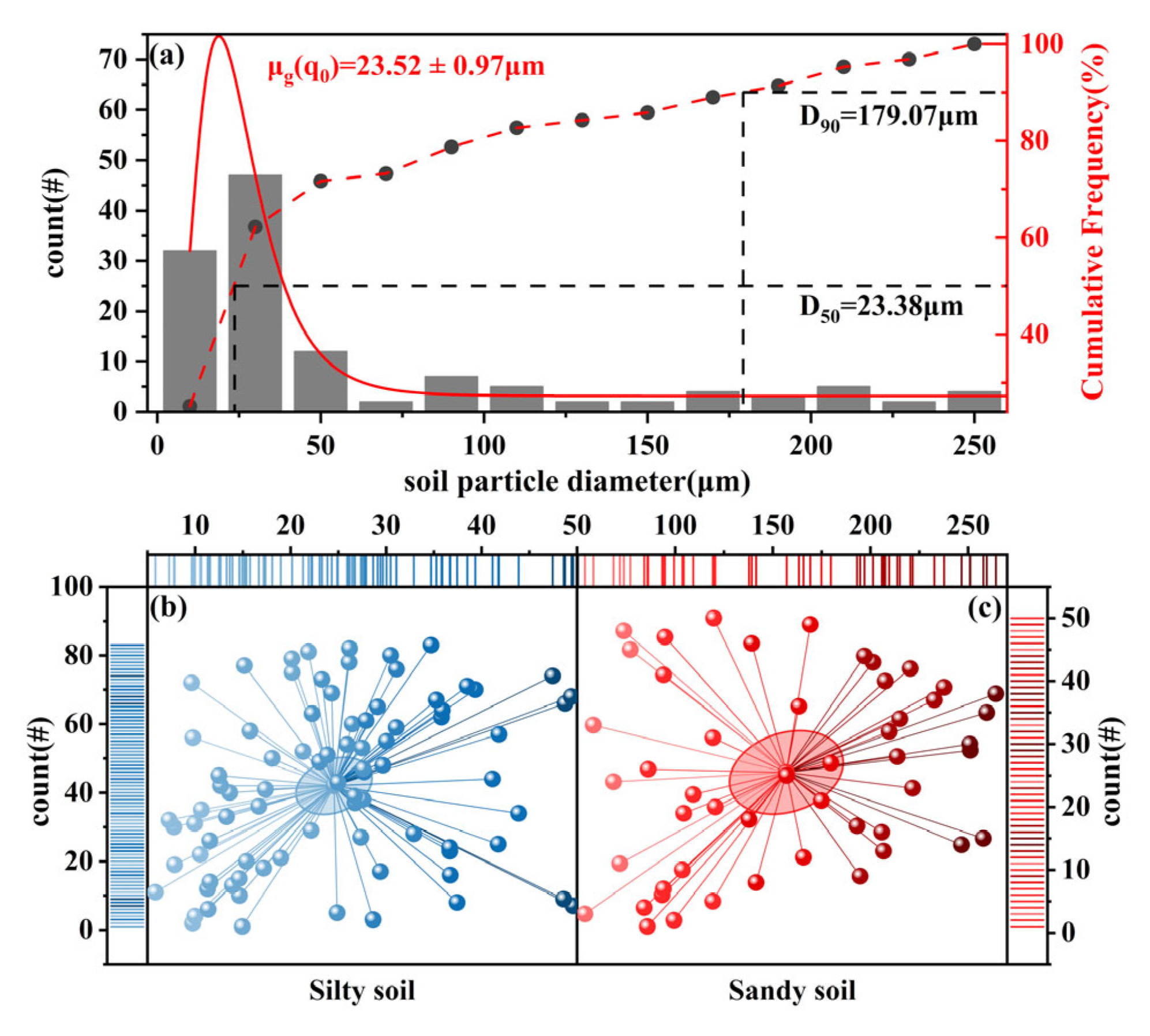
3.1. Descriptive Statistics of CW-SOC

The particle diameter range of topsoil (0~30 cm) of coastal wetlands in the study area is roughly 0~270 μm, while the geometric mean is 23.52 ± 0.97 μm (Figure 6a). This indicates that more than half of the soil particle diameter is below 50 μm. Ninety percent of the soil analyzed had a particle diameter of less than 179.07 μm. According to the classification criteria of soil particle diameter, the collected soils in coastal wetlands are roughly divided into 83 silty soils (Figure 6b) and 50 sandy soils (Figure 6c).

The range of organic carbon content of silty soil presents a standard normal distribution. The organic carbon content of silty soil and sandy soil was significantly different, which met p < 0.01 (

Table 2. CW-SOC’s F-test two-sample for variances.

Soil Texture	Silty	Sandy	Silty and Sandy
mean	8.15	4.51	6.78
variance	12.26	33.32	23.11
observations	83	50	133
df	82	49	131
F	0.67 0.31 × 10−5 0.66
p (F ≤ f) one-tail
F critical one-tail

). The average organic carbon content of silty soils is higher than that of sandy soils, which is about 1.8 times that of sandy soils. The standard deviation (SD) of silty soil and sandy soil were 3.50 and 5.77, respectively. In general, the distribution characteristics of organic carbon content in different types of soil are more obvious. After dividing the samples according to particle diameter, it will be more accurate to establish CW-SOC prediction models for silty soil and sandy soil.

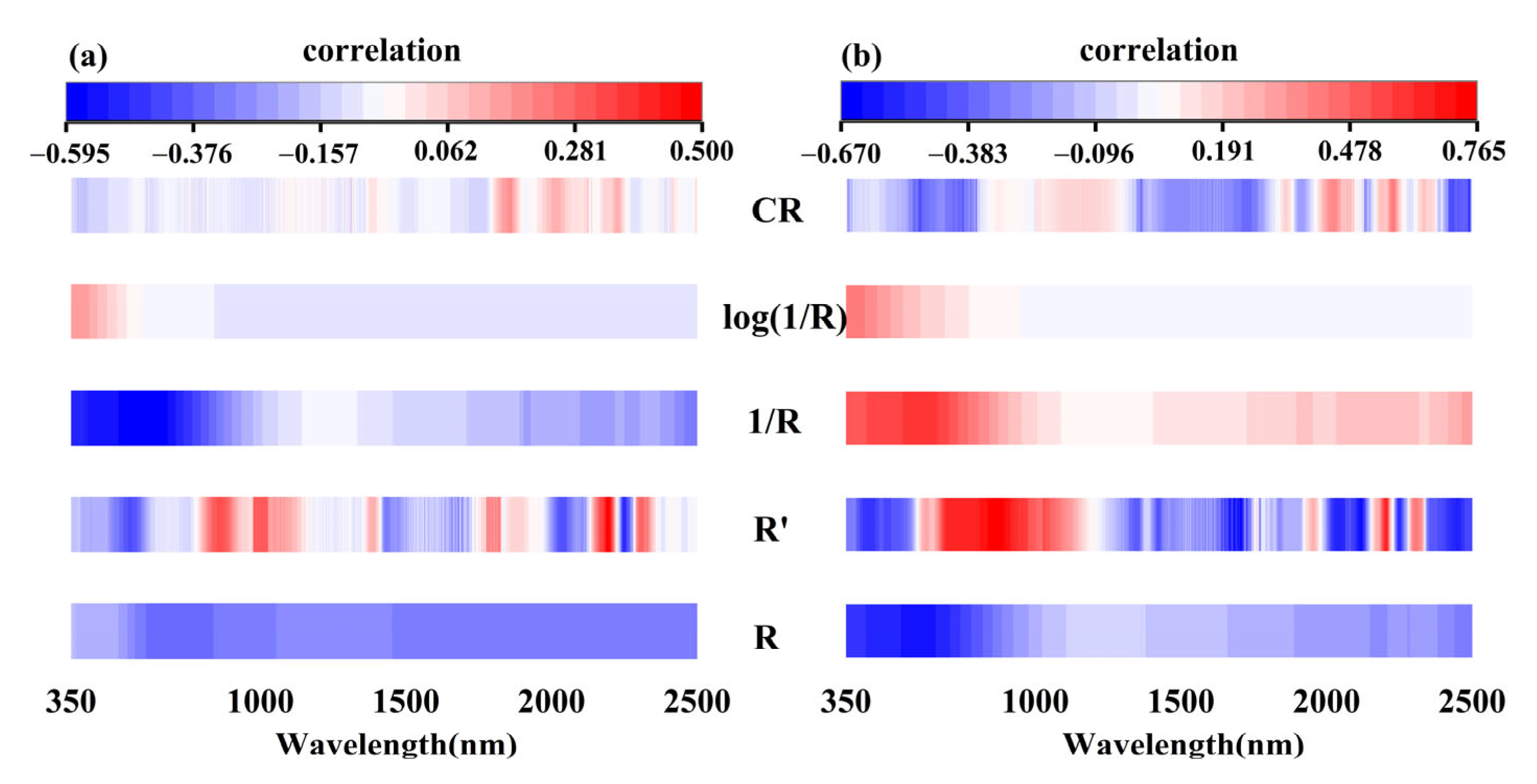
3.2. Selection of CW-SOC Characteristic Wavelengths

The correlation of soil spectral reflectance R, 1/R, log(1/R), R′, CR, and CW-SOC is discussed using two soil textures of coastal wetlands (Figure 7). The 500~1000 nm and 1900~2400 nm spectral intervals are closely related to the CW-SOC selected for silty soil to construct the prediction model of CW-SOC. The 600~1400 nm and 1700~2400 nm spectral intervals were selected for sandy soil. The correlation between CW-SOC and spectrum in sandy soil (Figure 7b) is significantly higher than that in silty soil (Figure 7a). In observing the correlation between CW-SOC content and the corresponding soil spectral reflectance, it was found that there were differences in the degree of correlation between different spectral reflectance transformation methods; log(1/R) had the lowest correlation with CW-SOC, and R′ and 1/R had high correlation with CW-SOC.

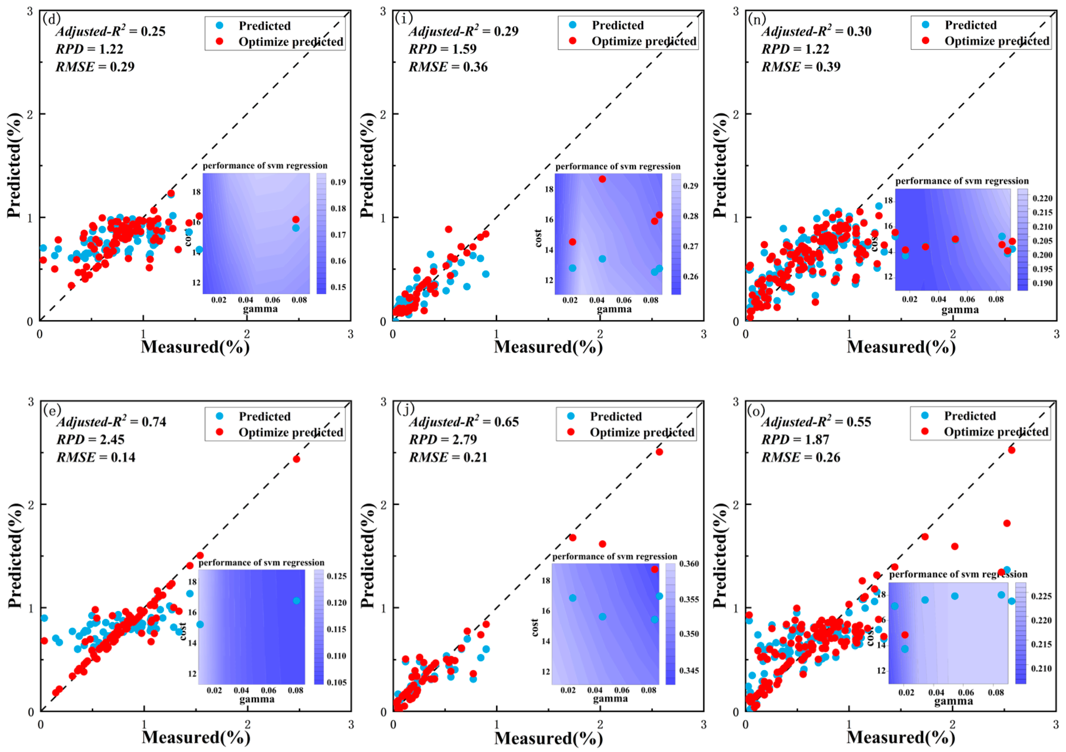
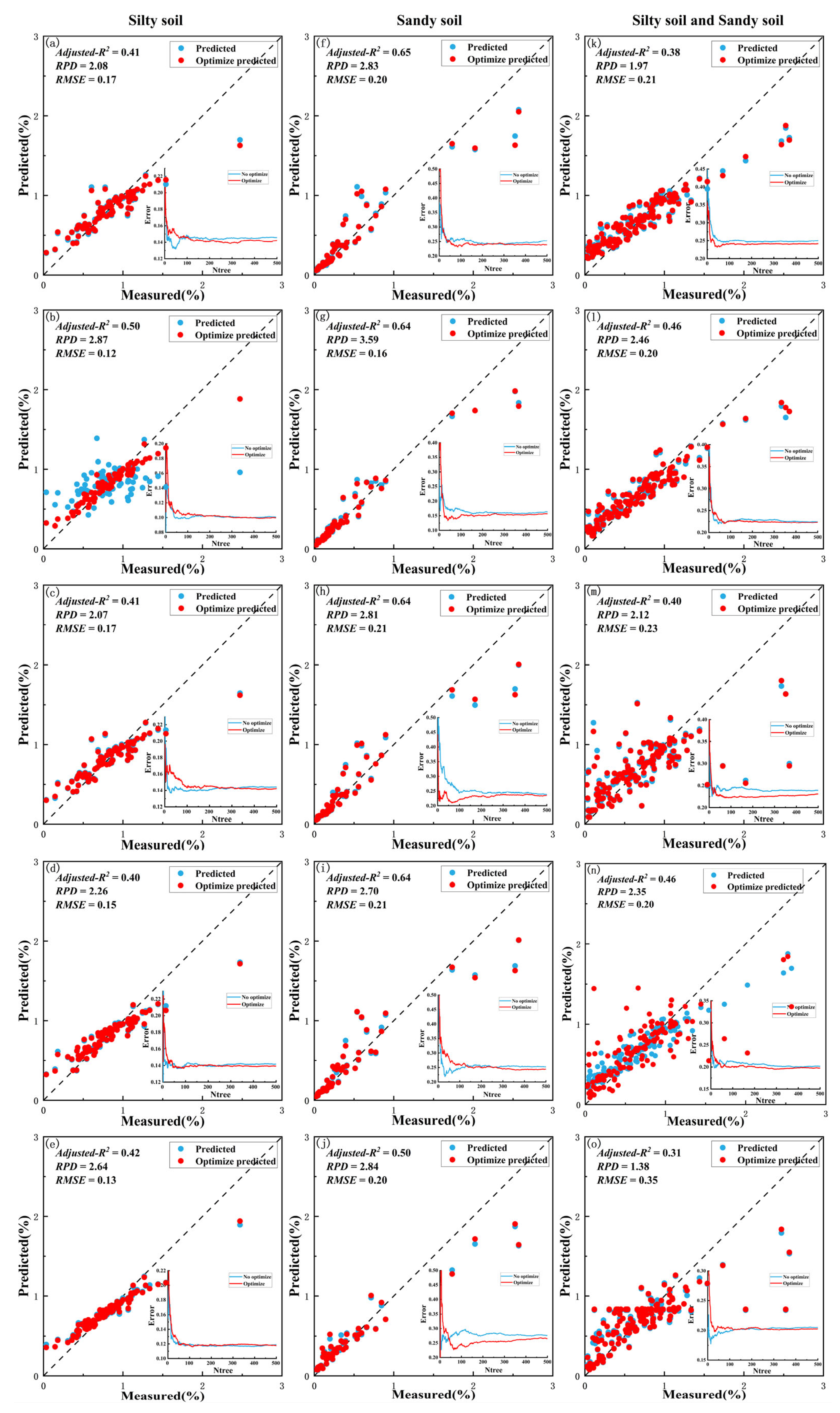
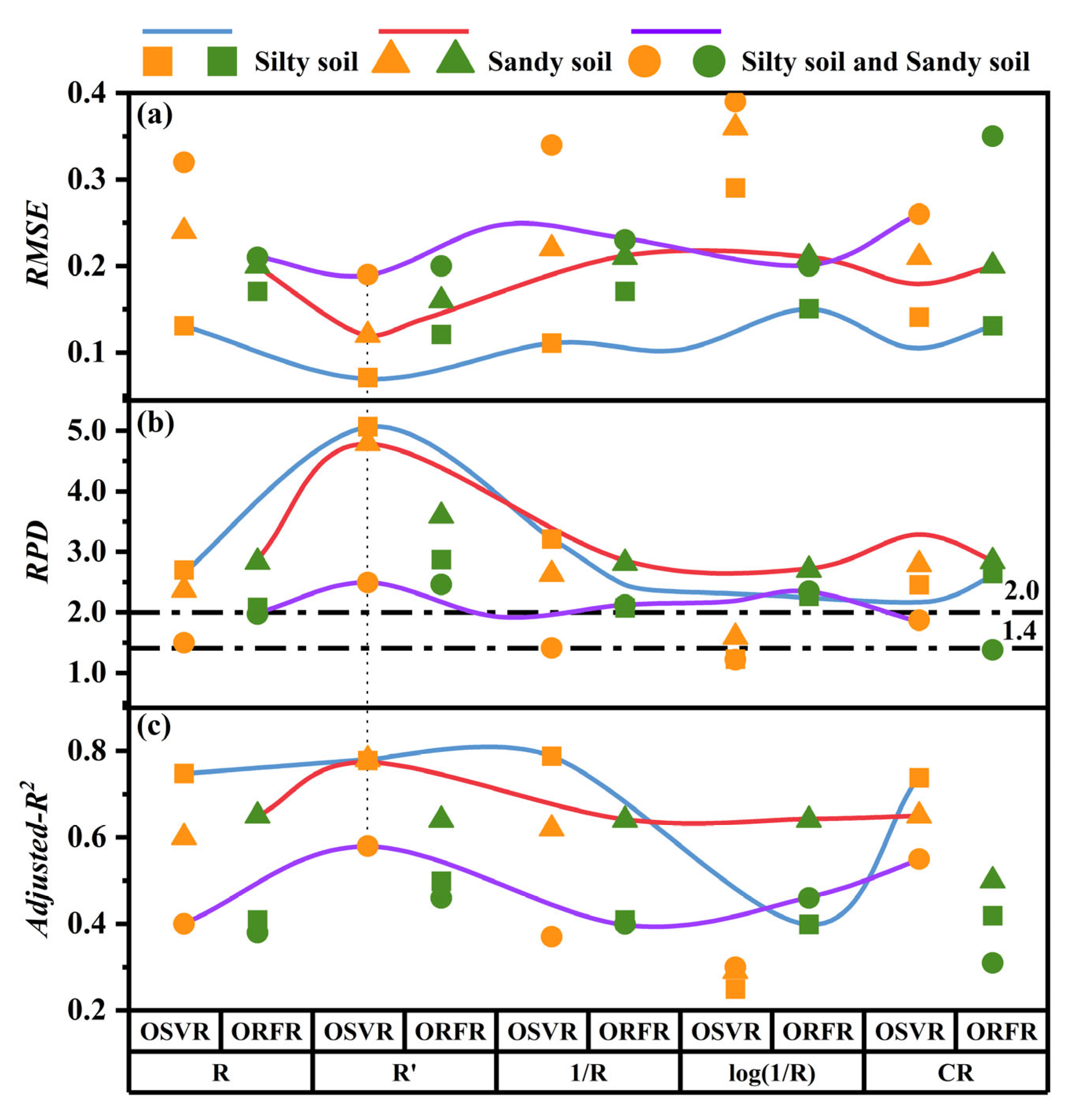
3.3. Model Performance Comparison

Parameters of SVR and RFR models were then optimized (

Table 3. Model optimized parameter.

Texture	Transform Form	OSVR		ORFR
		Cost	Gamma	Ntree	Mtry
silty	R	11	0.09	500	301
	R′	11	0.01	500	451
	1/R	11	0.09	500	301
	log(1/R)	11	0.01	500	301
	CR	19	0.09	500	451
sandy	R	11	0.01	500	651
	R′	11	0.01	500	651
	1/R	11	0.01	500	434
	log(1/R)	17	0.01	500	290
	CR	19	0.09	500	651

). Four CW-SOC models, including SVR, OSVR, RFR, and ORFR, were constructed. The comparison shows that the optimized model results are significantly better than those prior to optimization, so the OSVR model and ORFR model are primarily compared (Figure 8 and Figure 9).

The prediction performance of the OSVR model and ORFR model is based on the leave-one-out method for the two soil textures, including the Adjusted-R², RMSE, and RPD values. When using the OSVR method and ORFR method to establish a CW-SOC model based on VIS-NIR data, it was found that the classification of coastal wetland soil according to soil texture can improve model accuracy, reduce model variability, and improve model performance (Figure 8 and Figure 9). The results showed that both OSVR and ORFR models could significantly improve the performance of the models under two soil textures. For silty sand, the performance of the OSVR model is about 30% higher than that of the traditional SVR model, and the performance of the ORFR model is 3% higher than that of the RFR model. For sandy soil, the performance of the OSVR model is about 15% higher than that of the traditional SVR model, and the performance of the ORFR model is 5% higher than that of the RFR model. Regardless of whether it is silty or sandy soil, the CW-SOC model established under both methods improved the performance of the corresponding model after optimization than before optimization.

The OSVR model based on CW-SOC obtained better results (Figure 8 and Figure 9). Except for the modeling results under the log(1/R) spectral reflectance, the Adjusted-R² values were all over 0.6, and the RMSE value was about 40% lower than the original data (Figure 8). It has also been verified that the essence of the OSVR model to optimize the SVR model by adjusting the parameters Cost and Gamma is to continuously reduce the model error.

Figure 9 shows the optimized results of the ORFR model under two soil textures. The comparison between ORFR and OSVR shows that the optimized degree of the ORFR model is not as significant as that of the OSVR model. Still, the ORFR model also achieves the purpose of optimizing the model. The ORFR model also adjusts parameters Ntree and Ntry to reduce OBB error to improve the model performance. The Adjusted-R² values are all greater than 0.4, and the highest value is 0.65, and the RPD values are all above 2.0, indicating that the model is stable and the uncertainty of the model has been reduced.

According to the research and analysis of this paper, a detailed comparison of OSVR and ORFR methods shows that the CW-SOC content estimation model established by the OSVR method has achieved optimal results, and the results of the OSVR model are better than that of the ORFR model (Figure 10).

The results show that both methods can be used for modeling CW-SOC content and that the organic carbon prediction model of silty soil based on the OSVR method under R′ transformation is the best. The Adjusted-R² value is as high as 0.78, the RPD value is 5.07, model stability is high, RMSE value is as low as 0.07 (Figure 10). The study found that the performance of the OSVR model is significantly higher than that of the SVR model, and the performance of the ORFR model is slightly higher than that of the RFR model, both of which achieved the purpose of improving the performance of the model (Figure 8 and Figure 9).

4. Discussion

4.1. CW-SOC Content of Different Soil Textures

SOC plays a vital role in the carbon cycle, slowing the rate of global warming [66]. There are regional differences in the SOC content in China, and its distribution gradually increases from south to north [67]. Factors such as temperature, precipitation, environmental characteristics, soil nutrients, human activities, and vegetation cover contribute to differences in SOC content [9,10,11]. Additionally, the impact of soil texture on SOC is also very significant due to the unique location of coastal wetlands [67]. When the CW-SOC model was established based on VIS-NIR, 133 soil samples of coastal wetlands were divided into silty soil and sandy soil according to soil texture, and the CW-SOC content was predicted. The CW-SOC model established by the silty mixed soil is significantly less accurate than the prediction of SOC content based on soil texture classification. This is consistent with the findings of a study in which mangrove SOC reserves were underestimated by about 37% in mixed silt soil [68]. A new framework for exploring SOC content based on soil textures in different coastal wetlands has gradually been proposed, revealing that soil texture is a key factor influencing SOC [69,70]. The SOC content is generally considered to be proportional to clay and powder but inversely proportional to the sand content [71,72]. The organic carbon content of soil of different textures varies [73]. This study also found that the organic carbon content of silty soil and sandy soil in coastal wetland soil is significantly different, and the organic carbon content of silty soil is about 1.8 times that of sandy soil. Therefore, soil texture should be explicitly considered when predicting CW-SOC content, analyzing potential future carbon cycles, and sequestration.

4.2. Spectral Feature Wavelengths of CW-SOC

When modeling and predicting CW-SOC content based on VIS-NIR spectral data, it was found that the characteristic wavelengths associated with organic carbon in silty soil were mainly in the spectral range of 500–1000 nm and 1900–2400 nm, and the spectral range of sandy soil was mainly in the spectral range of 600–1400 nm and 1700–2400 nm. Comprehensive exploration shows that the characteristic wavelengths of CW-SOC are roughly consistent with previous findings [4,74,75] and intersect with the SOC spectral characteristic wavelengths of coastal solonchaks.

In this paper, we found that there are differences in the wavelengths of SOC spectroscopic characteristics of different soil types (

Table 4. SOC characteristic wavelengths for different types of soils.

Soil Type	Characteristic Wavelength (nm)	References
field-moist soil	400–800, 1380–1440, 1830–1950, 2090–2400	[78]
cropland soil	450–619, 760–909, 1968–2001	[79]
spartina alterniflora wetland soil	1400, 1900, 2200	[4]
desert wetland soil	745–910, 1911–2254	[74]
coastal solonchaks	1420, 1920, 2210	[75]

), and it is speculated that soil types can affect SOC spectral data. Previous studies have shown that soil type [75], soil texture [76], soil organic matter composition, and organic matter (e.g., aliphatic C–H, cellulose, and lignin in soil [77]) can have an impact on SOC spectroscopic data, which affect the spectrum between 2340 and 2447 nm. At the same time, this study found that under the coastal wetland soil, there are differences in the wavelengths of organic carbon characteristics of silty soil and sandy soil, which is caused by the difference in soil texture.

4.3. Model Algorithm Comparison Evaluation

Compared with traditional chemical experiments, the method of building models to obtain CW-SOC content has the advantages of high efficiency, environmental protection, low labor intensity, and safety and is considered to be a promising use of technology [80,81,82]. SVM and RF algorithms have been widely used to solve complex regression problems, and the model estimation accuracy under the two methods is significantly improved compared with ordinary linear methods [40,83]. Many studies have reported that RFR achieved better results in predicting SOC content compared with multiple linear regression (MLR); SVR prediction SOC content results are also significantly better than partial least squares regression (PLSR) (

Table 5. Comparison of results of different regression methods.

Regression Method	R2	RMSE	References
MLR	0.79	1.44	[39]
RFR	0.97	0.66
PLSR	0.88	0.46	[81]
SVR	0.92	0.36

). During this study, hyperparameter Cost and Gamma in the SVR method and the hyperparameters Ntree and Mtry in the RFR method were further adjusted. It was found that the OSVR and ORFR methods can avoid the phenomenon of overfitting [84] that may occur in the SVR and RFR methods, improving the performance of predicting CW-SOC models. The results show that the performance of the model established by the OSVR method is about 15–30% higher than that of the SVR model. The performance of the model built by the ORFR method is about 3–5% higher than that of the RFR model. Based on OSVR and ORFR methods, the spectral data of VIS-NIR can be used to better predict CW-SOC content.

Some findings suggest that the SVR method achieves the highest performance in SOC estimation among nine commonly used multivariate methods [85,86]. Similarly, this paper concludes that the CW-SOC prediction model based on the OSVR method is superior to the ORFR method. The reason for this can be attributed to two aspects: the application of the SVR model is flexible, and the OSVR has the ability to adjust hyperparameters. SVR models can account for outliers and help solve complex nonlinear regression problems [87]. OSVR can adjust the hyperparameters using the GS method to improve the prediction accuracy of the CW-SOC content.

In this study, based on field sampling data and VIS-NIR spectral data, two optimized machine algorithms were used—OSVR and ORFR method—to establish a CW-SOC prediction model to obtain SOC content efficiently and conveniently. Based on the principles and advantages of OSVR and ORFR models, these models can provide an effective method to retrieve the spatial distribution map of SOC using satellite remote sensing data in a further study [88], for instance, SOC retrieval for simulated Sentinel-2 data using VIS-NIR spectral data based on OSVR and PRFR methods. In addition, OSVR and ORFR models can serve as remote sensing images to retrieve SOC spatial distribution maps [89,90].

5. Conclusions

Taking the coastal areas of Tangshan and Qinhuangdao as the research area, based on the field sampling data and laboratory-measured spectra, the prediction model of topsoil organic carbon in coastal wetlands was established by using optimized machine algorithms OSVR and ORFR. Through the comparison of OSVR, ORFR, SVR, and RFR methods, it is found that OSVR and ORFR methods can improve the performance of the model and are effective methods for modeling soil organic carbon in coastal wetlands. The results are as follows:

(1)

The correlation between organic carbon content and the spectrum of sandy soil in coastal wetlands is significantly higher than that of silty soil. The characteristic wavelengths related to SOC of silty soil are mainly in the spectral range of 500~1000 nm and 1900~2400 nm, and that of sandy soil is mainly in the spectral range of 600~1400 nm and 1700~2400 nm.

(2)

In comparing the two methods, the OSVR method has been proven better than the ORFR method. The organic carbon prediction model of silty soil based on the OSVR method under the R′ transformation is the best, with the Adjusted-R² value as high as 0.78, the RPD value is much greater than 2.0 and 5.07, and the RMSE value as low as 0.07. Both OSVR and ORFR methods can improve the prediction results of the model. OSVR method can improve the performance of the model by about 15~30%, and the ORFR method can improve by about 3~5%. OSVR method is better than the ORFR method.

(3)

The OSVR and ORFR can be used as better methods to accurately predict the soil organic carbon content of coastal wetlands and provide data support for the carbon cycle, soil conservation, plant growth, and environmental protection of coastal wetlands.

References

1. Ortega, A.; Geraldi, N.R.; Alam, I.; Kamau, A.A.; Acinas, S.G.; Logares, R.; Gasol, J.M.; Massana, R.; Krause-Jensen, D.; Duarte, C.M. Important contribution of macroalgae to oceanic carbon sequestration. Nat. Geosci. 2019, 12, 748–754. [Google Scholar] [CrossRef]
2. Kottkamp, A.I.; Jones, C.N.; Palmer, M.A.; Tully, K.L. Physical protection in aggregates and organo-mineral associations contribute to carbon stabilization at the transition zone of seasonally saturated wetlands. Wetlands 2022, 42, 40. [Google Scholar] [CrossRef]
3. Xia, S.; Song, Z.; Van Zwieten, L.; Guo, L.; Yu, C.; Wang, W.; Li, Q.; Hartley, I.P.; Yang, Y.; Liu, H.; et al. Storage, patterns and influencing factors for soil organic carbon in coastal wetlands of china. Glob. Chang. Biol. 2022. [Google Scholar] [CrossRef] [PubMed]
4. Chen, Q.; Yang, R.; Zhu, C. Vis-nir spectroscopy-based prediction of soil organic carbon in coastal wetland invaded by spartina alterniflora. Acta Pedol. Sin. 2021, 58, 694–703. [Google Scholar]
5. He, M.; Mo, X.; Meng, W.; Li, H.; Xu, W.; Huang, Z. Optimization of nitrogen, water and salinity for maximizing soil organic carbon in coastal wetlands. Glob. Ecol. Conserv. 2022, 36, e02146. [Google Scholar] [CrossRef]
6. Minick, K.J.; Mitra, B.; Li, X.; Fischer, M.; Aguilos, M.; Prajapati, P.; Noormets, A.; King, J.S. Wetland microtopography alters response of potential net co2 and ch4 production to temperature and moisture: Evidence from a laboratory experiment. Geoderma 2021, 402, 115367. [Google Scholar] [CrossRef]
7. Zhang, Z.; Wang, Y.; Zhu, Y.; He, K.; Li, T.; Mishra, U.; Peng, Y.; Wang, F.; Yu, L.; Zhao, X.; et al. Carbon sequestration in soil and biomass under native and non-native mangrove ecosystems. Plant Soil 2022. [Google Scholar] [CrossRef]
8. Liu, X.; Lu, X.; Yu, R.; Sun, H.; Li, X.; Li, X.; Qi, Z.; Liu, T.; Lu, C. Distribution and storage of soil organic and inorganic carbon in steppe riparian wetlands under human activity pressure. Ecol. Indic. 2022, 139, 108945. [Google Scholar] [CrossRef]
9. Li, J.; Han, G.; Wang, G.; Liu, X.; Zhang, Q.; Chen, Y.; Song, W.; Qu, W.; Chu, X.; Li, P. Imbalanced nitrogen-phosphorus input alters soil organic carbon storage and mineralisation in a salt marsh. Catena 2022, 208, 105720. [Google Scholar] [CrossRef]
10. Wang, G.X.; Ma, H.Y.; Qian, J.; Chang, J. Impact of land use changes on soil carbon, nitrogen and phosphorus and water pollution in an arid region of northwest china. Soil Use Manag. 2004, 20, 32–39. [Google Scholar] [CrossRef]
11. Qi, Q.; Zhang, D.; Zhang, M.; Tong, S.; Wang, W.; An, Y. Spatial distribution of soil organic carbon and total nitrogen in disturbed carex tussock wetland. Ecol. Indic. 2021, 120, 106930. [Google Scholar] [CrossRef]
12. Lei, D.; Jiang, L.; Wu, X.; Liu, W.; Huang, R. Soil organic carbon and its controlling factors in the lakeside of west mauri lake along the wetland vegetation types. Processes 2022, 10, 765. [Google Scholar] [CrossRef]
13. Mao, D.H.; Wang, Z.M.; Li, L.; Miao, Z.H.; Ma, W.H.; Song, C.C.; Ren, C.Y.; Jia, M.M. Soil organic carbon in the sanjiang plain of china: Storage, distribution and controlling factors. Biogeosciences 2015, 12, 1635–1645. [Google Scholar] [CrossRef]
14. Trumbore, S.E.; Czimczik, C.I. An uncertain future for soil carbon. Science 2008, 321, 1455–1456. [Google Scholar] [CrossRef]
15. Liu, X.; Tan, S.; Song, X.; Wu, X.; Zhao, G.; Li, S.; Liang, G. Response of soil organic carbon content to crop rotation and its controls: A global synthesis. Agric. Ecosyst. Environ. 2022, 335, 108017. [Google Scholar] [CrossRef]
16. McKenna, M.D.; Grams, S.E.; Barasha, M.; Antoninka, A.J.; Johnson, N.C. Organic and inorganic soil carbon in a semi-arid rangeland is primarily related to abiotic factors and not livestock grazing. Geoderma 2022, 419, 115844. [Google Scholar] [CrossRef]
17. Paula, R.R.; Calmon, M.; Lopes-Assad, M.L.; Mendonca, E.d.S. Soil organic carbon storage in forest restoration models and environmental conditions. J. For. Res. 2021, 33, 1123–1134. [Google Scholar] [CrossRef]
18. Minasny, B.; McBratney, A.B.; Malone, B.P.; Wheeler, I. Digital mapping of soil carbon. Adv. Agron. 2013, 118, 1–47. [Google Scholar]
19. Ribeiro, S.G.; Teixeira, A.d.S.; de Oliveira, M.R.R.; Costa, M.C.G.; Araujo, I.C.d.S.; Moreira, L.C.J.; Lopes, F.B. Soil organic carbon content prediction using soil-reflected spectra: A comparison of two regression methods. Remote Sens. 2021, 13, 4752. [Google Scholar] [CrossRef]
20. Wang, S.; Zhuang, Q.; Wang, Q.; Jin, X.; Han, C. Mapping stocks of soil organic carbon and soil total nitrogen in Liaoning province of China. Geoderma 2017, 305, 250–263. [Google Scholar] [CrossRef]
21. Stenberg, B.; Rossel, R.A.V.; Mouazen, A.M.; Wetterlind, J. Visible and near infrared spectroscopy in soil science. Adv. Agron. 2010, 107, 163–215. [Google Scholar]
22. Ji, W.J.; Shi, Z.; Huang, J.Y.; Li, S. In situ measurement of some soil properties in paddy soil using visible and near-infrared spectroscopy. PLoS ONE 2014, 9, e105708. [Google Scholar] [CrossRef]
23. Wang, X.F.; Meng, J.H. Research progress and prospect on soil nutrients monitoring with remote sensing. Remote Sens. Technol. Appl. 2016, 30, 1033–1041. [Google Scholar]
24. Meng, X.; Bao, Y.; Liu, J.; Liu, H.; Zhang, X.; Zhang, Y.; Wang, P.; Tang, H.; Kong, F. Regional soil organic carbon prediction model based on a discrete wavelet analysis of hyperspectral satellite data. Int. J. Appl. Earth Obs. Geoinf. 2020, 89, 102111. [Google Scholar] [CrossRef]
25. Ghosh, A.; Das, B.; Reddy, N. Application of vis-nir spectroscopy for estimation of soil organic carbon using different spectral preprocessing techniques and multivariate methods in the middle indo-gangetic plains of india. Geoderma Reg. 2020, 23, e00349. [Google Scholar]
26. Zhang, Z.; Ding, J.; Zhu, C.; Wang, J.; Ma, G.; Ge, X.; Li, Z.; Han, L. Strategies for the efficient estimation of soil organic matter in salt-affected soils through vis-nir spectroscopy: Optimal band combination algorithm and spectral degradation. Geoderma 2021, 382, 114729. [Google Scholar] [CrossRef]
27. Viscarra Rossel, R.A.; Walvoort, D.J.J.; McBratney, A.B.; Janik, L.J.; Skjemstad, J.O. Visible, near infrared, mid infrared or combined diffuse reflectance spectroscopy for simultaneous assessment of various soil properties. Geoderma 2006, 131, 59–75. [Google Scholar] [CrossRef]
28. Cheng, H.; Zhang, H.; Huang, Z.; Xu, Z.; Yang, Q.; Liu, A. Variations of soil organic carbon content along an altitudinal gradient in wuyi mountain. J. For. Environ. 2018, 38, 135–141. [Google Scholar]
29. Peng, Y.; Knadel, M.; Gislum, R.; Schelde, K.; Thomsen, A.; Greve, M.H. Quantification of soc and clay content using visible near-infrared reflectance-mid-infrared reflectance spectroscopy with jack-knifing partial least squares regression. Soil Sci. 2014, 179, 325–332. [Google Scholar] [CrossRef]
30. Dai, F.; Zhou, Q.; Lv, Z.; Wang, X.; Liu, G. Spatial prediction of soil organic matter content integrating artificial neural network and ordinary kriging in tibetan plateau. Ecol. Indic. 2014, 45, 184–194. [Google Scholar] [CrossRef]
31. Guo, P.T.; Li, M.F.; Luo, W.; Tang, Q.F.; Liu, Z.W.; Lin, Z.M. Digital mapping of soil organic matter for rubber plantation at regional scale: An application of random forest plus residuals kriging approach. Geoderma 2015, 237–238, 49–59. [Google Scholar] [CrossRef]
32. Wang, J.; Tiyip, T.; Ding, J.; Zhang, D.; Liu, W.; Wang, F.; Tashpolat, N. Desert soil clay content estimation using reflectance spectroscopy preprocessed by fractional derivative. PLoS ONE 2017, 12, e0184836. [Google Scholar] [CrossRef]
33. Were, K.; Bui, D.T.; Dick, Ø.B.; Singh, B.R. A comparative assessment of support vector regression, artificial neural networks, and random forests for predicting and mapping soil organic carbon stocks across an afromontane landscape. Ecol. Indic. 2015, 52, 394–403. [Google Scholar] [CrossRef]
34. Meng, R.; Dennison, P.E. Spectroscopic analysis of green, desiccated and dead tamarisk canopies. Photogramm. Eng. Remote Sens. 2015, 81, 199–207. [Google Scholar]
35. Nauman, T.W.; Thompson, J.A.; Rasmussen, C. Semi-automated disaggregation of a conventional soil map using knowledge driven data mining and random forests in the sonoran desert, USA. Photogramm. Eng. Remote Sens. 2014, 80, 353–366. [Google Scholar] [CrossRef]
36. Hong, Y.; Chen, Y.; Yu, L.; Liu, Y.; Liu, Y.; Zhang, Y.; Liu, Y.; Cheng, H. Combining fractional order derivative and spectral variable selection for organic matter estimation of homogeneous soil samples by vis–nir spectroscopy. Remote Sens. 2018, 10, 479. [Google Scholar] [CrossRef]
37. Peng, X.; Shi, T.; Song, A.; Chen, Y.; Gao, W. Estimating soil organic carbon using vis/nir spectroscopy with svmr and spa methods. Remote Sens. 2014, 6, 2699–2717. [Google Scholar] [CrossRef] [Green Version]
38. Zeraatpisheh, M.; Ayoubi, S.; Jafari, A.; Tajik, S.; Finke, P. Digital mapping of soil properties using multiple machine learning in a semi-arid region, central iran. Geoderma 2019, 338, 445–452. [Google Scholar] [CrossRef]
39. Zhang, H.; Wu, P.; Yin, A.; Yang, X.; Zhang, M.; Gao, C. Prediction of soil organic carbon in an intensively managed reclamation zone of eastern china: A comparison of multiple linear regressions and the random forest model. Sci. Total Environ. 2017, 592, 704–713. [Google Scholar] [CrossRef]
40. Mountrakis, G.; Im, J.; Ogole, C. Support vector machines in remote sensing: A review. ISPRS J. Photogramm. Remote Sens. 2011, 66, 247–259. [Google Scholar] [CrossRef]
41. Wang, L.; Wang, X.; Wang, D.; Qi, B.; Zheng, S.; Liu, H.; Luo, C.; Li, H.; Meng, L.; Meng, X.; et al. Spatiotemporal changes and driving factors of cultivated soil organic carbon in northern china’s typical agro-pastoral ecotone in the last 30 years. Remote Sens. 2021, 13, 3607. [Google Scholar] [CrossRef]
42. Zhang, Y.; Liu, W.; Wang, X.; Shaheer, M.A. A novel hierarchical hyper-parameter search algorithm based on greedy strategy for wind turbine fault diagnosis. Expert Syst. Appl. 2022, 202, 117473. [Google Scholar] [CrossRef]
43. Kumar, M.; Ang, L.T.; Ho, C.; Soh, S.E.; Tan, K.H.; Chan, J.K.Y.; Godfrey, K.M.; Chan, S.-Y.; Chong, Y.S.; Eriksson, J.G.; et al. Machine learning-derived prenatal predictive risk model to guide intervention and prevent the progression of gestational diabetes mellitus to type 2 diabetes: Prediction model development study. JMIR Diabetes 2022, 7, e32366. [Google Scholar] [CrossRef]
44. Ahmed, A.; Ashour, O.; Ali, H.; Firouz, M. An integrated optimization and machine learning approach to predict the admission status of emergency patients. Expert Syst. Appl. 2022, 202, 117314. [Google Scholar] [CrossRef]
45. Bhattacharjee, A.; Murugan, R.; Soni, B.; Goel, T. Ada-gridrf: A fast and automated adaptive boost based grid search optimized random forest ensemble model for lung cancer detection. Phys. Eng. Sci. Med. 2022. [Google Scholar] [CrossRef]
46. Navidpour, A.H.; Hosseinzadeh, A.; Huang, Z.; Li, D.; Zhou, J.L. Application of machine learning algorithms in predicting the photocatalytic degradation of perfluorooctanoic acid. Catal. Rev. -Sci. Eng. 2022. [Google Scholar] [CrossRef]
47. Todorov, B.; Billah, A.H.M.M. Post-earthquake seismic capacity estimation of reinforced concrete bridge piers using machine learning techniques. Structures 2022, 41, 1190–1206. [Google Scholar] [CrossRef]
48. Wang, X.; Zhou, X.; Li, B.; Zhang, F.; Zhou, X. A bent line tobit regression model with application to household financial assets. J. Stat. Plan. Inference 2022, 221, 69–80. [Google Scholar] [CrossRef]
49. Aboutalebi, M.; Torres-Rua, A.F.; McKee, M.; Kustas, W.P.; Nieto, H.; Alsina, M.M.; White, A.; Prueger, J.H.; McKee, L.; Alfieri, J.; et al. Downscaling uav land surface temperature using a coupled wavelet-machine learning-optimization algorithm and its impact on evapotranspiration. Irrig. Sci. 2022. [Google Scholar] [CrossRef]
50. Lin, L.; Liu, X. Soil-moisture-index spectrum reconstruction improves partial least squares regression of spectral analysis of soil organic carbon. Precis. Agric. 2022, 23, 1707–1719. [Google Scholar] [CrossRef]
51. Datta, A.; Setia, R.; Barman, A.; Guo, Y.; Basak, N. Carbon dynamics in salt-affected soils. In Research Developments in Saline Agriculture; Springer: Berlin/Heidelberg, Germany, 2019; pp. 369–389. [Google Scholar]
52. Liu, K.H.; Zheng, J.K.; PachecoTorgal, F.; Zhao, X.Y. Innovative modeling framework of chloride resistance of recycled aggregate concrete using ensemble-machine-learning methods. Constr. Build. Mater. 2022, 337, 127613. [Google Scholar] [CrossRef]
53. De Luca, G.; Silva, J.M.N.; Di Fazio, S.; Modica, G. Integrated use of sentinel-1 and sentinel-2 data and open-source machine learning algorithms for land cover mapping in a mediterranean region. Eur. J. Remote Sens. 2022, 55, 52–70. [Google Scholar] [CrossRef]
54. Zhao, Z.; Zou, Y.; Liu, P.; Lai, Z.; Wen, L.; Jin, Y. Eis equivalent circuit model prediction using interpretable machine learning and parameter identification using global optimization algorithms. Electrochim. Acta 2022, 418, 140350. [Google Scholar] [CrossRef]
55. Wu, X.; Zuo, W.; Lin, L.; Jia, W.; Zhang, D. F-svm: Combination of feature transformation and svm learning via convex relaxation. IEEE Trans. Neural Netw. Learn. Syst. 2018, 29, 5185–5199. [Google Scholar] [CrossRef] [PubMed]
56. Aghelpour, P.; Mohammadi, B.; Biazar, S.M. Long-term monthly average temperature forecasting in some climate types of iran, using the models sarima, svr, and svr-fa. Theor. Appl. Climatol. 2019, 138, 1471–1480. [Google Scholar] [CrossRef]
57. Thomas, S.; Pillai, G.N.; Pal, K. Prediction of peak ground acceleration using ϵ-svr, ν-svr and ls-svr algorithm. Geomat. Nat. Hazards Risk 2016, 8, 177–193. [Google Scholar] [CrossRef]
58. Li, Y.K.; Tian, Y.J.; Ouyang, Z.Y.; Wang, L.Y.; Xu, T.W.; Yang, P.; Zhao, H.X. Analysis of soil erosion characteristics in small watersheds with particle swarm optimization, support vector machine, and artificial neuronal networks. Environ. Earth Sci. 2010, 60, 1559–1568. [Google Scholar] [CrossRef] [Green Version]
59. Zhang, H.; Wang, M. Search for the smallest random forest. Stat. Interface 2009, 2, 381–388. [Google Scholar]
60. Zhong, Y.; Yang, H.; Zhang, Y.; Li, P. Online rebuilding regression random forests. Knowl. Based Syst. 2021, 221, 106960. [Google Scholar] [CrossRef]
61. Sun, J.; Zhong, G.; Huang, K.; Dong, J. Banzhaf random forests: Cooperative game theory based random forests with consistency. Neural Netw. 2018, 106, 20–29. [Google Scholar] [CrossRef]
62. Edelmann, D.; Móri, T.F.; Székely, G.J. On relationships between the pearson and the distance correlation coefficients. Stat. Probab. Lett. 2021, 169, 108960. [Google Scholar] [CrossRef]
63. Modaresi, F.; Araghinejad, S.; Ebrahimi, K. A comparative assessment of artificial neural network, generalized regression neural network, least-square support vector regression, and k-nearest neighbor regression for monthly streamflow forecasting in linear and nonlinear conditions. Water Resour. Manag. 2018, 32, 243–258. [Google Scholar] [CrossRef]
64. Fernández-Cuesta, Á.; Fernández-Martínez, J.M.; Company, R.S.I.; Velasco, L. Near—infrared spectroscopy for analysis of oil content and fatty acid profile in almond flour. Eur. J. Lipid Sci. Technol. 2012, 115, 211–216. [Google Scholar] [CrossRef]
65. Reda, R.; Saffaj, T.; Derrouz, H.; Itqiq, S.E.; Bouzida, I.; Saidi, O.; Lakssir, B.; El Hadrami, E. Comparing calreg performance with other multivariate methods for estimating selected soil properties from moroccan agricultural regions using nir spectroscopy. Chemom. Intell. Lab. Syst. 2021, 211, 104277. [Google Scholar] [CrossRef]
66. Xiong, J.; Sheng, X.; Wang, M.; Wu, M.; Shao, X. Comparative study of methane emission in the reclamation-restored wetlands and natural marshes in the hangzhou bay coastal wetland. Ecol. Eng. 2022, 175, 106473. [Google Scholar] [CrossRef]
67. Zhang, Y.; Li, P.; Liu, X.; Xiao, L.; Li, T.; Wang, D. The response of soil organic carbon to climate and soil texture in china. Front. Earth Sci. 2022. [Google Scholar] [CrossRef]
68. Wang, Q.; Wen, Y.; Zhao, B.; Hong, H.; Liao, R.; Li, J.; Liu, J.; Lu, H.; Yan, C. Coastal soil texture controls soil organic carbon distribution and storage of mangroves in china. Catena 2021, 207, 105709. [Google Scholar] [CrossRef]
69. Pathak, P.; Reddy, A.S. Vertical distribution analysis of soil organic carbon and total nitrogen in different land use patterns of an agro-organic farm. Trop. Ecol. 2021, 62, 386–397. [Google Scholar] [CrossRef]
70. Riggers, C.; Poeplau, C.; Don, A.; Frühauf, C.; Dechow, R. How much carbon input is required to preserve or increase projected soil organic carbon stocks in german croplands under climate change? Plant Soil 2021, 460, 417–433. [Google Scholar] [CrossRef]
71. Xiao, L.; Liu, G.; Li, P.; Li, Q.; Xue, S. Ecoenzymatic stoichiometry and microbial nutrient limitation during secondary succession of natural grassland on the loess plateau, china. Soil Tillage Res. 2020, 200, 104605. [Google Scholar] [CrossRef]
72. Zhang, Y.; Li, P.; Liu, X.; Xiao, L.; Chang, E.; Su, Y.; Zhang, J.; Liu, Z. Sediment and soil organic carbon loss during continuous extreme scouring events on the loess plateau. Soil Sci. Soc. Am. J. 2020, 84, 1957–1970. [Google Scholar] [CrossRef]
73. Chen, X.H.; Duan, Z.H.; Luo, T.F.; Tan, M.L. The influence of desertification reversal on organic carbon and nutrients distributions in surface soil particle: A case study in yanchi county, ningxia hui autonomous region. Chin. J. Soil Sci. 2014, 45, 1416–1423. [Google Scholar]
74. Ding, J.; Yang, A.; Wang, J.; Sagan, V.; Yu, D. Machine-learning-based quantitative estimation of soil organic carbon content by vis/nir spectroscopy. Peerj 2018, 6. [Google Scholar] [CrossRef]
75. Liu, Y.; Shi, Z.; Zhang, G.; Chen, Y.; Li, S.; Hong, Y.; Shi, T.; Wang, J.; Liu, Y. Application of spectrally derived soil type as ancillary data to improve the estimation of soil organic carbon by using the chinese soil vis-nir spectral library. Remote Sens. 2018, 10, 1747. [Google Scholar] [CrossRef]
76. Moura-Bueno, J.M.; Diniz Dalmolin, R.S.; Horst-Heinen, T.Z.; ten Caten, A.; Vasques, G.M.; Dotto, A.C.; Grunwald, S. When does stratification of a subtropical soil spectral library improve predictions of soil organic carbon content? Sci. Total Environ. 2020, 737, 139895. [Google Scholar] [CrossRef] [PubMed]
77. Knadel, M.; Masis-Melendez, F.; de Jonge, L.W.; Moldrup, P.; Arthur, E.; Greve, M.H. Assessing soil water repellency of a sandy field with visible near infrared spectroscopy. J. Near Infrared Spectrosc. 2016, 24, 215–224. [Google Scholar] [CrossRef]
78. Yu, W.; Hong, Y.; Chen, S.; Chen, Y.; Zhou, L. Comparing two different development methods of external parameter orthogonalization for estimating organic carbon from field-moist intact soils by reflectance spectroscopy. Remote Sens. 2022, 14, 1303. [Google Scholar] [CrossRef]
79. Hu, T.; Qi, K.; Hu, Y. Using vis-nir spectroscopy to estimate soil organic content. In Proceedings of the 38th IEEE International Geoscience and Remote Sensing Symposium (IGARSS), Valencia, Spain, 22–27 July 2018; pp. 8263–8266. [Google Scholar]
80. Ji, W.; Adamchuk, V.I.; Chen, S.; Mat Su, A.S.; Ismail, A.; Gan, Q.; Shi, Z.; Biswas, A. Simultaneous measurement of multiple soil properties through proximal sensor data fusion: A case study. Geoderma 2019, 341, 111–128. [Google Scholar] [CrossRef]
81. Xu, M.; Chu, X.; Fu, Y.; Wang, C.; Wu, S. Improving the accuracy of soil organic carbon content prediction based on visible and near-infrared spectroscopy and machine learning. Environ. Earth Sci. 2021, 80, 326. [Google Scholar] [CrossRef]
82. Zhang, Z.; Ding, J.; Zhu, C.; Wang, J. Combination of efficient signal pre-processing and optimal band combination algorithm to predict soil organic matter through visible and near-infrared spectra. Spectrochim. Acta A Mol. Biomol. Spectrosc. 2020, 240, 118553. [Google Scholar] [CrossRef]
83. Li, H.; Jia, S.; Le, Z. Quantitative analysis of soil total nitrogen using hyperspectral imaging technology with extreme learning machine. Sensors 2019, 19, 4355. [Google Scholar] [CrossRef]
84. Wang, J.; Ding, J.; Abulimiti, A.; Cai, L. Quantitative estimation of soil salinity by means of different modeling methods and visible-near infrared (vis-nir) spectroscopy, ebinur lake wetland, northwest china. PeerJ 2018, 6, e4703. [Google Scholar] [CrossRef]
85. Dotto, A.C.; Dalmolin, R.S.D.; Caten, A.T.; Grunwald, S. A systematic study on the application of scatter-corrective and spectral-derivative preprocessing for multivariate prediction of soil organic carbon by vis-nir spectra. Geoderma 2018, 314, 262–274. [Google Scholar] [CrossRef]
86. Xu, S.; Zhao, Y.; Wang, M.; Shi, X. Comparison of multivariate methods for estimating selected soil properties from intact soil cores of paddy fields by vis–nir spectroscopy. Geoderma 2018, 310, 29–43. [Google Scholar] [CrossRef]
87. Raj, A.; Chakraborty, S.; Duda, B.M.; Weindorf, D.C.; Li, B.; Roy, S.; Sarathjith, M.; Das, B.S.; Paulette, L. Soil mapping via diffuse reflectance spectroscopy based on variable indicators: An ordered predictor selection approach. Geoderma 2018, 314, 146–159. [Google Scholar] [CrossRef]
88. Perich, G.; Aasen, H.; Verrelst, J.; Argento, F.; Walter, A.; Liebisch, F. Crop nitrogen retrieval methods for simulated sentinel-2 data using in-field spectrometer data. Remote Sens. 2021, 13, 2404. [Google Scholar] [CrossRef]
89. Zhou, T.; Geng, Y.; Ji, C.; Xu, X.; Wang, H.; Pan, J.; Bumberger, J.; Haase, D.; Lausch, A. Prediction of soil organic carbon and the c: N ratio on a national scale using machine learning and satellite data: A comparison between sentinel-2, sentinel-3 and landsat-8 images. Sci. Total Environ. 2021, 755, 142661. [Google Scholar] [CrossRef]
90. Pham, T.D.; Yokoya, N.; Nguyen, T.T.T.; Le, N.N.; Ha, N.T.; Xia, J.; Takeuchi, W.; Pham, T.D. Improvement of mangrove soil carbon stocks estimation in north vietnam using sentinel-2 data and machine learning approach. GISci. Remote Sens. 2021, 58, 68–87. [Google Scholar] [CrossRef]
Figure 1. Geographic location of the study area. (a) Sample point distribution; (b) CW-SOC content statistics; (c) Coastal wetland soil.
Remotesensing 14 04372 g001
Figure 2. Soil sample reflectance curve before and after S-G convolution smoothing. (a) Silty Soil: laboratory measured spectra; (b) Sandy Soil: laboratory measured spectra; (c) Silty Soil: S-G convolution smoothing; (d) Sandy Soil: S-G convolution smoothing.
Remotesensing 14 04372 g002
Figure 3. The framework of this study.
Remotesensing 14 04372 g003
Figure 4. ORFR Model Structural Framework.
Remotesensing 14 04372 g004
Figure 5. Schematic diagram of LOO-CV principle.
Remotesensing 14 04372 g005
Figure 6. Statistical map of soil particle diameter in coastal wetlands. (a) Statistical results of soil particle diameter: Dn represents the particle diameter corresponding to n% of the soil; μg(q0) represents the geometric average of soil particle diameter; (b) Particle diameter distribution in silty soils; (c) Particle diameter distribution in sandy soils.
Remotesensing 14 04372 g006
Figure 7. Spectral correlation between SOC and soil. (a) silty soil; (b) sandy soil.
Remotesensing 14 04372 g007
Figure 8. OSVR model results. (ae) are silty soil; (fj) are sandy soil; (ko) are silty soil and sandy soil; the order was R, R′, 1/R, log(1/R), and CR.
Remotesensing 14 04372 g008aRemotesensing 14 04372 g008b
Figure 9. ORFR model results. (ae) are silty soil; (fj) are sandy soil; (ko) are silty soil and sandy soil; the order was R, R′, 1/R, log(1/R), and CR.
Remotesensing 14 04372 g009
Figure 10. Model evaluation comparison. (a) RMSE; (b) RPD; (c) Adjusted-R2.
Remotesensing 14 04372 g010