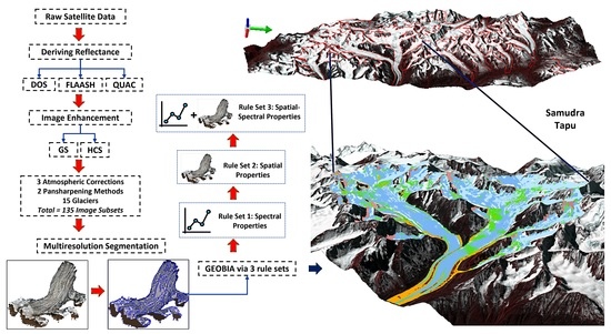
Effect of Image-Processing Routines on Geographic Object-Based Image Analysis for Mapping Glacier Surface Facies from Svalbard and the Himalayas
Abstract
:1. Introduction
GEOBIA
2. Study Areas and Data Used
2.1. Study Sites
2.2. Satellite and Elevation Data
3. Research Methodology
3.1. Experimental Setup
3.2. Processing Routines
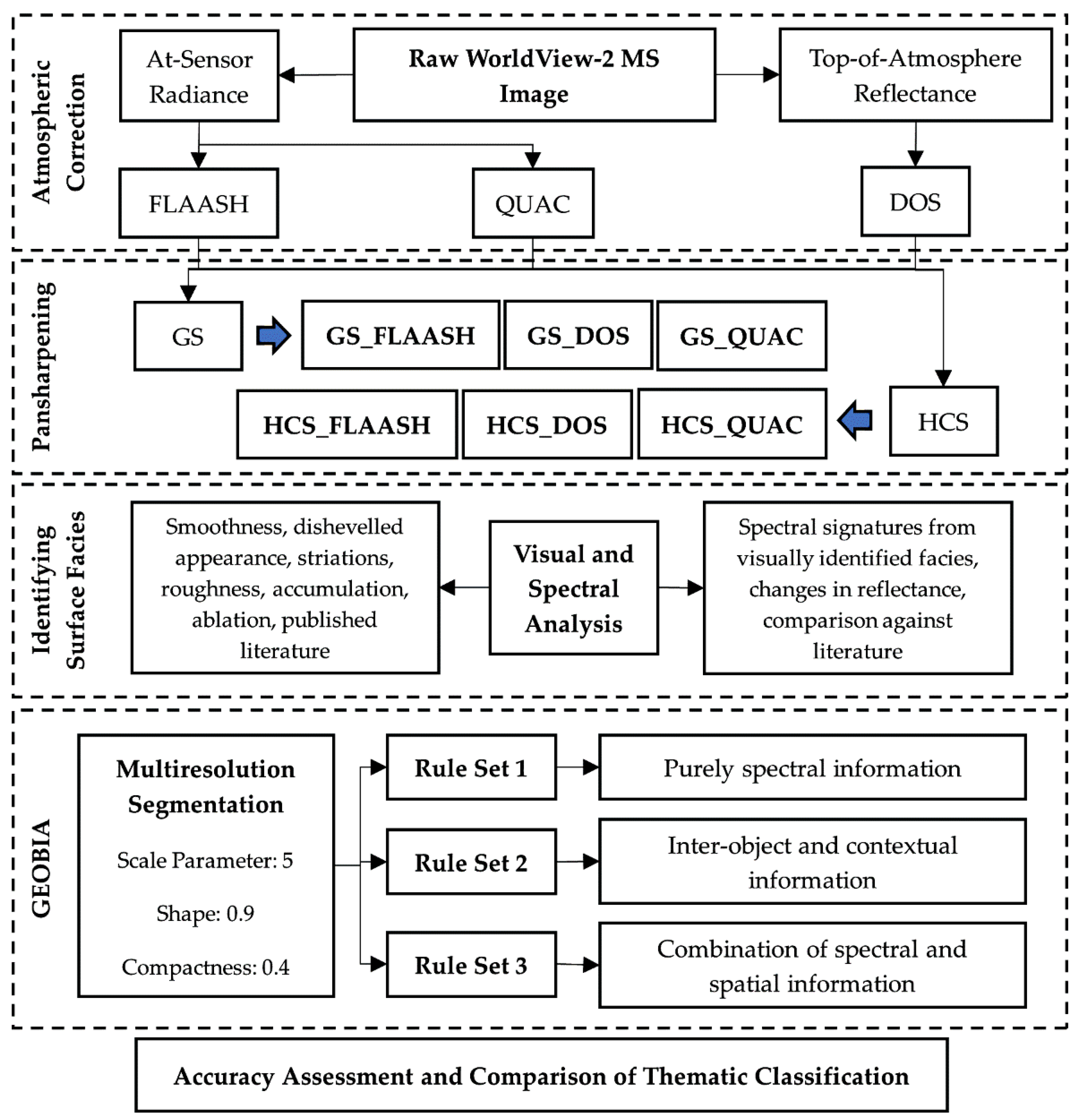
3.2.1. Deriving Reflectance: Radiometric and Atmospheric Corrections
3.2.2. Pansharpening and Glacier Extent Delineation
3.3. Mapping Facies in a GEOBIA Domain
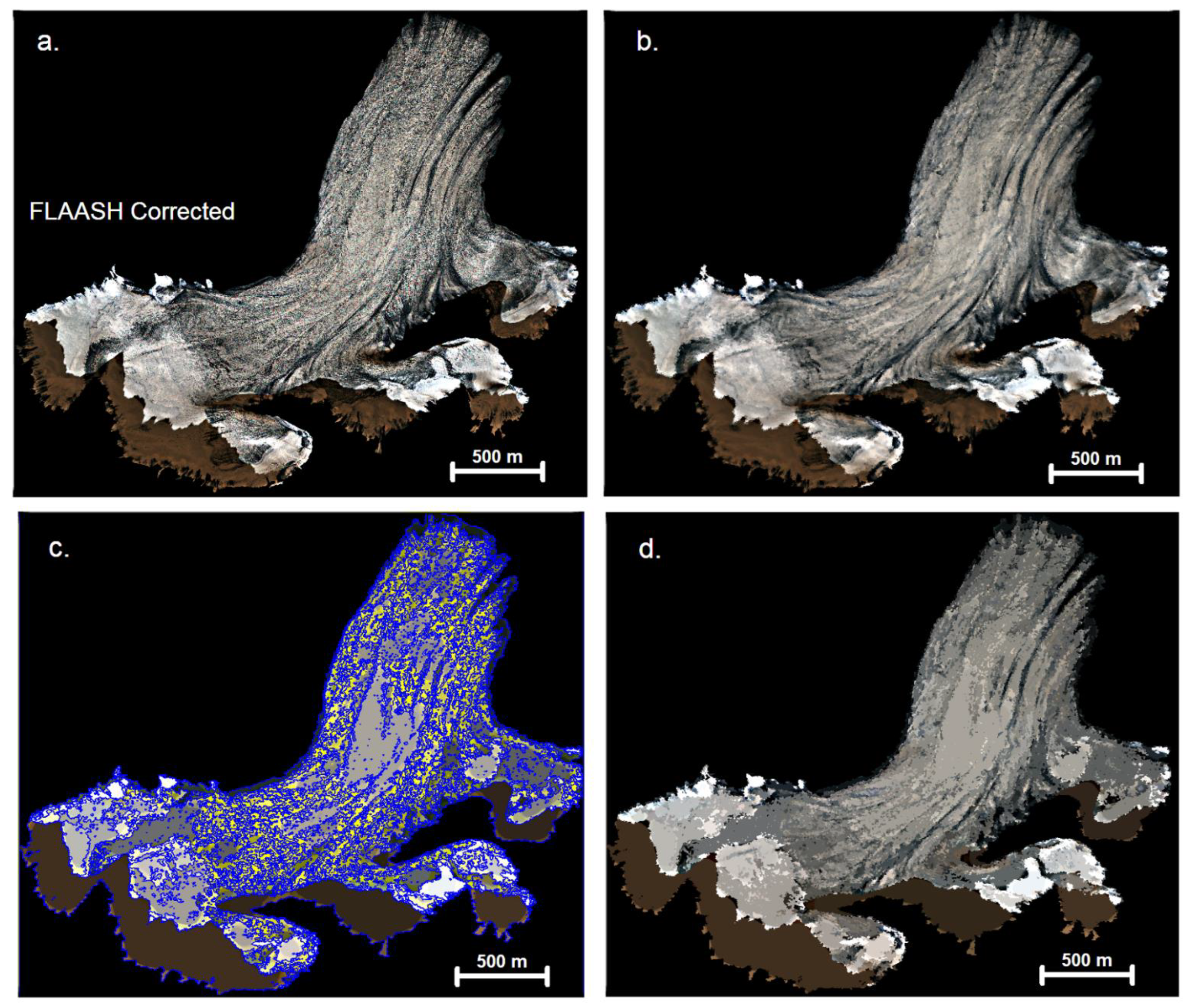
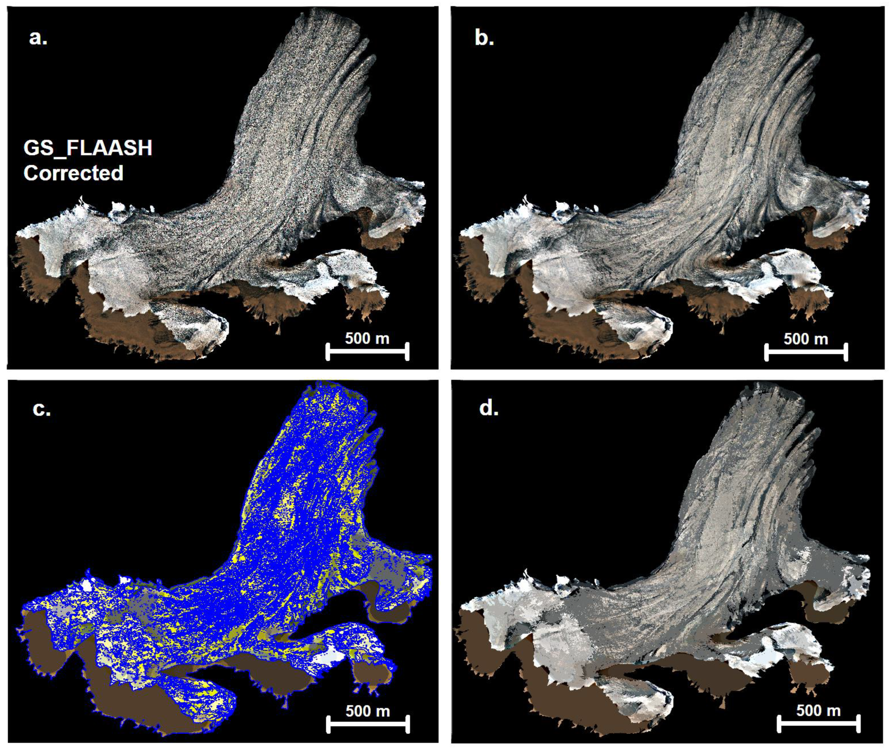
3.3.1. Multiresolution Segmentation
3.3.2. Object Features and Rule Sets
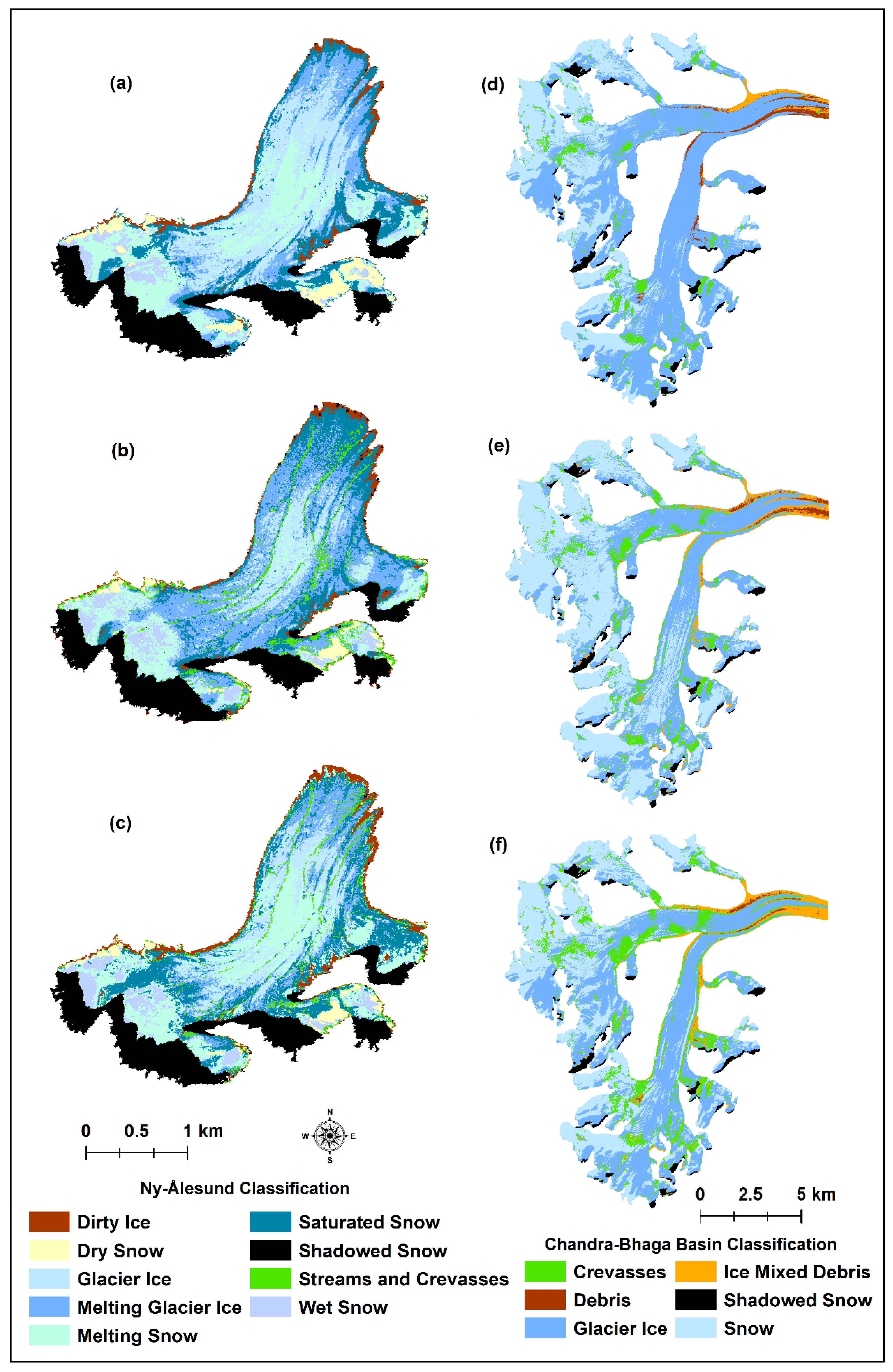
- Rule Set 1: Only object spectral informationThis rule set utilizes only spectral information from the mean values per band and customized ratios developed from the mean values to classify objects, the reasoning being to test the level of accuracy achievable when classifying objects using only spectral properties.
- Rule Set 2: Inter-object and contextual informationThis rule set utilizes features that are not direct object spectral properties or ratioed spectral properties. This rule set will test classification of segmented objects without direct information on the spectral properties of the object.
- Rule Set 3: Combination of spectral and contextual informationThis rule set will attempt to combine the features of both rule sets to achieve the best possible classification map. Supplementary Table S3 presents the exact rule set post segmentation for all the processing schemes. Table 3 highlights the best performing rule sets for the associated processing scheme for both study areas based on individual overall accuracy and F1 score.
3.4. Accuracy Assessment
4. Results and Discussion
4.1. Quantitative Analysis of Surface Facies
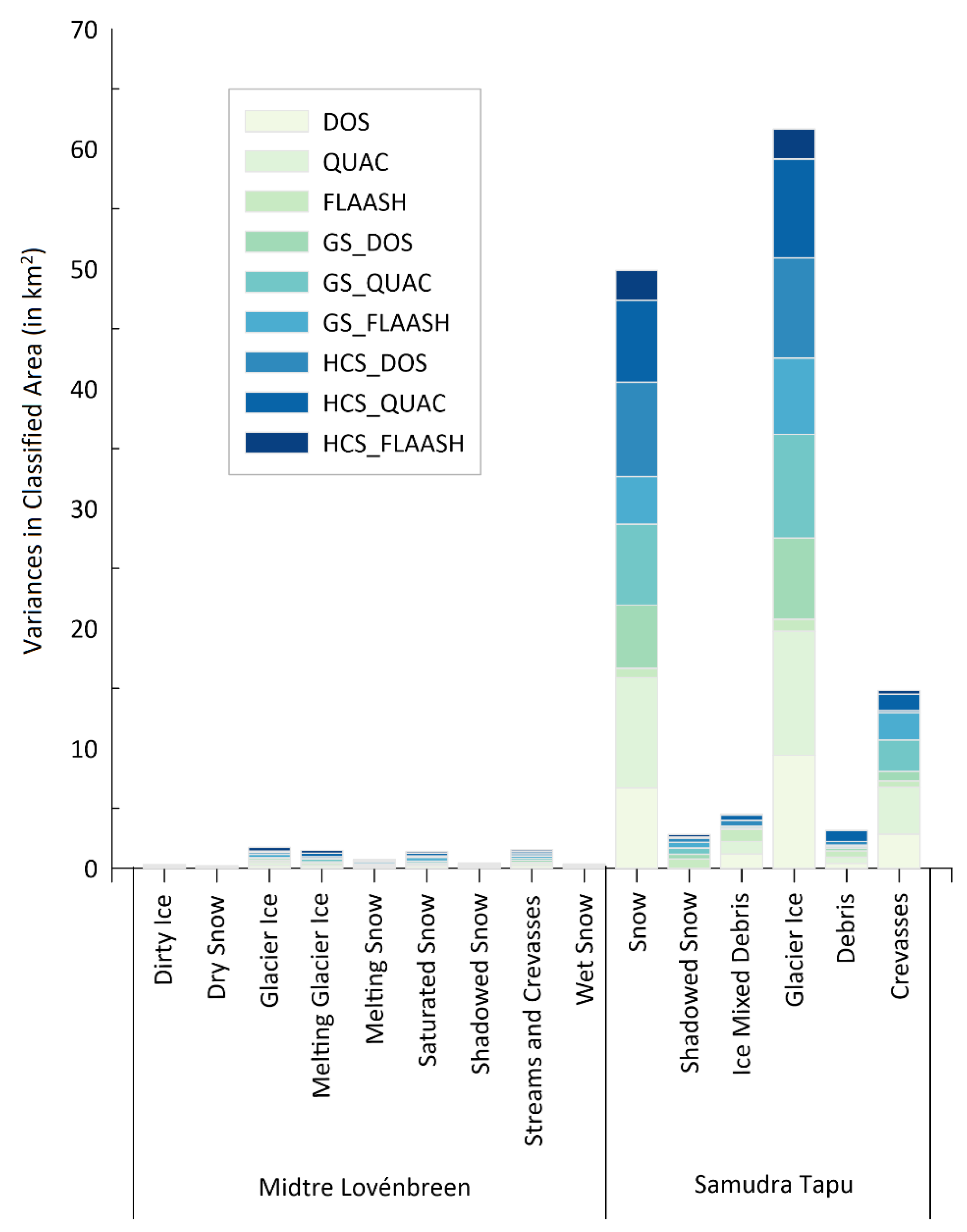
4.1.1. Area of Surface Facies for Each Processing Scheme
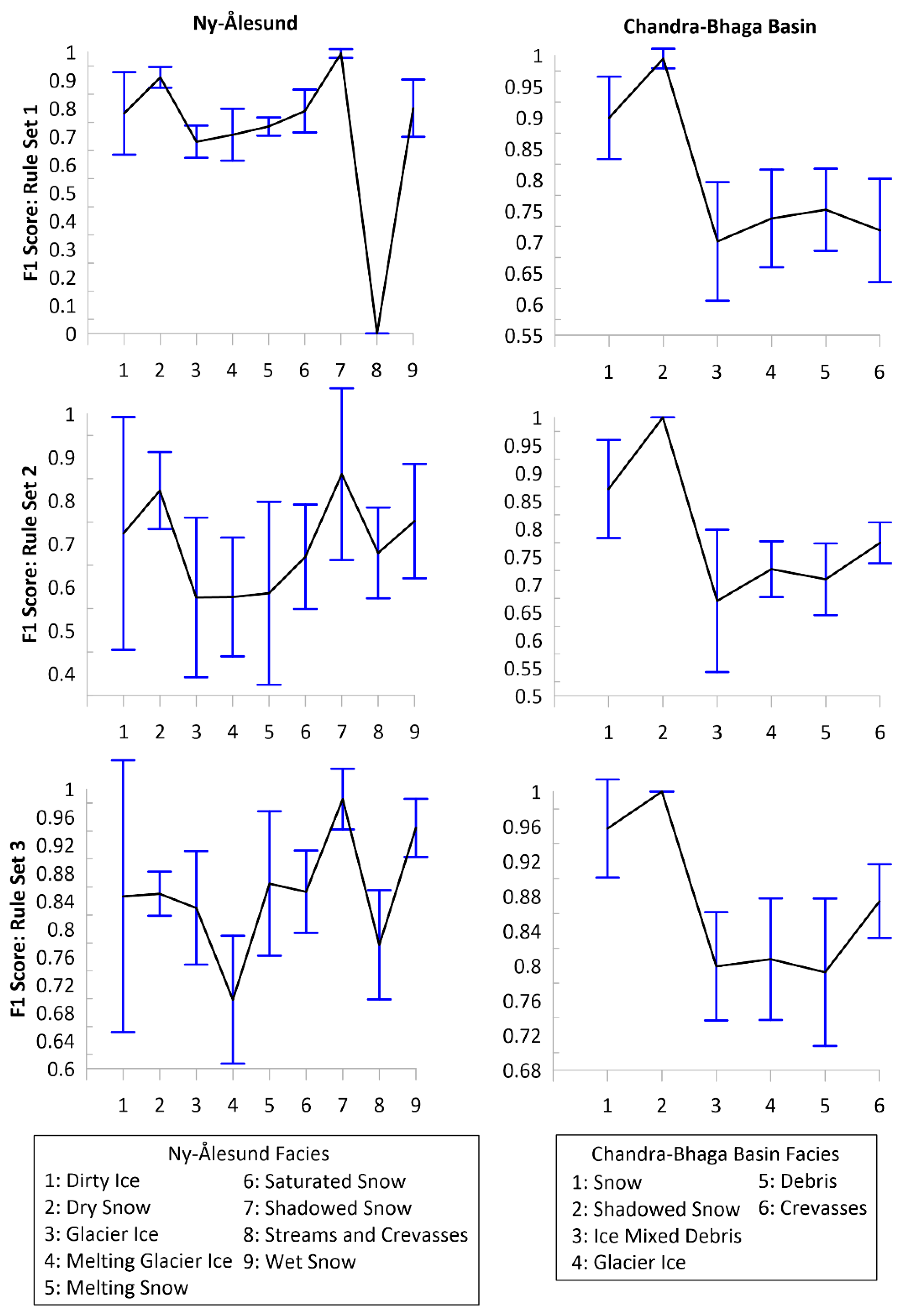
4.1.2. Accuracy Yielded by Each Rule Set
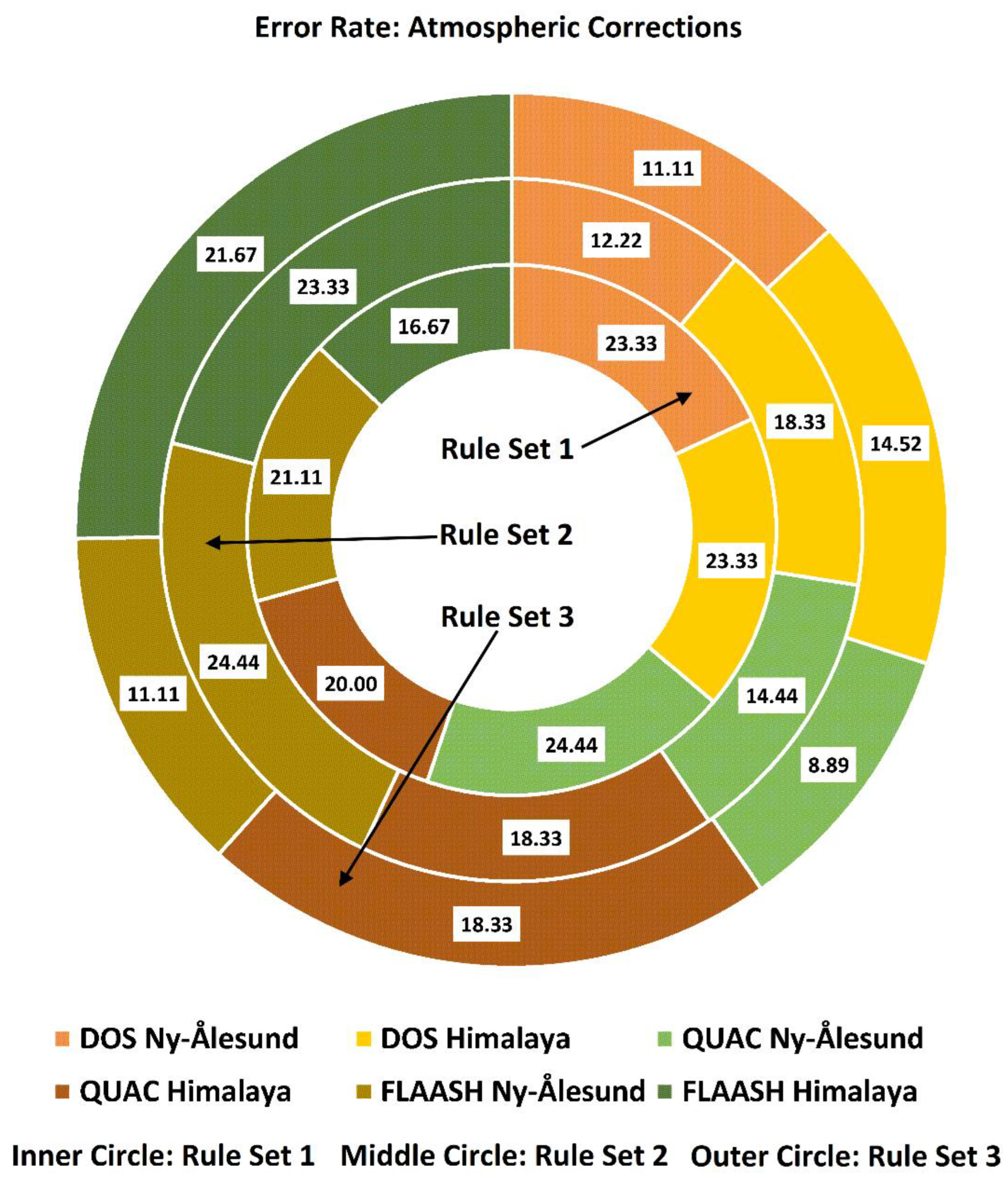
4.1.3. Variable Effect of Atmospheric Corrections
4.1.4. Impact of Pansharpening
4.2. Discussion
Significances and Challenges
5. Conclusions
Supplementary Materials
Author Contributions
Funding
Data Availability Statement
Acknowledgments
Conflicts of Interest
References
- Huss, M. Present and future contribution of glacier storage change to runoff from macroscale drainage basins in Europe. Water Resour. Res. 2011, 47, W07511. [Google Scholar] [CrossRef]
- Kulkarni, A.V.; Randhawa, S.S.; Rathore, B.P.; Bahuguna, I.M.; Sood, R.K. Snow and glacier melt runoff model to estimate hydropower potential. J. Indian Soc. Remote Sens. 2002, 30, 221–228. [Google Scholar] [CrossRef]
- Gaddam, V.K.; Boddapati, R.; Kumar, T.; Kulkarni, A.V.; Bjornsson, H. Application of “OTSU”—An image segmentation method for differentiation of snow and ice regions of glaciers and assessment of mass budget in Chandra basin, Western Himalaya using Remote Sensing and GIS techniques. Environ. Monit. Assess. 2022, 194, 337. [Google Scholar] [CrossRef] [PubMed]
- Bolch, T.; Menounos, B.; Wheate, R. Landsat-based inventory of glaciers in western Canada, 1985–2005. Remote Sens. Environ. 2010, 114, 127–137. [Google Scholar] [CrossRef]
- Gore, A.; Mani, S.; HariRam, R.P.; Shekhar, C.; Ganju, A. Glacier surface characteristics derivation and monitoring using Hyperspectral datasets: A case study of Gepang Gath glacier, Western Himalaya. Geocarto Int. 2017, 34, 23–42. [Google Scholar] [CrossRef]
- Braun, M.; Schuler, T.V.; Hock, R.; Brown, I.; Jackson, M. Comparison of remote sensing derived glacier facies maps with distributed mass balance modelling at Engabreen, northern Norway. IAHS Publ. Ser. Proc. Rep. 2007, 318, 126–134. [Google Scholar]
- Avanzi, F.; Gabellani, S.; Delogu, F.; Silvestro, F.; Cremonese, E.; di Cella, U.M.; Ratto, S.; Stevenin, H. Snow Multidata Mapping and Modeling (S3M) 5.1: A distributed cryospheric model with dry and wet snow, data assimilation, glacier mass balance, and debris-driven melt. Geosci. Model Dev. 2022, 15, 4853–4879. [Google Scholar] [CrossRef]
- Jawak, S.D.; Wankhede, S.F.; Luis, A.J.; Balakrishna, K. Impact of Image-Processing Routines on Mapping Glacier Surface Facies from Svalbard and the Himalayas Using Pixel-Based Methods. Remote Sens. 2022, 14, 1414. [Google Scholar] [CrossRef]
- Rastner, P.; Bolch, T.; Notarnicola, C.; Paul, F. A Comparison of Pixel-and Object-Based Glacier Classification with Optical Satellite Images. IEEE J. Sel. Top. Appl. Earth Obs. Remote Sens. 2014, 7, 853–862. [Google Scholar] [CrossRef]
- Guo, S.; Du, P.; Xia, J.; Tang, P.; Wang, X.; Meng, Y.; Wang, H. Spatiotemporal changes of glacier and seasonal snow fluctuations over the Namcha Barwa–Gyala Peri massif using object-based classification from Landsat time series. ISPRS J. Photogramm. Remote Sens. 2021, 177, 21–37. [Google Scholar] [CrossRef]
- Hay, G.J.; Castilla, G. Geographic Object-Based Image Analysis (GEOBIA): A New Name for a New Discipline. In Object-Based Image Analysis; Springer: Berlin/Heidelberg, Germany, 2021; pp. 75–89. [Google Scholar]
- Blaschke, T. Object based image analysis for remote sensing. ISPRS J. Photogramm. Remote Sens. 2010, 65, 2–16. [Google Scholar] [CrossRef] [Green Version]
- Lang, S. Object-Based Image Analysis for Remote Sensing Applications: Modeling Reality–Dealing with Complexity. In Object-Based Image Analysis; Springer: Berlin/Heidelberg, Germany, 2008; pp. 3–27. [Google Scholar]
- D’Oleire-Oltmanns, S.; Marzolff, I.; Tiede, D.; Blaschke, T. Detection of Gully-Affected Areas by Applying Object-Based Image Analysis (OBIA) in the Region of Taroudannt, Morocco. Remote Sens. 2014, 6, 8287–8309. [Google Scholar] [CrossRef]
- Willhauck, G.; Schneider, T.; De Kok, R.; Ammer, U. Comparison of object-oriented classification techniques and standard image analysis for the use of change detection between SPOT multispectral satellite images and aerial photos. Int. Arch. Photogramm. Remote Sens. 2000, 33 Pt B3, 35–42. [Google Scholar]
- Kim, M.; Warner, T.A.; Madden, M.; Atkinson, D.S. Multi-scale GEOBIA with very high spatial resolution digital aerial imagery: Scale, texture and image objects. Int. J. Remote Sens. 2011, 32, 2825–2850. [Google Scholar] [CrossRef]
- Verhagen, P.; Drăguţ, L. Object-based landform delineation and classification from DEMs for archaeological predictive mapping. J. Archaeol. Sci. 2012, 39, 698–703. [Google Scholar] [CrossRef]
- Höfle, B.; Geist, T.; Rutzinger, M.; Pfeifer, N. Glacier surface segmentation using airborne laser scanning point cloud and intensity data. Int. Arch. Photogramm. Remote Sens. Spat. Inf. Sci. 2007, 36 Pt 3, W52. [Google Scholar]
- Robson, B.; Nuth, C.; Dahl, S.; Hölbling, D.; Strozzi, T.; Nielsen, P. Automated classification of debris-covered glaciers combining optical, SAR and topographic data in an object-based environment. Remote Sens. Environ. 2015, 170, 372–387. [Google Scholar] [CrossRef]
- Sharda, S.; Srivastava, M. Classification of Siachen Glacier Using Object-Based Image Analysis. In Proceedings of the 2018 International Conference on Intelligent Circuits and Systems (ICICS), Phagwara, India, 19–20 April 2018. [Google Scholar]
- Jawak, S.D.; Wankhede, S.F.; Luis, A.J. Explorative Study on Mapping Surface Facies of Selected Glaciers from Chandra Basin, Himalaya Using WorldView-2 Data. Remote Sens. 2019, 11, 1207. [Google Scholar] [CrossRef]
- Farhan, S.B.; Kainat, M.; Shahzad, A.; Aziz, A.; Kazmi, S.J.H.; Shaikh, S.; Zhang, Y.; Gao, H.; Javed, M.N.; Zamir, U.B. Discrimination of Seasonal Snow Cover in Astore Basin, Western Himalaya using Fuzzy Membership Function of Object-Based Classification. Int. J. Econ. Environ. Geol. 2019, 9, 20–25. [Google Scholar]
- Mitkari, K.V.; Arora, M.K.; Tiwari, R.K.; Sofat, S.; Gusain, H.S.; Tiwari, S.P. Large-Scale Debris Cover Glacier Mapping Using Multisource Object-Based Image Analysis Approach. Remote Sens. 2022, 14, 3202. [Google Scholar] [CrossRef]
- Isaksen, K.; Nordli, Ø.; Førland, E.J.; Lupikasza, E.; Eastwood, S.; Niedźwiedź, T. Recent warming on Spitsbergen—Influence of atmospheric circulation and sea ice cover. J. Geophys. Res. Atmos. 2016, 121, 11913. [Google Scholar] [CrossRef]
- Raup, B.; Racoviteanu, A.; Khalsa, S.J.; Helm, C.; Armstrong, R.; Arnaud, Y. The GLIMS geospatial glacier database: A new tool for studying glacier change. Glob. Planet. Change 2007, 56, 101–110. [Google Scholar] [CrossRef]
- Digital Globe Product Details. Available online: https://www.geosoluciones.cl/documentos/worldview/DigitalGlobe-Core-Imagery-Products-Guide.pdf (accessed on 20 February 2020).
- ASTER GDEM v2. Available online: https://asterweb.jpl.nasa.gov/gdem.asp (accessed on 7 July 2022).
- Arctic DEM. Available online: Pgc.umn.edu/data/arcticdem/ (accessed on 21 January 2019).
- Porter, C.; Morin, P.; Howat, I.; Noh, M.-J.; Bates, B.; Peterman, K.; Keesey, S.; Schlenk, M.; Gardiner, J.; Tomko, K.; et al. “ArcticDEM”, Harvard Dataverse, V1. 2018. Available online: https://www.pgc.umn.edu/data/arcticdem/ (accessed on 13 March 2022).
- Atmospheric Correction User Guide. Available online: https://www.l3harrisgeospatial.com/portals/0/pdfs/envi/Flaash_Module.pdf (accessed on 20 November 2021).
- Kaufman, Y.; Wald, A.; Remer, L.; Gao, B.-C.; Li, R.-R.; Flynn, L. The MODIS 2.1-μm channel-correlation with visible reflectance for use in remote sensing of aerosol. IEEE Trans. Geosci. Remote Sens. 1997, 35, 1286–1298. [Google Scholar] [CrossRef]
- Abreu, L.W.; Anderson, G.P. The MODTRAN 2/3 report and LOWTRAN 7 model. Contract 1996, 19628, 132. [Google Scholar]
- Teillet, P.; Fedosejevs, G. On the Dark Target Approach to Atmospheric Correction of Remotely Sensed Data. Can. J. Remote Sens. 1995, 21, 374–387. [Google Scholar] [CrossRef]
- Zhang, Z.; He, G.; Zhang, X.; Long, T.; Wang, G.; Wang, M. A coupled atmospheric and topographic correction algorithm for remotely sensed satellite imagery over mountainous terrain. GIScience Remote Sens. 2017, 55, 400–416. [Google Scholar] [CrossRef]
- Rumora, L.; Miler, M.; Medak, D. Impact of Various Atmospheric Corrections on Sentinel-2 Land Cover Classification Accuracy Using Machine Learning Classifiers. ISPRS Int. J. Geo-Inform. 2020, 9, 277. [Google Scholar] [CrossRef]
- Bernstein, L.S.; Jin, X.; Gregor, B.; Adler-Golden, S.M. Quick atmospheric correction code: Algorithm description and recent upgrades. Opt. Eng. 2012, 51, 111719. [Google Scholar] [CrossRef]
- Pushparaj, J.; Hegde, A.V. Evaluation of pan-sharpening methods for spatial and spectral quality. Appl. Geomat. 2016, 9, 1–12. [Google Scholar] [CrossRef]
- Laben, C.A.; Brower, B.V. Process for Enhancing the Spatial Resolution of Multispectral Imagery Using Pan-Sharpening. U.S. Patent 6,011,875, 4 January 2000. [Google Scholar]
- Bhardwaj, A.; Joshi, P.; Snehmani; Sam, L.; Singh, M.; Singh, S.; Kumar, R. Applicability of Landsat 8 data for characterizing glacier facies and supraglacial debris. Int. J. Appl. Earth Obs. Geoinf. 2015, 38, 51–64. [Google Scholar] [CrossRef]
- Baatz, M.; Schape, A. Multiresolution Segmentation: An Optimization Approach for High Quality Multi-Scale Image Segmentation. In Angewandte Geographische Informations-Verarbeitung, XII; Strobl, J., Blaschke, T., Griesbner, G., Eds.; Wichmann Verlag: Heidelberg/Karlsruhe, Germany, 2000; pp. 12–23. [Google Scholar]
- Han, Y.; Javed, A.; Jung, S.; Liu, S. Object-Based Change Detection of Very High Resolution Images by Fusing Pixel-Based Change Detection Results Using Weighted Dempster–Shafer Theory. Remote Sens. 2020, 12, 983. [Google Scholar] [CrossRef]
- Keshri, A.K.; Shukla, A.; Gupta, R.P. ASTER ratio indices for supraglacial terrain mapping. Int. J. Remote Sens. 2009, 30, 519–524. [Google Scholar] [CrossRef]
- Richards, J.A. Remote Sensing Digital Image Analysis; Springer: Berlin/Heidelberg, Germany, 2013. [Google Scholar]
- Maxwell, A.E.; Warner, T.A. Thematic Classification Accuracy Assessment with Inherently Uncertain Boundaries: An Argument for Center-Weighted Accuracy Assessment Metrics. Remote Sens. 2020, 12, 1905. [Google Scholar] [CrossRef]
- Siregar, V.P.; Prabowo, N.W.; Agus, S.B.; Subarno, T. The effect of atmospheric correction on object based image classification using SPOT-7 imagery: A case study in the Harapan and Kelapa Islands. IOP Conf. Ser. Earth Environ. Sci. 2018, 176, 012028. [Google Scholar] [CrossRef]
- Phiri, D.; Morgenroth, J.; Xu, C.; Hermosilla, T. Effects of pre-processing methods on Landsat OLI-8 land cover classification using OBIA and random forests classifier. Int. J. Appl. Earth Obs. Geoinf. 2018, 73, 170–178. [Google Scholar] [CrossRef]
- Roganda, M.S.; Murti, S.H.; Widyatmanti, W. Mapping the distribution of natural ecosystems on peatlands through vegetation using the object-based image analysis (OBIA) method in Bangko district, Rokan Hilir regency, Riau. IOP Conf. Ser. Earth Environ. Sci. 2022, 1047, 012017. [Google Scholar] [CrossRef]
- Gavankar, N.L.; Ghosh, S.K. Object based building footprint detection from high resolution multispectral satellite image using K-means clustering algorithm and shape parameters. Geocarto Int. 2019, 34, 626–643. [Google Scholar] [CrossRef]
- Omarzadeh, D.; Karimzadeh, S.; Matsuoka, M.; Feizizadeh, B. Earthquake Aftermath from Very High-Resolution WorldView-2 Image and Semi-Automated Object-Based Image Analysis (Case Study: Kermanshah, Sarpol-e Zahab, Iran). Remote Sens. 2021, 13, 4272. [Google Scholar] [CrossRef]
- Witharana, C.; Civco, D.L.; Meyer, T.H. Evaluation of pansharpening algorithms in support of earth observation based rapid-mapping workflows. Appl. Geogr. 2013, 37, 63–87. [Google Scholar] [CrossRef]
- Dabiri, Z.; Hölbling, D.; Abad, L.; Prasicek, G.; Argentin, A.L.; Tsai, T.T. An Object-Based Approach for Monitoring the Evolution of Landslide-dammed Lakes and Detecting Triggering Landslides in Taiwan. Int. Arch. Photogramm. Remote Sens. Spat. Inf. Sci. 2019, 42, 103–108. [Google Scholar] [CrossRef]
- Johnson, B.A.; Tateishi, R.; Hoan, N.T. A hybrid pansharpening approach and multiscale object-based image analysis for mapping diseased pine and oak trees. Int. J. Remote Sens. 2013, 34, 6969–6982. [Google Scholar] [CrossRef]
- Shukla, A.; Ali, I. A hierarchical knowledge-based classification for glacier terrain mapping: A case study from Kolahoi Glacier, Kashmir Himalaya. Ann. Glaciol. 2016, 57, 1–10. [Google Scholar] [CrossRef]
- Lu, Y.; Zhang, Z.; Shangguan, D.; Yang, J. Novel Machine Learning Method Integrating Ensemble Learning and Deep Learning for Mapping Debris-Covered Glaciers. Remote Sens. 2021, 13, 2595. [Google Scholar] [CrossRef]
- Ryan, J.C.; Hubbard, A.; Stibal, M.; Irvine-Fynn, T.D.; Cook, J.; Smith, L.C.; Cameron, K.; Box, J. Dark zone of the Greenland Ice Sheet controlled by distributed biologically-active impurities. Nat. Commun. 2018, 9, 1065. [Google Scholar] [CrossRef]
- Leidman, S.; Rennermalm, Å.K.; Lathrop, R.G.; Cooper, M. Terrain-Based Shadow Correction Method for Assessing Supraglacial Features on the Greenland Ice Sheet. Front. Remote Sens. 2021, 2, 690474. [Google Scholar] [CrossRef]
- Free Precipitation Data for India. Available online: https://www.indiawaterportal.org/met_data (accessed on 14 August 2022).
- Desinayak, N.; Prasad, A.K.; El-Askary, H.; Kafatos, M.; Asrar, G.R. Snow cover variability and trend over the Hindu Kush Himalayan region using MODIS and SRTM data. Ann. Geophys. 2022, 40, 67–82. [Google Scholar] [CrossRef]
- Hall, D.K.; Riggs. MODIS/Terra Snow Cover Monthly L3 Global 0.05Deg CMG, Version 61; NASA National Snow and Ice Data Center Distributed Active Archive Center: Boulder, CO, USA, 2021. [Google Scholar] [CrossRef]
- Poloczanska, E. The IPCC Special Report on Ocean and Cryosphere in a Changing Climate-a view from the mountain tops to the deepest depths. In Proceedings of the 2020 Ocean Sciences Meeting, San Diego, CA, USA, 16–21 February 2020. [Google Scholar] [CrossRef]
- Rathore, B.P.; Singh, S.K.; Jani, P.; Bahuguna, I.M.; Brahmbhatt, R.; Rajawat, A.S.; Randhawa, S.S.; Vyas, A. Monitoring of snow cover variability in Chenab Basin using IRS AWiFS sensor. J. Indian Soc. Remote Sens. 2018, 46, 1497–1506. [Google Scholar] [CrossRef]
- Sahu, R.; Gupta, R.D. Snow cover area analysis and its relation with climate variability in Chandra basin, Western Himalaya, during 2001–2017 using MODIS and ERA5 data. Environ. Monit. Assess. 2020, 192, 489. [Google Scholar] [CrossRef]
- Kohler, J.; James, T.D.; Murray, T.; Nuth, C.; Brandt, O.; Barrand, N.E.; Aas, H.F.; Luckman, A. Acceleration in thinning rate on western Svalbard glaciers. Geophys. Res. Lett. 2007, 34, L18502. [Google Scholar] [CrossRef]
- Wang, Z.; Lin, G.; Ai, S. How long will an Arctic mountain glacier survive? A case study of Austre Lovénbreen, Svalbard. Polar Res. 2019, 38, 3519. [Google Scholar] [CrossRef]
- Van Pelt, W.J.; Kohler, J.; Liston, G.E.; Hagen, J.O.; Luks, B.; Reijmer, C.H.; Pohjola, V.A. Multidecadal climate and seasonal snow conditions in Svalbard. J. Geophys. Res. Earth Surf. 2016, 121, 2100–2117. [Google Scholar] [CrossRef]
- Hagen, J.O.; Kohler, J.; Melvold, K.; Winther, J.G. Glaciers in Svalbard: Mass balance, runoff and freshwater flux. Polar Res. 2003, 22, 145–159. [Google Scholar] [CrossRef]
- Garg, V.; Thakur, P.K.; Rajak, D.R.; Aggarwal, S.P.; Kumar, P. Spatio-temporal changes in radar zones and ELA estimation of glaciers in Ny-Ålesund using Sentinel-1 SAR. Polar Sci. 2022, 31, 100786. [Google Scholar] [CrossRef]
- Free Precipitation Data for Ny-Ålesund. Available online: https://seklima.met.no/observations/ (accessed on 14 August 2022).
- Concept of Permafrost from National Snow and Ice Data Center. Available online: https://nsidc.org/learn/parts-cryosphere/frozen-ground-permafrost (accessed on 23 August 2022).
- Dąbski, M. Should Glaciers Be Considered Permafrost? Geosciences 2019, 9, 517. [Google Scholar] [CrossRef]
- Berthling, I.; Schomacker, A.; Benediktsson, Í.Ö. The Glacial and Periglacial Research Frontier: Where from Here? In Treatise on Geomorphology; Shroder, J.F., Ed.; Elsevier: San Diego, CA, USA, 2013; pp. 479–499. [Google Scholar]
- Haeberli, W.; Noetzli, J.; Arenson, L.; Delaloye, R.; Gärtner-Roer, I.; Gruber, S.; Isaksen, K.; Kneisel, C.; Krautblatter, M.; Phillips, M. Mountain permafrost: Development and challenges of a young research field. J. Glaciol. 2010, 56, 1043–1058. [Google Scholar] [CrossRef]
- Christiansen, H.H.; Gilbert, G.L.; Demidov, N.; Guglielmin, M.; Isaksen, K.; Osuch, M.; Boike, J. Permafrost temperatures and active layer thickness in Svalbard during 2017/2018 (PermaSval). In SESS Report 2019-The State of Environmental Science in Svalbard; Svalbard Integrated Arctic Earth Observing System: Longyearbyen, Norway, 2020. [Google Scholar]
- Burn, C.R. The active layer: Two contrasting definitions. Permafr. Periglac. Processes 1998, 9, 411–416. [Google Scholar] [CrossRef]
- Biskaborn, B.K.; Lanckman, J.P.; Lantuit, H.; Elger, K.; Streletskiy, D.A.; Cable, W.L.; Romanovsky, V.E. The new database of the Global Terrestrial Network for Permafrost (GTN-P). Earth Syst. Sci. Data 2015, 7, 245–259. [Google Scholar] [CrossRef]
- Global Terrestrial Network for Permafrost Database. Available online: http://gtnpdatabase.org/ (accessed on 23 August 2022).
- Karjalainen, O.; Aalto, J.; Luoto, M.; Westermann, S.; Romanovsky, V.E.; Nelson, F.E.; Etzelmüller, B.; Hjort, J. Circumpolar permafrost maps and geohazard indices for near-future infrastructure risk assessments. Sci. Data 2019, 6, 190037. [Google Scholar] [CrossRef]
- International Permafrost Association (IPA). IPY 2007–2009 Thermal State of Permafrost (TSP) Snapshot Borehole Inventory, Version 1; National Snow and Ice Data Center: Boulder, CO, USA, 2010. [Google Scholar]
- Romanovsky, V.E.; Smith, S.L.; Christiansen, H.H. Permafrost thermal state in the polar Northern Hemisphere during the international polar year 2007–2009: A synthesis. Permafr. Periglac. Processes 2010, 21, 106–116. [Google Scholar] [CrossRef]
- Westermann, S.; Duguay, C.R.; Grosse, G.; Kaab, A. Remote sensing of permafrost and frozen ground. In Remote Sensing of the Cryosphere; Wiley-Blackwell: Hoboken, NJ, USA, 2015; pp. 307–344. [Google Scholar] [CrossRef]
- Obu, J.; Westermann, S.; Bartsch, A.; Berdnikov, N.; Christiansen, H.H.; Dashtseren, A.; Delaloye, R.; Elberling, B.; Etzelmüller, B.; Kholodov, A.; et al. Northern Hemisphere permafrost map based on TTOP modelling for 2000–2016 at 1 km2 scale. Earth-Sci. Rev. 2019, 193, 299–316. [Google Scholar] [CrossRef]



| Nomenclature/Abbreviation | Description/Definition |
|---|---|
| DOS | DOS-corrected |
| FLAASH | FLAASH-corrected |
| QUAC | QUAC-corrected |
| GS_DOS | DOS followed by GS sharpening |
| GS_FLAASH | FLAASH followed by GS sharpening |
| GS_QUAC | QUAC followed by GS sharpening |
| HCS_DOS | DOS followed by HCS sharpening |
| HCS_FLAASH | FLAASH followed by HCS sharpening |
| HCS_QUAC | QUAC followed by HCS sharpening |
| DOS_Rule Set 1/2/3 | DOS followed by classification by any of the three rule sets |
| FLAASH_ Rule Set 1/2/3 | FLAASH followed by classification by any of the three rule sets |
| QUAC_ Rule Set 1/2/3 | QUAC followed by classification by any of the three rule sets |
| GS_DOS_ Rule Set 1/2/3 | DOS followed by GS followed by classification by any of the three rule sets |
| GS_FLAASH_ Rule Set 1/2/3 | FLAASH followed by GS followed by classification by any of the three rule sets |
| GS_QUAC_ Rule Set 1/2/3 | QUAC followed by GS followed by classification by any of the three rule sets |
| HCS_DOS_ Rule Set 1/2/3 | DOS followed by HCS followed by classification by any of the three rule sets |
| HCS_FLAASH_ Rule Set 1/2/3 | FLAASH followed by HCS followed by classification by any of the three rule sets |
| HCS_QUAC_ Rule Set 1/2/3 | QUAC followed by HCS followed by classification by any of the three rule sets |
| Type of Feature | Feature Name | Description | Features Tested in This Study |
|---|---|---|---|
| Object Features: Layer Values | Mean Value per Layer/Band | The mean layer intensity value of an image object [42] | Coastal, Blue, Green, Yellow, Red, Red Edge, NIR 1, NIR 2, Brightness, Max. Difference |
| Object Features: Layer Values | Quantile | The feature value, where a specified percentage of image objects from the selected image object have a smaller feature value [42] | Quantile [0.5] (Coastal), Quantile [0.5] (Coastal), Quantile [0.5] (Blue), Quantile [0.5] (Green), Quantile [0.5] (Yellow), Quantile [0.5] (Red), Quantile [0.5] (Red Edge), Quantile [0.5] (NIR 1), Quantile [0.5] (NIR 2) |
| Object Features: Layer Values: Pixel-Based | Standard Deviation | The standard deviation of the feature value from all objects of the selected image object domain [42] | Coastal, Blue, Green, Yellow, Red, Red Edge, NIR 1, NIR 2 |
| Object Features: Layer Values: Pixel-Based | Minimum Pixel Value | The value of the pixel with the minimum layer intensity value in the image object [42] | Coastal, Blue, Green, Yellow, Red, Red Edge, NIR 1, NIR 2 |
| Object Features: Layer Values: Pixel-Based | Maximum Pixel Value | The value of the pixel with the maximum layer intensity value in the image object [42] | Coastal, Blue, Green, Yellow, Red, Red Edge, NIR 1, NIR 2 |
| Object Features: Layer Values: Pixel-Based | Edge Contrast of Neighbor Pixels | Refers to the edge contrast of an image object to the surrounding volume of a given size | Coastal(3), Blue(3), Green(3), Yellow(3), Red(3), Red Edge(3), NIR 1(3), NIR 2(3) |
| Object Features: Thematic Attributes | Number of Overlapping Thematic Objects | The number of thematic objects that an image overlaps with if the scene contains a thematic layer [42] | Manual Digitized Layer of Shadowed Snow |
| Class-Related Features: Relations to Neighbor Objects | Relative Border To | Is the ratio of the common border length of an image object with a neighboring image object assigned to a defined class to the total border length [42] | Classified Objects |
| Object Features: Customized Features | Arithmetic Feature | Composed of existing features, variables, and constants, which are combined via arithmetic operations [42] | Customized Ratios (using Mean Value) R_RE = (Red/Red Edge) CB_CB = (Coastal − Blue)/(Coastal + Blue) G_C = (Red)/(Coastal) RC_RG = (Red/Coastal) × (Red/Green) Max_Min_RE = (Max. Pixel Value Red Edge − Min. pixel value Red Edge) Y_C = (Yellow/Coastal) C_G = (Coastal/Green) R_C = (Red/Coastal) C_N1 = (Coastal/NIR 1) G_RE = (Green/Red Edge) R_B = (Red/Blue) R_G = (Red/Green) N2_Y = (NIR 2/Yellow) N1_R = (NIR 1/Red) N1_N2 = (NIR 1/NIR 2) CN2_CN2 = (Coastal − NIR 2)/(Coastal + NIR 2) N1N2_N1N2 = (NIR 1 − NIR 2)/(NIR 1 + NIR 2) |
| Study Site | Rule Set and Processing Scheme | ||
|---|---|---|---|
| Rule Set 1: FLAASH | Rule Set 2: DOS | Rule Set 3: QUAC | |
| Ny-Ålesund, Svalbard | Shadowed Snow R_RE ≥ 1.15 Rel. Border to Shadowed Snow > 0 Dirty Ice CB_CB < −0.17 Rel. border to Dirty Ice > 0.2 G_C ≥ 1.6 Dry Snow Mean NIR 2 > 0.6 Mean NIR 1 >0.4 Rel. Border to DS ≥ 0.4 Wet Snow Mean Blue ≥ 0.57 Melting Snow Mean Red Edge ≥ 0.5 Saturated Snow RC_RG ≥ 1.2 Rel. Border to SaS > 0.5 Mean Red ≤ 0.3 Rel. Border to SaS > 0.4 Melting Glacier Ice Mean Red ≤ 0.37 Glacier Ice Mean Coastal ≤ 0.5 | Shadowed Snow Standard Deviation NIR 2 ≤ 0.006 Min. Pixel Value Blue ≤ 0.25 Rel. Border to Shadowed Snow > 0.1 Dry Snow Quantile [0.5] Red Edge ≥ 0.8 Quantile [0.5] Yellow ≥ 0.7 Quantile [0.5] NIR 1 ≥ 0.6 Wet Snow Min. Pixel Value Blue ≥ 0.46 Dirty Ice Quantile [0.5] Coastal ≤ 0.15 Max. Pixel Value Blue ≤ 0.25 Max. Pixel Value Green ≤ 0.23 Melting Snow Min. Pixel Value Yellow ≥ 0.32 Streams and Crevasses Standard Deviation NIR 2 ≥ 0.06 Saturated Snow Min. Pixel Value NIR 1 ≤ 0.12 Quantile [0.5] NIR 2 ≤ 0.15 Glacier Ice Min. Pixel Value Coastal ≥ 0.3 Min. Pixel Value Red Edge ≥ 0.28 Melting Glacier Ice Min. Pixel Value Red Edge < 0.28 | Shadowed Snow G_RE ≥ 1.5 Rel. Border to Shadowed Snow ≥ 0.1 Dirty Ice R_C ≤ 1.6 Dry Snow Mean NIR 2 ≥ 0.4 Wet Snow Mean NIR 1 ≥ 0.36 Melting Snow Mean Red ≥ 0.3 Standard Deviation NIR 1 ≤ 0.09 Streams and Crevasses Standard Deviation Yellow ≥ 0.15 Saturated Snow Mean Green ≤ 0.17 Min. Pixel Value Coastal ≤ 0.05 Melting Glacier Ice Mean Red ≤ 0.3 Glacier Ice Min. Pixel Value Green > 0.14 |
| Chandra–Bhaga basin, Himalaya | Rule Set 1: HCS_FLAASH | Rule Set 2: HCS_QUAC | Rule Set 3: HCS_FLAASH |
| Shadowed Snow No. of Overlapping Objects: Shadowed Snow = 1 Debris R_B ≥ 7 Ice Mixed Debris R_B ≥ 5 N2_Y ≥ 1 Snow Mean Coastal ≥ 0.7 R_RE ≥ 0.8 Crevasses R_RE <= 0.8 Mean NIR 2 < 0.6 Glacier Ice Mean NIR 2 ≥ 0.6 | Shadowed Snow No. of Overlapping Objects: Shadowed Snow = 1 Snow Quantile [0.5] (Red) ≥ 0.45 Quantile [0.5] (NIR 1) ≥ 0.45 Min. Pixel Value NIR 2 ≥ 0.45 Crevasses Standard Deviation Yellow ≥ 0.12 Ice Mixed Debris 0.15 < Max. Pixel Value Green > 0.05 Debris Max. Pixel Value NIR 1 < 0.15 Glacier Ice Quantile [0.5](Green) ≤ 0.35 | Shadowed Snow No. of Overlapping Objects: Shadowed Snow = 1 Debris R_B ≥ 7 Ice Mixed Debris N2_Y ≥ 1 Quantile [0.5](Red Edge) ≤ 0.4 Crevasses Standard Deviation NIR 2 ≥ 0.2 Snow Quantile [0.5] (Coastal) ≥ 0.7 Quantile [0.5] (Blue) ≥ 0.7 R_RE ≥ 0.8 Glacier Ice Mean NIR 2 ≥ 0.6 Quantile [0.5] (Coastal) < 0.7 | |
| Study Sites | Facies | Atmospheric Correction | GS Pansharpening | HCS Pansharpening | ||||||
|---|---|---|---|---|---|---|---|---|---|---|
| DOS | QUAC | FLAASH | DOS | QUAC | FLAASH | DOS | QUAC | FLAASH | ||
| Samudra Tapu | Snow | 30.83 | 26.01 | 27.55 | 28.13 | 27.23 | 27.63 | 27.66 | 27.51 | 27.60 |
| Shadowed Snow | 2.23 | 2.24 | 2.18 | 2.22 | 2.21 | 2.20 | 2.21 | 2.21 | 2.21 | |
| Ice-Mixed Debris | 1.93 | 2.09 | 3.26 | 2.43 | 2.59 | 2.76 | 2.59 | 2.65 | 2.67 | |
| Glacier Ice | 34.72 | 40.18 | 35.72 | 36.87 | 37.59 | 36.73 | 37.06 | 37.13 | 36.97 | |
| Debris | 1.19 | 1.18 | 1.18 | 1.18 | 1.18 | 1.18 | 1.18 | 1.18 | 1.18 | |
| Crevasses | 5.11 | 4.31 | 6.11 | 5.17 | 5.20 | 5.49 | 5.29 | 5.33 | 5.37 | |
| Midtre Lovénbreen | Dirty Ice | 0.28 | 0.30 | 0.30 | 0.28 | 0.36 | 0.31 | 0.28 | 0.32 | 0.29 |
| Dry Snow | 0.20 | 0.29 | 0.26 | 0.25 | 0.19 | 0.22 | 0.22 | 0.20 | 0.22 | |
| Glacier Ice | 0.68 | 0.66 | 0.75 | 0.71 | 0.53 | 0.68 | 0.62 | 0.57 | 0.84 | |
| Melting Glacier Ice | 0.87 | 0.66 | 0.68 | 0.78 | 1.00 | 0.62 | 0.73 | 0.88 | 0.76 | |
| Melting Snow | 0.45 | 0.57 | 0.80 | 0.63 | 0.45 | 0.59 | 0.70 | 0.53 | 0.50 | |
| Saturated Snow | 0.90 | 0.91 | 0.72 | 0.80 | 0.88 | 1.02 | 0.97 | 0.89 | 0.92 | |
| Shadowed Snow | 0.78 | 0.74 | 0.77 | 0.73 | 0.78 | 0.76 | 0.67 | 0.75 | 0.72 | |
| Streams and Crevasses | 0.24 | 0.25 | 0.16 | 0.21 | 0.18 | 0.22 | 0.20 | 0.20 | 0.18 | |
| Wet Snow | 0.36 | 0.38 | 0.30 | 0.37 | 0.37 | 0.33 | 0.35 | 0.41 | 0.33 | |
| Rule Sets | Overall Accuracy (in %) | ||
|---|---|---|---|
| Ny-Ålesund | Chandra–Bhaga Basin | ||
| Rule Set 1 | 75.03 | 80.00 | |
| Rule Set 2 | 69.51 | 79.08 | |
| Rule Set 3 | 85.06 | 87.09 | |
| Facies | Reliability Order | ||
| Ny-Ålesund | Dirty Ice | rule set 3 > rule set 1 > rule set 2 | |
| Dry Snow | rule set 1 > rule set 3 > rule set 2 | ||
| Glacier Ice | rule set 3 > rule set 1 > rule set 2 | ||
| Melting Glacier Ice | rule set 1 > rule set 3 > rule set 2 | ||
| Melting Snow | rule set 3 > rule set 1 > rule set 2 | ||
| Saturated Snow | rule set 3 > rule set 1 > rule set 2 | ||
| Shadowed Snow | rule set 1 = rule set 3 > rule set 2 | ||
| Streams and Crevasses | rule set 3 > rule set 2 > rule set 1 | ||
| Wet Snow | rule set 3 > rule set 1 > rule set 2 | ||
| Chandra–Bhaga Basin | Snow | rule set 3 > rule set 1 > rule set 2. | |
| Shadowed Snow | rule set 2 = rule set 3 > rule set 1 | ||
| Ice-Mixed Debris | rule set 3 > rule set 1 > rule set 2 | ||
| Glacier Ice | rule set 3 > rule set 1 > rule set 2 | ||
| Debris | rule set 3 > rule set 1 > rule set 2 | ||
| Crevasses | rule set 3 > rule set 1 = rule set 2 | ||
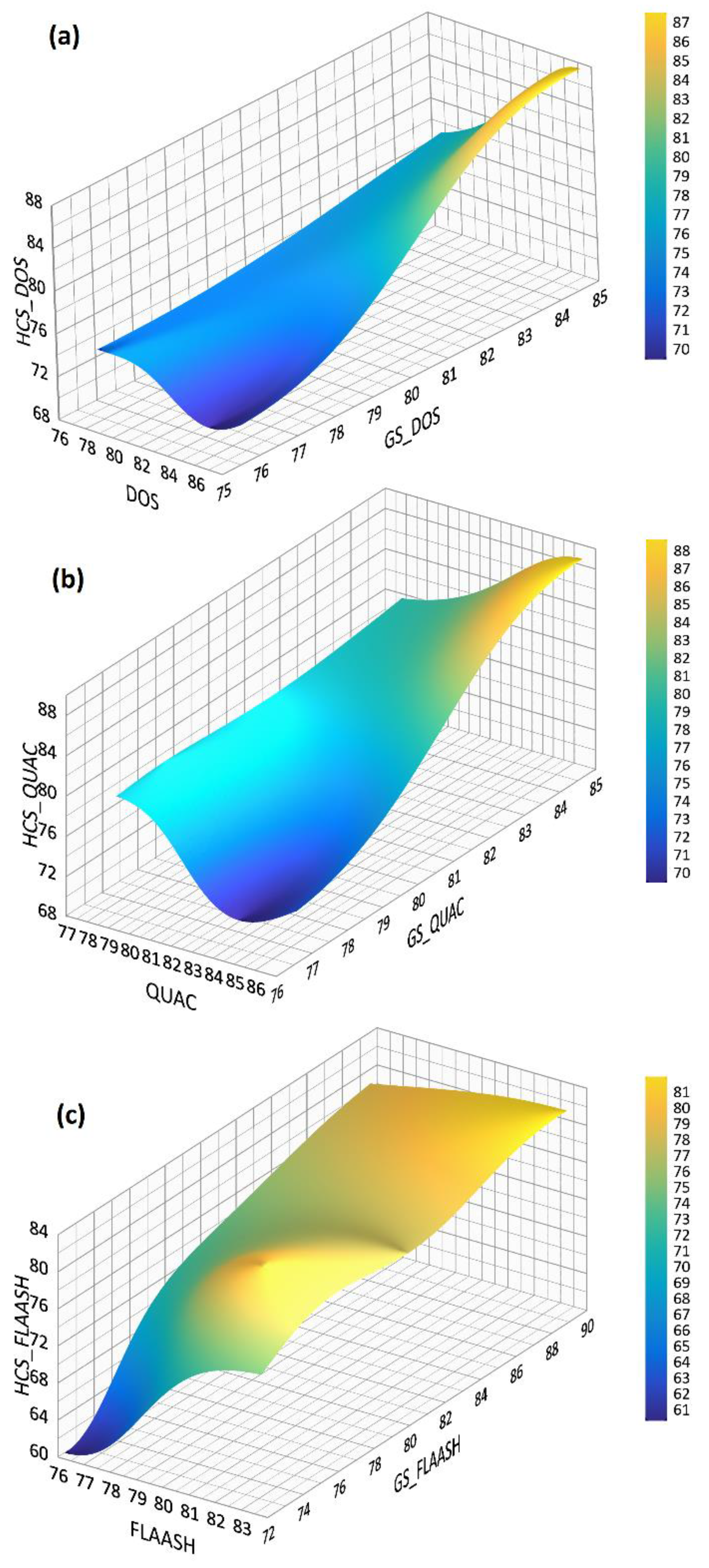
| Rule Sets | DOS | QUAC | FLAASH | GS | HCS | ||||
|---|---|---|---|---|---|---|---|---|---|
| DOS | QUAC | FLAASH | DOS | QUAC | FLAASH | ||||
| Rule Set 1 | 76.67 | 77.78 | 81.11 | 75.84 | 78.34 | 76.11 | 73.33 | 78.62 | 79.85 |
| Rule Set 2 | 84.73 | 83.62 | 76.12 | 75.84 | 76.95 | 72.22 | 69.45 | 69.45 | 60.28 |
| Rule Set 3 | 87.19 | 86.39 | 83.61 | 85.00 | 85.00 | 89.45 | 87.50 | 88.62 | 81.95 |
Publisher’s Note: MDPI stays neutral with regard to jurisdictional claims in published maps and institutional affiliations. |
© 2022 by the authors. Licensee MDPI, Basel, Switzerland. This article is an open access article distributed under the terms and conditions of the Creative Commons Attribution (CC BY) license (https://creativecommons.org/licenses/by/4.0/).
Share and Cite
Jawak, S.D.; Wankhede, S.F.; Luis, A.J.; Balakrishna, K. Effect of Image-Processing Routines on Geographic Object-Based Image Analysis for Mapping Glacier Surface Facies from Svalbard and the Himalayas. Remote Sens. 2022, 14, 4403. https://doi.org/10.3390/rs14174403
Jawak SD, Wankhede SF, Luis AJ, Balakrishna K. Effect of Image-Processing Routines on Geographic Object-Based Image Analysis for Mapping Glacier Surface Facies from Svalbard and the Himalayas. Remote Sensing. 2022; 14(17):4403. https://doi.org/10.3390/rs14174403
Chicago/Turabian StyleJawak, Shridhar D., Sagar F. Wankhede, Alvarinho J. Luis, and Keshava Balakrishna. 2022. "Effect of Image-Processing Routines on Geographic Object-Based Image Analysis for Mapping Glacier Surface Facies from Svalbard and the Himalayas" Remote Sensing 14, no. 17: 4403. https://doi.org/10.3390/rs14174403
APA StyleJawak, S. D., Wankhede, S. F., Luis, A. J., & Balakrishna, K. (2022). Effect of Image-Processing Routines on Geographic Object-Based Image Analysis for Mapping Glacier Surface Facies from Svalbard and the Himalayas. Remote Sensing, 14(17), 4403. https://doi.org/10.3390/rs14174403


