Article

Towards Forecasting Future Snow Cover Dynamics in the European Alps—The Potential of Long Optical Remote-Sensing Time Series

1
German Remote Sensing Data Center (DFD), German Aerospace Center (DLR), Muenchener Strasse 20, D-82234 Wessling, Germany
2
Department of Computer Science, University of Wuerzburg, Am Hubland, D-97074 Wuerzburg, Germany
3
Department of Remote Sensing, Institute of Geography and Geology, University of Wuerzburg, Am Hubland, D-97074 Wuerzburg, Germany
*
Author to whom correspondence should be addressed.
Remote Sens. 2022, 14(18), 4461; https://doi.org/10.3390/rs14184461
Submission received: 18 July 2022 / Revised: 4 September 2022 / Accepted: 6 September 2022 / Published: 7 September 2022
(This article belongs to the Section Environmental Remote Sensing)

Abstract

:
Snow is a vital environmental parameter and dynamically responsive to climate change, particularly in mountainous regions. Snow cover can be monitored at variable spatial scales using Earth Observation (EO) data. Long-lasting remote sensing missions enable the generation of multi-decadal time series and thus the detection of long-term trends. However, there have been few attempts to use these to model future snow cover dynamics. In this study, we, therefore, explore the potential of such time series to forecast the Snow Line Elevation (SLE) in the European Alps. We generate monthly SLE time series from the entire Landsat archive (1985–2021) in 43 Alpine catchments. Positive long-term SLE change rates are detected, with the highest rates (5–8 m/y) in the Western and Central Alps. We utilize this SLE dataset to implement and evaluate seven uni-variate time series modeling and forecasting approaches. The best results were achieved by Random Forests, with a Nash–Sutcliffe efficiency (NSE) of 0.79 and a Mean Absolute Error (MAE) of 258 m, Telescope (0.76, 268 m), and seasonal ARIMA (0.75, 270 m). Since the model performance varies strongly with the input data, we developed a combined forecast based on the best-performing methods in each catchment. This approach was then used to forecast the SLE for the years 2022–2029. In the majority of the catchments, the shift of the forecast median SLE level retained the sign of the long-term trend. In cases where a deviating SLE dynamic is forecast, a discussion based on the unique properties of the catchment and past SLE dynamics is required. In the future, we expect major improvements in our SLE forecasting efforts by including external predictor variables in a multi-variate modeling approach.

1. Introduction

Snow plays a vital environmental, societal, and economic role in many regions around the globe. At the same time, mountainous regions such as the European Alps are highly vulnerable to the effects of climate change. Here, snow cover has a direct impact on the climate system due to its high albedo [1], and the resulting feedback mechanisms are expected to amplify warming at mid to high altitudes [2,3,4,5]. Moreover, snow strongly influences habitats and thus ensures biodiversity. Snow cover duration, for example, proves to be a strong predictor for spatial species distribution [6], while the timing of snowmelt influences plant phenology and productivity [7,8]; thus, climate-change-induced snow cover dynamics also result in habitat shifts and, again, temperature rise due to increased greening effects [4,5]. At the same time, mountains are often described as the water towers of the world, and high-altitude snow cover is a major source of freshwater for billions of people, enabling agriculture and electricity generation [9]. Finally, particularly in the European Alps, snow is the basis for the tourism-based economies of many regions in Austria, Germany, France, Italy, and Switzerland [4,10]. Declining snow cover durations [11] and a continuously receding snow line elevation (SLE) [12] may have severe impacts on Alpine ski tourism in the winter months [10,13,14].
Reliable estimations of future snow cover and SLE dynamics are, therefore, of the highest importance for policy and decision makers, planners, tourism agencies, and other stakeholders in the affected regions (Figure 1). Continuous, long-term, and large-scale ground-based data collection on snow cover dynamics, however, is particularly difficult in fragmented and inaccessible high-altitude mountain areas. Spaceborne Earth Observation (EO) plays a key role in the acquisition of environmental data both at large spatial scales and over long periods of time. For example, Remote Sensing (RS) missions such as Landsat have continuously been acquiring global imagery of the land surface for almost 40 years [15]. Since the inception of the first EO satellites in the 1970s, the archives of RS data have increased dramatically for a number of reasons: a multitude of sensors with different spatial, temporal, and spectral properties has been launched during the last decade that produced a continuous stream of global data; ongoing EO missions have been expanded to enable continuous observations over decades; an increasing variety of analysis-ready (ARD) products has been generated that facilitate scientific analysis of derived geophysical parameters, indices, and thematic information [16]. These developments have been accompanied by rapid advances in computer and data science in the past years. For example, cloud storage and computing have lowered the bar to access and process large EO datasets [17], while newly developed machine learning (ML) methods, especially artificial intelligence (AI), enable unprecedented data-driven insight [18].
These developments facilitate the generation of land surface data products from long RS time series. For example, the Global Snow Pack (GSP) developed by Dietz et al. [19] is a global MODIS-based daily snow cover product enabling snow cover analyses at a 500 m resolution starting in the year 2000. Even longer time series of snow cover dynamics have been generated on the basis of data from the Advanced Very High-Resolution Radiometer (AVHRR) [20,21,22,23]. Both sensors offer very high temporal resolutions, which makes them particularly suitable for the analysis of snow-related climatology and phenology. A very promising technology for snow cover monitoring is Synthetic Aperture Radar (SAR) since its sensing abilities are independent of cloud cover and illumination conditions. This makes SAR data predestined for the generation of gap-free time series. In addition, its ability to detect wet snow facilitates the analysis of seasonal snow-melt onset [24,25]. However, there are no single-sensor SAR products yet available that span several decades, and the continuation of missions such as Sentinel-1 will be invaluable in the future to generate long time series. With Landsat, in contrast, the generation of optical time series starting in the year 1984 is possible. Even though the temporal resolution of these data is lower (16 days) than that of MODIS or AVHRR products, its much higher spatial resolution enables detailed snow mapping even in the complex terrain of high mountain ranges. From datasets such as these, snow cover dynamics can be analyzed over long periods of time, which allows the detection and quantification of long-term trends. Hu et al. [12,26,27] used Landsat and Sentinel-2 multispectral data to retrieve the SLE for select mountainous areas in Europe between 1984 and 2018 at a high spatial resolution. For six catchments in the Alps, long-term linear trends of SLE during the ablation season were also calculated and a significant retreat of the SLE to higher elevations was detected in five cases [12]. Even though this example demonstrates that the detection of long-term trends of land surface dynamics from EO data is possible, the potential of long EO time series for forecasting future processes has not yet been fully utilized [16]. EO time series from missions such as Landsat encompass hundreds of approximately bi-weekly observations over several decades. While Bormann et al. [28] pointed out the limited potential of remote sensing data (namely, MODIS) to quantify long-term trends of snow cover in mountain areas, for now, we argue that the Landsat time series data offers the potential to apply auto-regressive time series models to generate spatially and temporally explicit forecasts for a medium forecast horizon (up to 10 years).
Projections of future snow cover are currently mostly generated from General Circulation Models (GCM) or Regional Climate Models (RCM) at a relatively coarse spatial resolution [4]. In addition, snow cover projections in the European Alps have focused on parameters such as depth or snow water equivalent (SWE) instead of the spatially explicit modeling of snow cover dynamics [4,29,30]. Consequently, we propose closing this research gap by employing long RS time series to analyze past snow cover dynamics and trends and project these into the future. While these forecasts might not (yet) be as accurate as the results from the abovementioned physical models, they are achieved much more easily due to their reduced complexity, especially when generated from ARD, and may give a general indication of future dynamics on variable spatial scales.
Therefore, it is the research goal of this study to assess the potential of long EO time series to model future snow cover dynamics in the Alps. We parametrize snow cover dynamics as the spatio-temporal dynamics of the SLE within a catchment. In pursuit of the research goal, we formulate the following research objectives:
  • Derive multi-decadal time series of SLE dynamics from Landsat data starting 1985,
  • Identify, implement, and evaluate forecast algorithms that can process long EO-based time series data utilizing the generated SLE dataset,
  • Produce actual SLE forecasts for the entire Alps and compare the results to existing climate and snow cover projections.
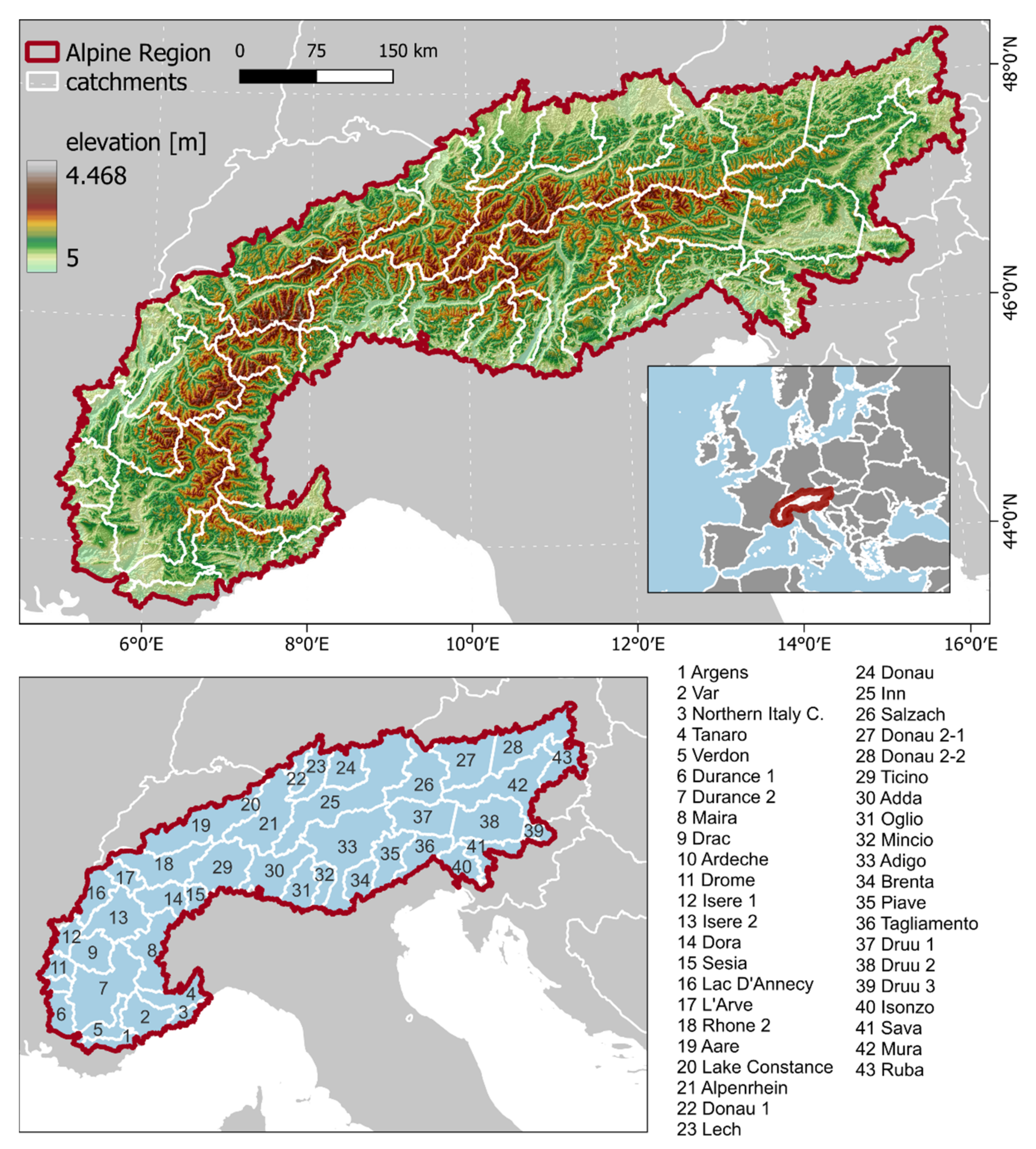
To this end, we adapt and modify an existing algorithm developed by Hu et al. [12,26,27] to retrieve the SLE time series for 43 river catchments from snow classifications generated from Landsat surface reflectance data and a digital elevation model (DEM). We model and forecast these time series using a number of different univariate forecasting techniques and systematically assess the performance of these methods on a test dataset. Using the results of the best performing models in a weighted average approach, we forecast the SLE up to the year 2029 and discuss the results considering recent and projected climate trends in the Alps.
This paper is structured as follows: Section 2 introduces the Alpine region as a study area in which our approach is developed and tested (Figure 2). In Section 3, the data used and the methods applied are introduced. More specifically, the workflow of this study is presented by introducing the snow classification approach, detailing the process of SLE retrieval and time series generation, briefly characterizing the forecasting methods applied, and finally, by outlining the method evaluation and the actual forecasting approach. The results are presented in Section 4 and discussed with respect to the study goals in Section 5. Our findings are summarized in Section 6, where we also give an outlook on future research directions.

2. Study Area

SLE time series were derived for all hydrological catchments within the Alpine region as defined by the Alpine Convention [31] (Figure 2). Within this area, 43 catchments were analyzed. Small parts of larger catchments that intersect with the perimeter were excluded from the analysis. The catchments of the rivers Danube and Drava (Druu) were split into two and three sub-catchments, respectively, since they are covered by multiple satellite acquisition tracks.

3. Materials and Methods

SLE time series were derived for 43 Alpine catchments from Landsat data between 1984 and 2021. The information retrieval is based on the work of Hu et al. [12,26,27], whose approach has been modified to facilitate upscaling of the workflow to larger spatial scales. The SLE observations were filtered for reliability, resampled to a monthly mean and data gaps interpolated linearly to yield an evenly spaced time series of monthly observations. The time series were split in an 80:20 fashion into training and test data. Seven different time-series models were fitted to the training data and their forecast performance was assessed and compared using the test data. According to the “No-Free-Lunch Theorem” [32], we expect that there is no single method that works best for all possible scenarios. Therefore, a combined forecast was generated from the best-performing methods in each catchment by weighted averaging. The combined forecast was evaluated as well and used for actual SLE forecasting up to the year 2029. The workflow is depicted in Figure 3. The data and methods applied are discussed in more detail in the following subsections.

3.1. Data

To generate long time series of SLE observations, data from the spaceborne Landsat sensor family were selected. Its main advantage is the long continuity of regular and comparable acquisitions starting from 1984. Landsat satellites have a revisit time of 16 days with an increased temporal resolution in times where multiple Landsat sensors are operational. This enables the detailed observation of intra-annual dynamics. The spatial resolution is up to 30 m, allowing the detailed mapping of land surface features even in fragmented mountainous regions. Next to the spectral bands in the visible light, near-infrared, and short-wave infrared, Landsat offers a thermal sensor at a resolution of 60 m which is especially useful for the separation of snow and clouds [33].
In order to save processing time and effort, Landsat Collection 2 Level-2 Tier 1 Surface Reflectance (SR) data were used. These products provide already atmospherically and topographically corrected reflectance values that are comparable across different Landsat sensors and thus enable time series analysis [34,35,36]. We acquired data from 19 Landsat tiles covering the acquisition paths 190 to 196 and rows 26 to 30. Using all available imagery of these tiles, 14,526 scenes were processed. Between ~800 and ~900 scenes were available for each tile, with increased data coverage in more recent years, where multiple sensors were operational simultaneously. Using passive optical sensors, Landsat imagery is prone to obstruction by clouds and scenes with a high percentage of cloud cover can often not meet the Tier 1 quality standard. As a result, there are fewer data available in the winter months than in summer; however, we refrained from the a priori exclusion of data based on an arbitrary threshold of cloud cover percentage, since the SLE is derived on a catchment basis which is only a subset of the entire scene and may contain fewer clouds. Furthermore, as a statistical measure, the SLE can be estimated on a relatively small subset of the data, albeit with reduced reliability (c.f. Section 3.3).
The Copernicus Global and European Digital Elevation Model were used for the retrieval of the elevation of the snow line from the Landsat-based snow classification images. We used the GLO-30 variant, which has a spatial resolution of one arc-second, matching the 30 m resolution of Landsat data [37]. Due to snow being an important hydrological parameter, we chose river catchments as the spatial unit of analysis for which the SLE is calculated. We used the HydroBASINS dataset of the HydroSHEDS project, a database of vector files containing the boundaries of river catchments and their sub-catchments at a 15 arc-seconds resolution [38].

3.2. Snow Classification

As proposed by Hu et al. [12,26,27], we employ a threshold-based snow classification scheme. It combines a temperature and shadow thresholding developed for the Satellite Snow Product Intercomparison and Evaluation Exercise (SnowPEx) [39] and a follow-up index-based thresholding scheme originally designed for MODIS data [40,41,42]. In this approach, potential snow pixels are identified in a decision tree which checks for thresholds in the green and near-infrared (NIR) spectral bands, as well as the spectral indices, normalized difference snow index (NDSI) [43], and the normalized difference vegetation index (NDVI) [41,44]. Several masks are then applied to the resulting snow classification: A temperature mask greater than 288 K rules out pixels with a temperature too high for the occurrence of snow, a threshold combination of the normalized difference water index (NDWI > 0) [45] and reflectance in the visible green band (<0.2) delineates water bodies, and a combination of low values in the short-wave infrared (SWIR, <0.02), green (<0.2), and NDVI (<0.1) refers to topographical shadow. Finally, a cloud mask based on the FMASK algorithm is applied [46].
This approach was modified to match the requirements of Landsat SR data. The binary cloud mask necessary for this approach was generated from the pixel quality bands (PIXEL_QA) provided with the SR data. The NDSI, which is calculated from the green and SWIR bands, has a particularly important role in snow classifications but also limitations under certain conditions. For example, it has been shown that the static standard threshold of the NDSI of 0.4 is insufficient for snow classifications at a local scale [47]. Moreover, the suitability of the NDSI for snow detection is influenced by variable local illumination conditions due to topography [48] as well as the occurrence of bare rock [49]. Therefore, we introduced a normalized difference between the blue and NIR bands to the classification scheme, which uses the high reflectance of snow in the visible blue and the low reflectance in the NIR bands. When differenced with the NDSI, the new index can help distinguish snow from sunlit rock, bare soil, water, and clouds. The resulting classification encompasses the classes “clear land”, “snow”, “clouds”, “water/shadow”, and “no data”. The accuracy of the classification scheme has been assessed using validation polygons on Landsat, Sentinel-2 imagery as well as the Google Satellite Base Map in Google Earth Engine. Then, 5000 to 6000 point samples within these polygons from two classifications of each Landsat sensor type were taken for each class in a stratified sampling approach and compared to the ground-truth data in a confusion matrix. For the following SLE retrieval, the classes “clear land” and “snow” are the most relevant, whereas confusion between the remaining classes has no influence on the SLE estimation accuracy. Therefore, “clouds”, “water/shadow”, and “no data” were summarized into a single “invalid” class for the accuracy assessment. On average, the classification of the Landsat 5 data (sensor ETM) achieved an overall accuracy of 87.5%, Landsat 7 (ETM+) of 95.5%, and Landsat 8 (OLI) of 94.5%. Confusion results especially from clouds close to or over snow-covered mountain tops.

3.3. Snow Line Elevation Retrieval and Time Series Generation

Using the snow classification and the Copernicus DEM, the SLE was calculated for each Landsat observation on a catchment basis. We applied an approach originally developed by Krajčí et al. [50], who derived the SLE for a catchment in the Carpathian Mountains from daily MODIS data for the period 2000–2013. Krajčí et al. parametrized the (regional) SLE as the elevation for which the sum of snow-covered pixels below and land pixels above can be minimized. The derived SLEs were validated using in-situ snow measurements from climate stations achieving an average accuracy of 86% [50]. This approach was transferred to the Alps and Landsat data by Hu et al. [26], who described the SLE as a statistical measure that can be calculated as the minimum of the sum of the two cumulative histograms of “snow” and “clear land” pixels over the elevation. As a result, it is possible, to a certain degree, to estimate the SLE even in clouded conditions if enough sample pixels are available [50]. Figure 4 shows a quick overview of the process of deriving the SLE from a satellite image. To evaluate the accuracy and the reliability of the SLE estimation, several quality indices are calculated for each derived SLE. We employ the Representativeness Index (RI) to evaluate how many valid pixels (i.e., “snow” and “clear land”) have been available for the SLE estimation. The Root Mean Square Error (RMSE) gives a measure of the accuracy of the derived snow line by calculating the distance of falsely classified pixels (i.e., “snow” below the SLE, “clear land” above the SLE) from the estimated SLE. The share of these erroneous pixels is calculated with the Error Index (EI) [26].
For the following time-series analysis, a time series with a regular observation frequency is required. In the first step, we filtered the derived SLEs based on their quality. We rejected SLEs derived from images with an RI < 0.2, as well as SLEs outside the elevation range of each catchment as derived from the DEM. Depending on the catchment, between ~64% and ~89% of all observations remained. Afterwards, the remaining observations were aggregated to monthly mean values to produce a regular time series. The remaining data gaps were filled using linear interpolation. More sophisticated interpolation methods were considered. For example, Hu et al. [12] closed SLE data gaps in a Random Forests regression using external weather and climate variables; however, we wanted to specifically assess the suitability of RS data for time series forecasting and therefore restrict the use of additional data. Problems resulting from linear interpolation are further addressed in the results and discussion sections. Since the intended forecasting methods require full-cycle observations (i.e., entire years), we cropped the time series to start in January 1985 and end in December 2021. This resulted in a time series comprising 444 SLE estimations for each catchment, which are used as the basis for the following model building and forecasting. We applied the two-sided seasonal Mann–Kendall test [51] to determine the significance of any long-term trends within the time series and used the seasonal Theil–Sen estimator [52] to calculate yearly change rates.

3.4. Forecasting Methods

The main goal of this study is to assess the feasibility of EO time series for forecasting and to which degree existing forecasting approaches are capable of achieving that. To this end, seven forecasting approaches were selected to forecast the SLE in two Alpine catchments and their performance was evaluated. We selected these methods, which are introduced below in more detail, for their versatility, their established use in other scientific fields, and because they are easy to apply using existing software packages. Furthermore, a combined forecast is generated from the best performing forecasts in each catchment and then also evaluated. We limited the scope of this study to the use of univariate forecasting methods, as their implementation does not require any additional data other than the original time series that is to be forecast. This means that we use exclusively past observations of the SLE to train and apply the models. Thus, we can evaluate whether and to what degree long time series of EO data can be the base of reliable forecasts of land surface dynamics. We are aware that external climate and meteorological parameters such as temperature or precipitation may be stronger predictors for SLE dynamics than past SLE observations; we discuss this further in Section 5.3. The selected forecasting methods provide a cross-section of different forecasting paradigms employing approaches based on exponential smoothing, auto-regression, machine learning, or a combination of these. All of the methods have been implemented using the statistical programming language R, which offers established libraries for time series analysis and forecasting. The applied methods are introduced briefly in the following paragraphs:
Seasonal Naïve: The simplest form of the forecast is the naïve forecast which sets the forecast value(s) equal to the last observation. We applied the variant seasonal naïve (sNaïve), since the SLE data are highly seasonal. Therefore, in this approach, the forecast value for each month is equal to the value of the corresponding month of the previous year. The results of this forecasting method are merely used as a benchmark for the remaining approaches, which should perform considerably better [53].
ETS: In exponential smoothing forecasting, the forecast value is a weighted average of the previous observations, whereas more recent observations have an exponentially greater weight than old ones. For model fitting, exponential smoothing uses one or multiple components of a time series, whose parameters have to be estimated to build the model. ETS stands for the three components error, trend, and seasonal, which modify the smoothing method of the model. In the ETS implementation of the “forecast” package in R, the ideal model parameters are chosen automatically [54].
Seasonal ARIMA: Autoregressive Integrated Moving Average (ARIMA) models use auto-correlations within the data rather than describing error, trend, and seasonal components such as ETS. The order of an ARIMA model is determined by three components p, q, and d and is denoted as ARIMA(p,d,q), with p being the order of the autoregressive part, d being the number of differencing, and q being the order of the moving average part of the model. If the modeled time series has seasonality, additional components analog to p,d,q of the non-seasonal part are introduced (sARIMA) [53]. In the ARIMA implementation of the “forecast” package in R, the optimal parameter combination is chosen by the application of the automated Hyndman–Khandakhar algorithm [54].
ANN: Artificial Neural Networks (ANN) enable the non-linear modeling of a variable based on multiple predictors and can also be used for time series forecasting. Here, a multi-layer feed-forward neural network with one hidden layer in addition to the input layer is used. The number of neurons in the hidden layer and the number of observations directly prior to the forecast, which are used as predictors, are optimized automatically by the model. We manually set the number of previous years of observations to consider by the ANN to ten to make use of the long history of observations. Multiple forecasts are generated iteratively using the already forecasted values as input for the following ones. Prediction intervals are computed from the distribution of forecast values from 1000 NNAR runs [53].
Random Forests: Random Forests (RF) is a machine learning classification and regression scheme based on decision trees and was developed by Breiman [55]. Since here the forecast values are continuous, an ensemble of regression trees is grown randomly from a sample of the input data that is sampled by bootstrapping (i.e., with replacement). In addition, each tree is built from a random sample of features to avoid overfitting. The results of the regression trees are averaged to yield the forecast value [55,56]. For forecasting the SLE, we build an input matrix of lagged values, where each predicted value is a function of the past twelve observations. The RF-based forecast is then applied iteratively so that forecast values closer to the forecasting horizon are based on already predicted values.
XGBoost: XGBoost is an ML classification and regression framework and is, similar to RF, based on ensembles of classification and regression trees. In XGBoost, the optimization of the loss function is conducted using a gradient boosting approach, where each tree is grown sequentially using the information of the previous trees [56,57]. Similar to the implementation of RF, the XGBoost model is provided with a matrix of lagged values and the forecast is conducted iteratively. In our implementation, the number of boosting rounds is set to 500, which is stopped earlier if there is no significant accuracy gain for 50 iterations.
Telescope: Telescope is a generic hybrid forecasting approach developed by Bauer et al. [58,59]. In an automated framework, Telescope extracts various features from the input time series and forecasts each component using different, appropriate forecasting methods. The final forecast is then composed in a regression-based machine learning algorithm. By default, the applied ML approach is XGBoost. However, Telescope can also apply an elaborate ML model recommendation scheme to select the most appropriate model from a selection of seven different approaches (for more details, c.f. [56]). For convenience, we use the default settings here.
Combined forecast: The results of the best performing forecast results in each catchment are used to generate a combined forecast. For this, only the results of forecast methods are used that reached a Nash–Sutcliffe efficiency (NSE) of 0.6 or higher in the respective catchment. If less than two methods exceed that threshold, only the results of the best performing method are used. In any case, sNaïve was not included in the Combined forecast. The forecast values of the selected forecasts are aggregated using a weighted average with respect to their NSE performance to calculate the final combined forecast result. The prediction intervals for this approach are calculated from the forecast means of the forecasting methods used in the forecast combination.

3.5. Model Evaluation and Forecast

To evaluate the forecasting performance of the methods introduced in Section 3.4 we split the monthly SLE time series for each catchment in an 80:20 fashion. Thus, the observations of the test dataset are independent of the training observations used for building the models [53]. The resulting training datasets comprise observations from 29 years (1985–2013), which is close to the 30 years over which climate normals are recommended to be calculated by the World Meteorological Organization [60] and therefore allow the detection of trends independent of seasonal variation. The results of the evaluation on a test dataset of eight years (2014–2021) are representative of the performance of the actual forecast up to the year 2029 [53]. In total, each monthly time series consists of 348 observations used for model training and 96 observations for model testing.
We evaluate the forecast association using the NSE and the accuracy using the Mean Absolute Error (MAE). The NSE is widely used in hydrology to evaluate the prediction quality of discharge time series but can be transferred to other prediction applications. It is calculated as:
N S E = 1 t = 1 n P t O t 2 t = 1 n O t O ¯   2 ,
where n is the number of time steps, Pt and Ot are the predicted and observed values at time step t, respectively, and Ō is the mean of all observations. Thus, it is calculated by subtracting the ratio of the Mean Squared Error (MSE) and the variance of the observations from 1. It can be interpreted as the skill score of the forecast compared to the mean of the observations. If the NSE < 0, the forecast is less accurate than the mean, with NSE = 1 indicating a perfect score [61,62]. The NSE can be decomposed into three components in a more detailed evaluation approach, i.e., the Kling–Gupta efficiency (KGE). It addresses issues of the NSE arising when comparing forecasts based on highly seasonal time series in regions with different seasonality patterns and in cases where the NSE is used for model optimization [61,63]. Since the SLE seasonality are similar in every catchment and we do not further optimize the models, we used the NSE metric, which is easier to interpret in comparison to the KGE.
While the NSE gives a good indication of the overall model fit, the MAE quantifies how accurate the predicted SLE values are. It is calculated as:
M A E = 1 n   t = 1 n P t O t ,
where n is the number of time steps, and Pt and Ot are the predicted and observed values at time step t, respectively. It can be easily interpreted as the mean deviation of the model from the forecast in meters, and the smaller the result, the better the forecast performance [53,64].
Finally, we used the Combined forecasting approach to forecast SLE values for the years 2022–2029. Thus, we expect a more robust forecast than predictions made based on a single algorithm. The forecasting horizon of eight years reflects the length of the test period the models were evaluated on and can thus be expected to yield a comparable performance. The forecast SLE is compared to prior observations by comparing the level of the median. Furthermore, we use swath profiles of the catchment elevation to discuss the impacts of the forecast SLE dynamics spatially.

4. Results

4.1. Properties of the SLE Time Series and Long-Term Dynamics

The SLE and several corresponding quality measures were derived from each Landsat-based snow classification. Before aggregating and interpolating the results (c.f. Section 3.3) for each catchment, the distributions of the RI, the EI, and the RMSE were explored (Figure 5). Note that the filtered dataset only contains observations with an RI ≥ 0.2. For more than 80% of the estimated SLEs, at least 40% of all pixels in the scene were suitable, with the median RI located at 0.64. The share of falsely classified pixels (i.e., “snow” below the estimated SLE, “clear land” above the SLE) within a catchment was low, with a median EI of 0.006 and the 80th percentile located at 0.027. The median accuracy of the estimated SLE as measured by the RMSE is 255 m, with 80% of the values better than 605 m. The RMSE peak in the first histogram bin is due to a very low RMSE in scenes where very little to no snow is present. High RMSE values, i.e., a low reliability of the SLE estimation, are often associated with a low RI value.
After applying the quality thresholds to the data, between ~64% and ~89% of all observations remained, depending on the catchment. These were used and aggregated on a monthly basis to generate regular, evenly spaced time series. Three examples of monthly SLE time series ranging from 1985–2021 are displayed in Figure 6. Especially in the examples from Rhone and Lech, the time series show the seasonal pattern expected from the SLE, which has the lowest values in the winter months and recedes to higher elevations in summer. The theoretical minimum and maximum SLE are determined by the minimum and maximum elevation in the respective catchment. Since the theoretical minimum (i.e., entire catchment covered in snow) is, in practice, seldom reached, the actual minimum SLE varies strongly between years. In contrast, the SLE actually reaches its theoretical maximum in summer much more often. This is the case particularly in catchments with low to medium elevations, where the catchment is entirely snow-free for multiple consecutive months and there is no physical SLE to be estimated. In the time series data, the SLE is then locked to the highest possible elevation in the catchment and appears to be maxed out. This effect is visible to a certain degree in Lech, but much stronger in Argens. Here, instead of a seasonal sine pattern, snowfall events appear as negative spikes from the median SLE line. This strongly affects the ability to accurately model the SLE time series (c.f. Section 4.2) as well as the detection of a long-term trend in these catchments: While trends with a high significance can be detected in catchments where the SLE maxes out only weakly such as Lech, no trend at all can be detected where the SLE is maxed out strongly such as in Argens. Of the 43 catchments analyzed, 15 showed a medium to a strong degree of a maxed-out SLE. These are treated separately in the discussion of the results.
The map in Figure 6 shows the calculated long-term SLE trends and their statistical significance for all analyzed catchments (also, cf. Table A1). The majority of catchments experienced a significant positive yearly SLE change of between 2 and 8 m/y in the past 37 years, i.e., the SLE is gradually moving to higher elevations. These trends are especially pronounced in the Western and Central Alps. Here, Drac (8.92 m/y), Upper Durance (7.28), Adigo (6.92), Adda (6.65), and Inn (6.25) exhibit the strongest trends. Negative SLE trends are present especially in the Eastern Alps in Mura (−2.00 m/y), Central Drava (−1.09), Sava (−0.89), and Isonzo (−0.40), as well as the South-Western Alps in Tanaro (−0.04) but at a much lower magnitude and less significance. The effect of a maxed-out SLE in the summer months is visible on the outer fringes of the Alps, where catchments exhibit very weak and statistically insignificant trends.

4.2. Evaluation of Forecasting Approaches

Based on the 348 observations of the training data (1985–2013) in each catchment, seven models were trained and forecasts were conducted for the following eight years (2014–2021). The resulting forecast time series comprised 96 forecast values each, which were validated using the test data set.
Figure 7 shows the performance of each forecasting method as measured by the NSE in each catchment where the SLE is not maxed out (left) and those where it is (right). A high NSE score throughout is achieved by Telescope, RF, and the Combined forecast in catchments where the SLE is not maxed out. Here, also sARIMA and ANN performed satisfactorily. ETS, sNaive, and XGBoost, in contrast, performed especially weakly in a few catchments where the mean of the observations would be a better forecast (NSE < 0). The overall forecast performance is lower in catchments with a maxed-out SLE. Here, no method achieves an NSE > 0.8 in any catchment, and for Argens and the lower Druu catchment, the NSE is below zero for most of the forecasting approaches. In snow-free catchments, the forecast quality apparently depends on the input data rather than on the selected method. However, RF, Telescope, and the Combined forecast appear to be somewhat robust to difficult time series patterns.
The superior performance of the forecast methods in non-maxed-out catchments also shows when the NSE is aggregated over all catchments (Figure 8). The median forecast association is considerably higher in these catchments with much less variance. The highest median NSE is achieved by the Combined forecast (0.79) and RF (0.79), followed by Telescope (0.76). Forecasts for snow-free catchments, in contrast, are much less reliable and the median NSE is considerably lower. Outliers produced by some forecasting approaches can be mitigated by using the Combined forecast, while at the same time reaching a comparably high median NSE of 0.63. However, single negative outliers such as the Argens catchment remain even in this approach.
The MAE was used to quantify how accurately the SLE is forecast by each evaluated method in each catchment (Figure 9). For catchments in which the SLE does not max out in the summer months, in most of the cases, an MAE between 200 and 400 m is achieved, with outliers in both directions. Here, the Combined Forecast (median MAE: 256 m), RF (258), Telescope (268), and sARIMA (270) perform best on average (Figure 10). In particular, ETS and XGBoost have greater outliers in single catchments and are less reliable. The best forecast overall is achieved by the Combined forecast with an MAE of 178 m in the Adda catchment. In contrast to the NSE, the forecast performance appears to be better in catchments with a maxed-out SLE when measured by the MAE. Here, 58% of all forecasts made achieve an MAE < 200 m. The best forecast is achieved by RF in Ardeche with an MAE of 72 m and there are no extreme outliers. In contrast to the catchments showing summer snow, in snow-free catchments, the forecast performance is more dependent on the input data than on the applied forecasting method. We attribute the better MAE performance to the fact that large SLE outliers that diverge from the forecast median occur less often in maxed-out catchments and are smaller in magnitude due to the less pronounced topography.
Furthermore, the general fit of the forecast time series compared to the observations was assessed qualitatively by visual comparison. Figure 11 shows an example of the forecast results generated by the eight methods for the catchment Drac. Drac is located in the Western Alps, exhibits a strong positive SLE trend of 8.9 m/y, and there is no maxing-out of the SLE in summer. Here, the tested forecasting methods achieve high NSEs and low MAEs throughout, with the exception of XGBoost (c.f. Figure 7 and Figure 9). This example shows that most of the forecasting methods are able to model the seasonal variation in timing and amplitude quite well. Naturally, there are inaccuracies where extreme SLE values (e.g., the SLE minimum in winter 2017/18) or deviations from the seasonal patterns occur (snow melt and intermediate snowfall event in winter 2016/17). Nonetheless, in Drac, all methods except XGBoost achieved a high NSE over 0.6 and could be used for the Combined forecast, which achieved an NSE of 0.81 and an MAE of 303 m. A significantly weaker performance of XGBoost can also be observed in other catchments with a high SLE variance, such as Lech, Lac D’Annecy, and Oglio. XGBoost is known for its strength in modeling time series with a vast amount of input data, while the number of observations in the SLE time series is comparably low, which could serve as an explanation for this unreliable forecast behavior; however, in catchments with a lower variance and only singular outliers, such as Adda and Isere 2, XGBoost yields better results.
The coast of Northern Italy is an example of a catchment, in which the SLE maxes out for several months in summer and which yields very diverse forecasting results (Figure 12). sARIMA, for example, stops modeling a seasonal pattern after the second forecast year and rather estimates a mean SLE. Actually, this still results in a good MAE of 192 m, but at the same time, the NSE is low at 0.19, indicating only a slight improvement over an entire mean forecast. ANN matches the observations well up to the year 2018 but then strongly over- or underestimates the following four winter seasons, resulting in a negative NSE. The winter SLE descent is forecast much more conservatively by XGBoost, which results in less deviation from the extreme values in 2018 to 2021 and a much better NSE (0.47). In this catchment, where no single method exceeds the NSE threshold of 0.6, XGBoost is the best performing algorithm and thus the only input to the Combined forecast.

4.3. Forecast of Future Snow Line Elevation in the Alps

In the next step, all methods were trained on the entire SLE time series (1985–2021) in each catchment and forecasts were conducted up to the year 2029 based on the newly fitted models. Since there is no validation possible for the actual forecast, the Combined forecast was calculated using the methods that exceeded the 0.6 NSE threshold in the evaluation based on the test dataset. Forecasts were generated only for catchments in which the SLE does not max out because only those are reliable. Figure 13 shows three examples of the forecast time series as generated by the combined forecast in comparison to the observations from 1985–2021. In the forecast evaluation, Mincio and Adda achieved good results both in NSE and MAE. This can be attributed to the low variation in the observation time series (grey), with only small outliers beyond the 20th and 80th percentiles. As a result, the forecast (red) matches the observations well both in pattern and amplitude. Both Mincio (5.7 m/y) and Adda (6.6 m/y) exhibit a positive long-term SLE trend, and thus the resulting median SLE is higher for the forecast time series than for the observed time series (Mincio +16 m, Adda +55 m). Even though a positive long-term trend was also detected for the Drac catchment, the median SLE of the forecast is lower than the median of the observations (−74 m). Here, the amplitudes of the outliers in the observation time series are much higher and positive and negative extreme values occur much more frequently than in the other two example catchments. Even though the forecast does not predict an increased median SLE, the intra-annual SLE variance is expected to increase, as indicated by the wider margin between the 20th and 80th percentiles of the forecast compared to the observations.
The difference between the medians of the observed and the forecast time series was further analyzed for all catchments in the Alps (Figure 14, Table A1). This metric gives an indication if the SLE is projected to retreat to higher (positive difference) or descent to lower elevations (negative difference). However, a positive long-term SLE trend does not necessarily result in a positive median SLE difference, as the example from Drac shows in Figure 13. 17 of the 28 catchments (61%) in which the forecast up to 2029 was conducted retained the sign of the long-term trend in the median difference. Possible reasons for that are further addressed in the discussion (Section 5.3). With the exception of Drac, catchments with a strong positive SLE trend (>6 m/y) also have a positive median difference, i.e., the median SLE is forecast to recede to higher elevations in the future. Furthermore, there are two clusters of catchments with a negative difference in medians while the long-term trend was positive. In the Eastern Alps, the catchments Upper Drava, Piave, and Brenta exhibit a weak long-term trend of ~+2 m/y. Similar to the example of Drac, the observed times series in these catchments exhibit frequent SLE outliers beyond the 20th and 80th percentile. The resulting forecast median and percentiles are well below the observations here. In the Western Alps L’Arve, Dora, Sesia, and Maira have stronger positive trends around +4 to +6 m/y, while the negative median shift is smaller than in the Eastern Alps. The details in Figure 13 show the location of the median, 20th, and 80th percentile of the forecast SLE in comparison to the long-term observations in the topography of the catchments Adda and Mura. In Adda, the shift of the 80th percentile is much stronger than that of the 20th percentile, indicating that the retreat of the SLE in summer is more pronounced than in winter. In Mura, in contrast, the median SLE is forecast to move to lower elevations in the coming years, while the winter SLE stays relatively stable.
The actual effect of changing SLE dynamics in each catchment strongly depends on its unique topography and elevation distribution. To better illustrate this, swath profiles from west to east were generated for each catchment. These show the elevation distribution of the terrain for each north–south transect using the maximum, median, and 80th elevation percentile. By mapping observed and modeled SLE key metrics into the swath profile, the effects of a changing SLE in the future can be analyzed for the respective catchment (Figure 15 and Figure A1).
For example, the swath profile of the upper Durance catchment in the Western Alps shows that especially the eastern part of the catchment is directly affected by changing SLE dynamics, while in the west, more than 80% of the elevation lies below the 20th SLE percentile. The projected median shift of +69 m thus affects particularly the upper reaches of the catchment. Here, we highlighted the elevations that are covered in snow at least 50% of the time, i.e., the area above the SLE medians, which is projected to substantially reduce in the coming years. While in Durance, an overall shift of the SLE to higher elevations is forecast in all seasons, future seasonal SLE dynamics are more ambiguous in Drac. The negative median difference (−74 m) is accompanied by an increased level of the 80th percentile and a decrease in the 20th percentile of the SLE. Both percentile levels are associated with the SLE in the summer and winter seasons, respectively; therefore, in winter, the SLE is projected to reach lower elevations more often, while in summer, it will retreat to even higher elevations than before.

5. Discussion

5.1. Forecasting Alpine SLE from Long EO Time Series

To detect, model, and forecast trends of land surface dynamics at a large and continuous scale, EO missions that have been operational for several decades are required. The generation of long EO time series has only been possible for a few years since Landsat entered its fourth decade of operation. As a result, the potential of these time series to forecast land surface parameters such as snow cover dynamics has not yet been fully utilized [16]. In this study, we modeled future SLE dynamics in the Alps by training and evaluating well-established univariate forecasting models on long time series of freely available Landsat data. Even though the sensors and products of the Landsat mission have been harmonized with regards to their spatial, temporal, and spectral properties, generating a long time series of a geophysical parameter such as the SLE remains a challenge. Compared to the original framework by Hu et al. [12,26,27], in this study, we streamlined the time series generation process by using SR data instead of performing the atmospheric correction ourselves; however, it was still necessary to download, classify, and retrieve the SLE from the entire Landsat archive since 1985. Moreover, to generate a regular time series that can be used in time series modeling, additional preprocessing steps such as filtering, and interpolation were still required. This highlights the need for further EO ARD products, from which scientific analyses can be performed more efficiently.
Nonetheless, we were able to generate an SLE time series of 37 years for each Alpine catchment, which enables the characterization of seasonal as well as long-term SLE dynamics. The goal of this study was to model these time series in order to be able to forecast future SLE dynamics. We opted for a univariate time series forecasting approach solely based on past SLE observations to assess the degree to which EO time series data are able to forecast spatio-temporal land surface dynamics. Since there has been little research on univariate forecasting from long EO time series until now, we compared seven forecasting methods in order to identify the most appropriate approach regarding the particularities of long EO time series.
In contrast to bivariate or multivariate approaches, which utilize one or multiple predictor variables to model a dependent variable by regression, univariate modeling relies exclusively on the temporal patterns of past observations to model future values. Well-pronounced regular seasonal patterns and strong trends will enable the algorithm to reliably model the time series and predict future values. These patterns were visible in the majority of the SLE time series we derived from EO data and thus the respective test forecasts achieved a high NSE and a low MAE (Figure 7 and Figure 9). However, frequent and strong outliers from these regular patterns deteriorate the model performance, as is evident when comparing the relatively regular time series of Adda with the more variable SLE dynamics in Drac (Figure 13), which resulted in quite different NSE and MAE values (Figure 7 and Figure 9). The extreme case occurs in catchments where no snow cover is present for multiple months in summer. Here, instead of forming a seasonal sine pattern, the SLE baseline is locked at the highest possible elevation in the catchment and snowfall events appear as singular extreme outliers from said baseline. Without this regular pattern, univariate time series modeling approaches have great difficulties in accurately modeling these dynamics. As a result, we found that the quality of an SLE time series model depends on the input data rather than on the modeling algorithm. In accordance with the “No-Free-Lunch Theorem” introduced in Section 3, there is no single method that performs equally well under all circumstances.
Similarly, the forecast performance varied considerably between the evaluated methods, even within the same catchment. For example, the ML methods RF, ANN, and XGBoost show variable performances across all time series. ML modeling usually profits from a high volume and variety of input data. In the case of the SLE time series, however, the training data are limited to a few hundred numerical observations. Evidently, of these three methods, RF is best suited to deal with the limited amount of input data and still predicted the SLE reliably in catchments with summer snow. Moreover, RF appears to be less reliant on regular seasonal patterns than the classical time series models sARIMA and ETS and achieved relatively good results even in difficult scenarios with a maxed-out summer SLE. In contrast, the performance of XGBoost varied considerably. In some cases, it yielded excellent results compared to the other methods (catchments Isere 2, Isonzo), while in others, such as Drac, it performed considerably worse. By design, XGBoost is optimized to generate predictions quickly and from a vast amount of input data, and apparently struggles with a limited amount of highly variable data. After the models were calibrated on the historical SLE data, we generated the forecasts of the ML methods iteratively using the twelve observations prior to the predicted value (cf. Section 3.4). To improve the forecasting results, a systematic hyperparameter tuning of each method could be performed, which was beyond the scope of this study. Such an assessment could reveal if there is an optimal set of parameters enabling the reliable prediction of all time series scenarios or whether these parameters have to be fit to specific time series patterns. In comparison to the automated parameter selection of ETS or sARIMA, this makes the optimized use of the ML methods quite work intensive. On the other hand, ML offers the potential to easily add predictor variables for multivariate modeling approaches in the future.
The implementation of ETS, sARIMA, sNaïve, and Telescope was quite straightforward in comparison. However, sARIMA was much more reliable than ETS in modeling SLE in the scenarios where the SLE is not maxed out and yielded solid results throughout. Being more reliant on recurring patterns, sARIMA’s performance deteriorated more than, for example, that of RF, XGBoost, and ETS when the SLE maxed out. As expected, sNaïve had the weakest performance overall. Since it simply repeats the pattern of the last season, good forecasting results are only to be expected if said season is representative of the general seasonal pattern. While in some singular cases, this can be a solid approximation, in general, it is worthwhile to invest some extra effort into building a more sophisticated forecasting model.
The fact that no forecasting model performs equally well in all scenarios implies that a hybrid approach combining multiple forecasting methods may result in a more robust forecast. This assumption is supported by the overall good performance of Telescope, which applies different modeling approaches for different components of the time series (cf. Section 3.4). Alongside RF, Telescope achieves good forecast results throughout with only a few negative outliers (e.g., in Upper Danube and Verdon) and is, at the same time, easy to implement. Considering this, we developed the Combined forecasting approach, which dynamically selects and averages the best forecast results for each time series. Thus, we were able to minimize the variance across multiple time series and make the forecast more robust to difficult SLE scenarios. Consequently, the Combined forecast scheme achieved the best forecast results throughout.

5.2. Model Reliability and Error Sources

Models are simplified versions of phenomena and processes of the real world and thus are never completely accurate. Forecasts are the last link in a chain of numerous instances of data processing, assumptions, and model building. Even if a forecast is technically feasible, it is always subject to uncertainties and errors that are introduced with each step of approximation or simplification. It is, therefore, good practice to make potential error sources in the generation process of the forecast transparent.
In this regard, the first issue to address is the accuracy of the SLE estimation, i.e., the input time series. The basis for the SLE estimation is the snow classification for each single Landsat scene. For this, a very simple and highly accurate classification scheme was used as proposed by Hu et al. [12,26,27], which we further improved to better discriminate snow spectrally. From this, for each scene and catchment, the SLE was calculated. At this point, it is important to note that the SLE is not a real physical entity in the form of a sharp boundary line that can be directly extracted from the EO images. Instead, it is a statistic calculated from the spatial distribution of “snow” and “snow-free” pixels across the catchment and its topography. It thus has a certain fuzziness that is expressed by the distance of “snow” pixels below and “no-snow” pixels above the estimated line. The actual location of the SLE can, therefore, not be validated in the field since it lacks its real physical counterpart. Instead, the reliability of its estimation is quantified by how many pixels have been available for its estimation (measured by the RI) and the abovementioned fuzziness (RMSE). For this reason, an RI-based quality thresholding was applied prior to the generation of the final time series.
The mathematical modeling of the SLE in a time series requires a regular, evenly spaced time series with a fixed frequency. In reality, the derived SLE observations are unevenly distributed across time as a result of both the number of available satellites and obstruction due to cloud cover; therefore, the observations were aggregated by calculating the monthly mean. Using the median was considered, but we did not want to smooth out extreme values that were observed in reality, even if it would have been easier to model such a time series in the following steps. Furthermore, remaining data gaps in months in which no SLE estimation was available were closed through linear interpolation between the temporally neighboring observations. In that regard, we expect major improvements, especially for longer data gaps, as a result of the introduction of predictor variables, which will enable the modeling of missing values on a physical basis and even facilitate the generation of a denser time series. For the time being, however, the generation of the regular SLE time series from the observations is a further modeling step that may influence the final forecast results.
However, for the overall forecast quality, the performance of the applied time series model is of the greatest importance. Errors at this step can be and have been quantified and extensively analyzed. The strengths of the univariate approaches evaluated in this study lie in the detection and modeling of recurring seasonal patterns. The forecast performance deteriorates when outliers from these patterns occur frequently and with a high amplitude, as has been observed in Drac and, to a much stronger degree, catchments in which the summer SLE maxes out. These outliers cannot be forecast by univariate approaches reliably and we refrained from attempting forecasts to 2029 in the affected catchments. In the catchments where a forecast to 2029 was possible, the forecasting models were trained on the entire time series. Here, a small amount of uncertainty remains regarding how the longer time series may have influenced the forecast quality as compared to the test forecast, which had been used for the model evaluation. Naturally, an accuracy assessment is not possible now and can only be conducted in follow-up work. However, we expect no negative influence from the increased length of the time series, as the additional information is probably even more reliable due to a smaller amount of interpolated SLE values.

5.3. Past and Future SLE Dynamics in the Alps

The overall recession of the SLE in the Alps, as derived from the Landsat time series, is well in line with existing research. Hu et al. [12] analyzed the SLE time series of six Alpine catchments (Drac, Var, Alpenrhein, Adda, Salzach, and Tagliamento) for the ablation season (April to June) and change rates were generally similar to those derived in our study from SLE observations of the entire year (Figure 6), with two exceptions: Tagliamento and Var are catchments in which the SLE maxes out in summer and in which we detected no significant trends (+0.4 m/y and +0.19 m/y, respectively). In contrast, the change rates observed by Hu et al. of +8.76 m/y (Tagliamento) and +5.35 m/y (Var, albeit not statistically significant) have been calculated for the middle of the ablation season. Thus, the differences can be explained by differences in the time series modeling approaches.
There is no Alpine-wide assessment of SLE dynamics that we are aware of, but our approach shows good agreement with snow-depth change trends. Matiu et al. [65] analyzed snow depth data from hundreds of weather stations across the Alps from 1971 to 2019. They found the highest negative trends of snow depth in the high altitudes of the Western and Central Alps, which is in line with the strong SLE change rates we observed in catchments such as Drac, Durance, Adda, Inn, and Adigo. Snow depth trends were less pronounced in lower elevations, e.g., in the North Eastern and South Eastern Alps, where in some catchments, we even detected weak negative SLE trends.
While the vast majority of catchments exhibited a positive long-term SLE trend, the forecast median SLE difference for the years 2022 to 2029 was less uniform across the Alpine region (Figure 14). These deviations, however, have to be discussed considering the unique SLE observation history (mean, variance, trend), model performance, topography, and possible explanatory factors (e.g., temperature changes, precipitation) in each respective catchment. In the scope of this paper, we, therefore, limit the discussion to the noticeable case of the catchment Drac in the Western Alps. Here, the strongest positive SLE trend of all Alpine catchments has been observed for the past 37 years (+8.9 m/y). At the same time, a considerable negative shift of the median compared to the observations is projected for the years 2022 to 2029 (−74 m). As discussed before (Section 4.3, Figure 13), the SLE time series of Drac shows a high variance with frequent outliers that can be explained by an extreme gradient in the topography (Figure 15). For univariate time series approaches, these dynamics are more difficult to model than more regular patterns, e.g., the ones of Adda. The negative shift, however, is not necessarily the result of an erroneous model but can also be explained by exceptionally low SLEs in the past few years, particularly winter and summer 2021, winter 2020/21, winter 2018/19, and winter 2017/18. Time-series models tend to give more recent observations a greater weight when forecasting, which would explain the overall lower median level of the forecast. Further investigation could show whether the median would increase again or a trend would show when using a longer forecast horizon. Furthermore, observations made in the coming years will show whether the forecast proves to be true. The forecast SLE dynamics in Drac do not seem unlikely when it comes to the effect of climate change in mountainous areas, considering that a higher overall variance is projected, as indicated by the 20th and 80th percentiles. Both percentiles are good indicators of the SLE location in winter and summer, respectively, and a higher variance can be interpreted as a higher recession of the SLE in summer and more frequent snow precipitation in lower elevations in winter. The positive shift of the 80th percentile can very well be explained since increased warming and less snow cover have been reported for the high altitudes of the Western Alps in summer as an effect of the snow albedo feedback [65,66,67]. In addition, increasing mean precipitation and precipitation extremes have been projected for the Alps, which would explain a downwards shift of the 20th percentile [30]. Which parameter, temperature or precipitation, dominates with regard to the median SLE in this catchment should be subject to further research.
The dataset of the SLE time series generated in this work will be further utilized in this regard. It offers detailed information on snow cover dynamics in the entire Alpine region over the past three decades at a high temporal resolution. A key factor of that research will be the linkage of the observed dynamics to predictive variables such as temperature, precipitation, and topography. This offers numerous advantages: (1) Improvement of the dataset itself through the ability to close data gaps through regression-based SLE predictions instead of linear interpolation. (2) Improvement of the forecasts by including predictor variables in a multivariate modeling approach and the ability to generate long-term forecasts according to different Representative Concentration Pathway (RCP) scenarios. (3) Enabling forecasts in catchments with a maxed-out summer SLE through predictive modeling. (4) Improvement of understanding linkages between climate, topography, and snow cover dynamics.

6. Conclusions and Outlook

The ability to spatially forecast future land surface dynamics is of major interest to policy and decision makers. In particular, snow cover in mountainous regions is a vital parameter with regard to albedo feedback effects, freshwater availability, electricity generation, and tourism, and it is strongly influenced by climate change. In this study, we, therefore, laid the groundwork for a forecasting framework of SLE based on long time series of EO data. To do so, we generated the first-ever Alpine-wide SLE dataset by deriving monthly SLE time series for all 43 Alpine river catchments from EO data ranging from 1985 to 2021. This dataset was used as input to evaluate seven forecasting algorithms for their ability to model and forecast future SLE based solely on past observations. Using an approach that combined the best-performing forecasts in each catchment, we forecast future SLE time series up to the year 2029 and discussed the findings with respect to current and projected climate trends in the Alps. With regard to the research objectives of this study, our work can be summarized as follows:
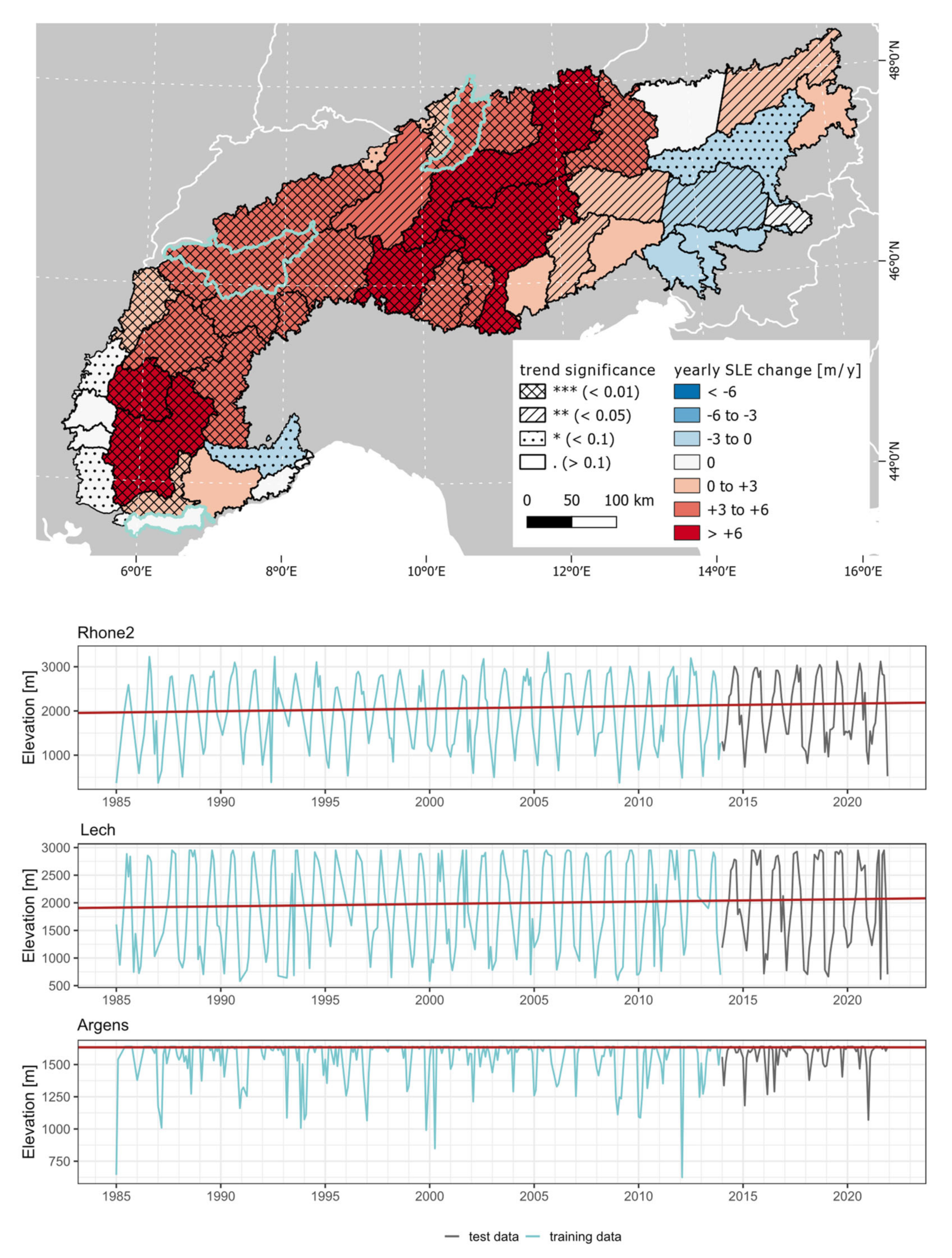
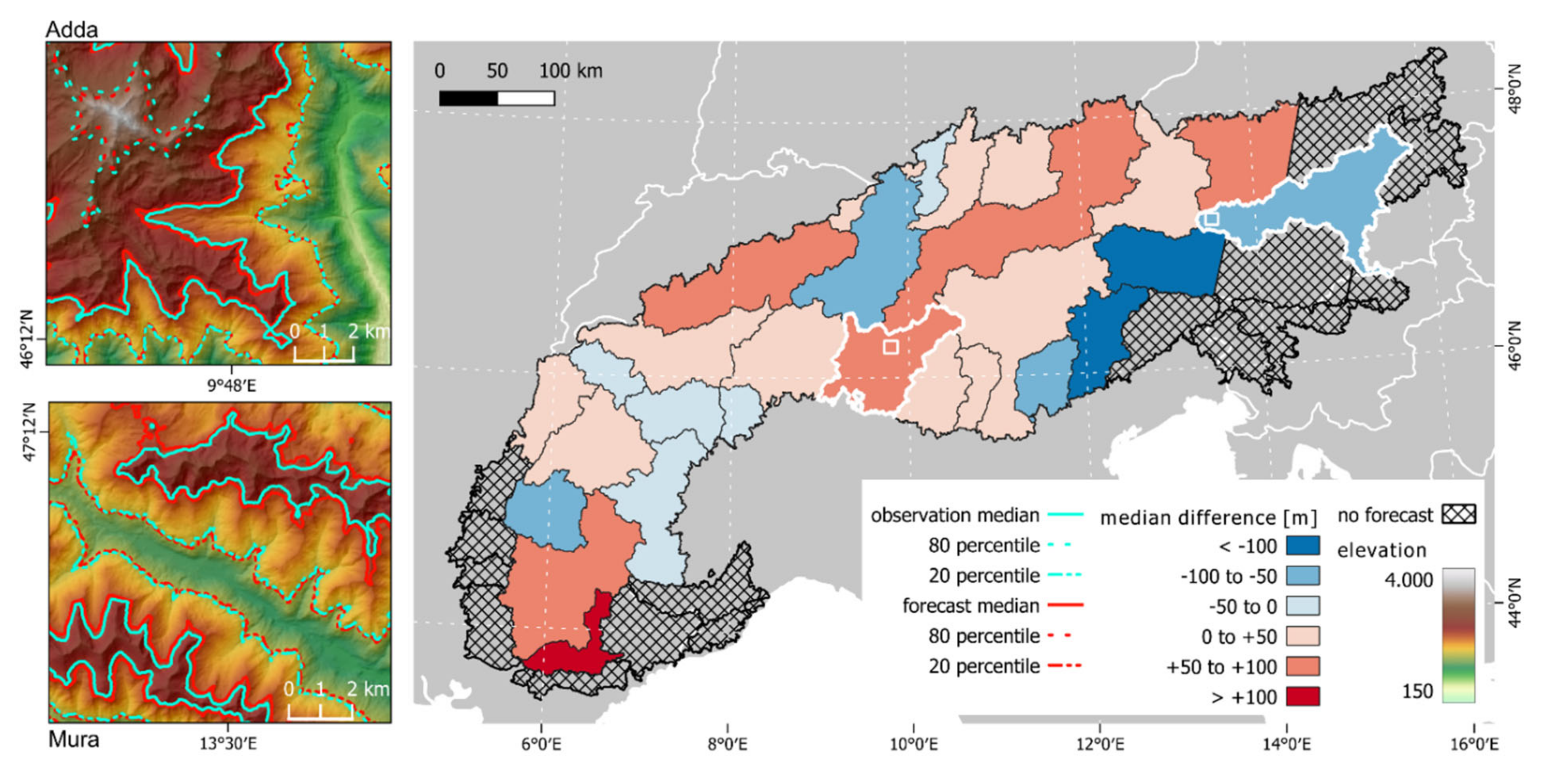
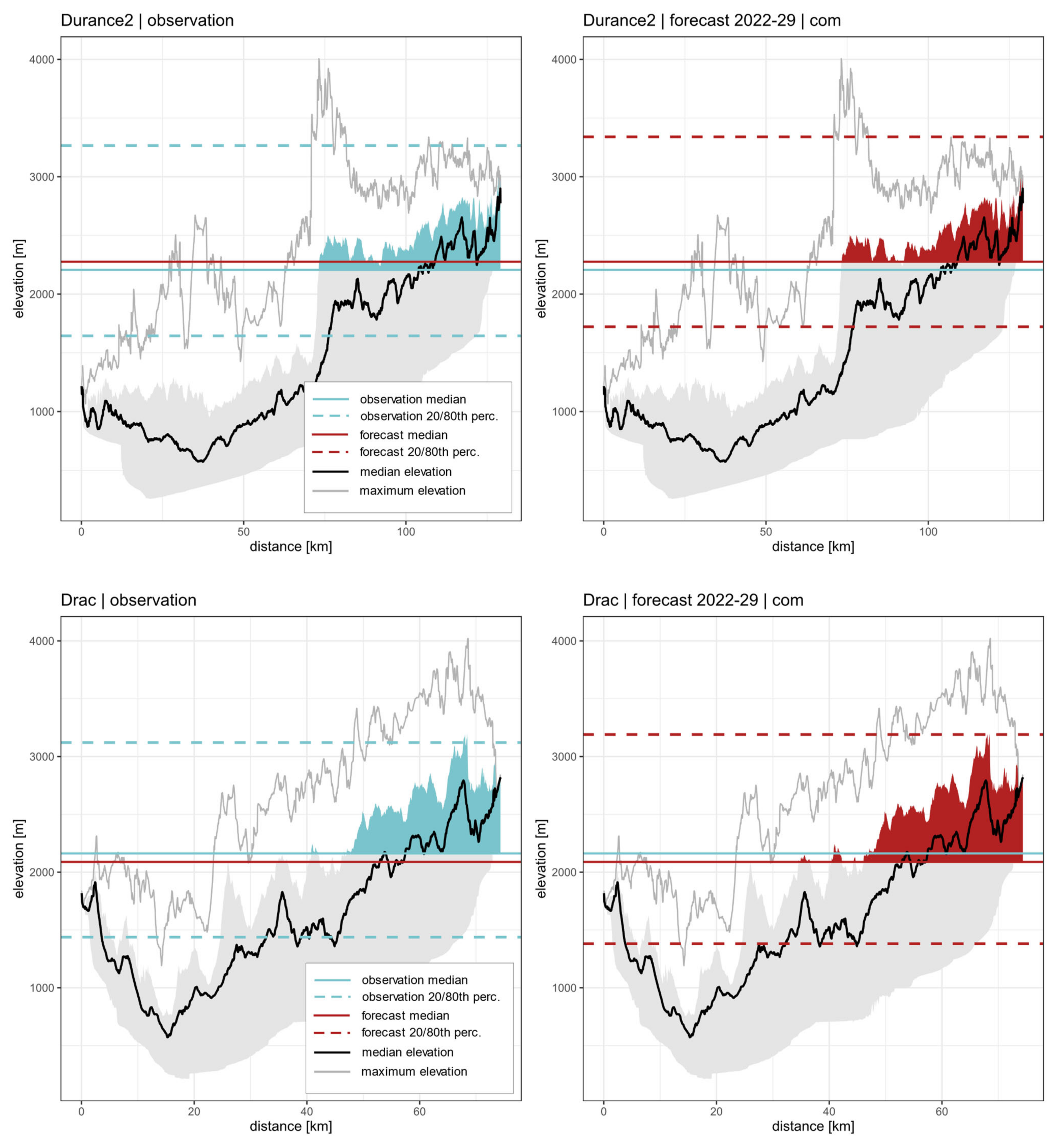
  • We were able to retrieve the SLE from over 14,500 Landsat scenes over 43 Alpine catchments and generated monthly SLE time series ranging from 1985 to 2021. A majority of the Alpine catchments showed a statistically significant positive SLE trend of several meters per year, i.e., the SLE receded to higher elevations in the past 37 years. The strongest SLE trends were observed in the Western Alps in the catchments of Drac (+8.9 m/y) and Upper Durance (+7.3 m/y), while considerably weaker negative trends were also found in the Eastern Alps. The results are well in line with studies that use in situ observations of snow cover. In catchments without any snow in the summer months, no trend was detected.
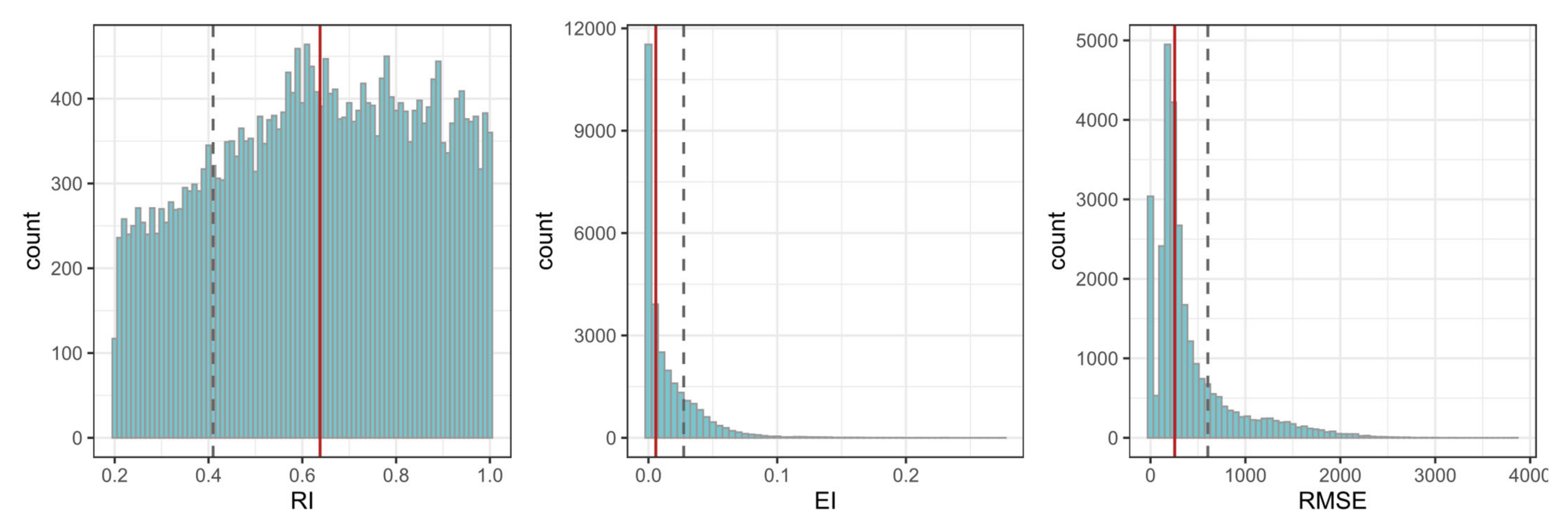
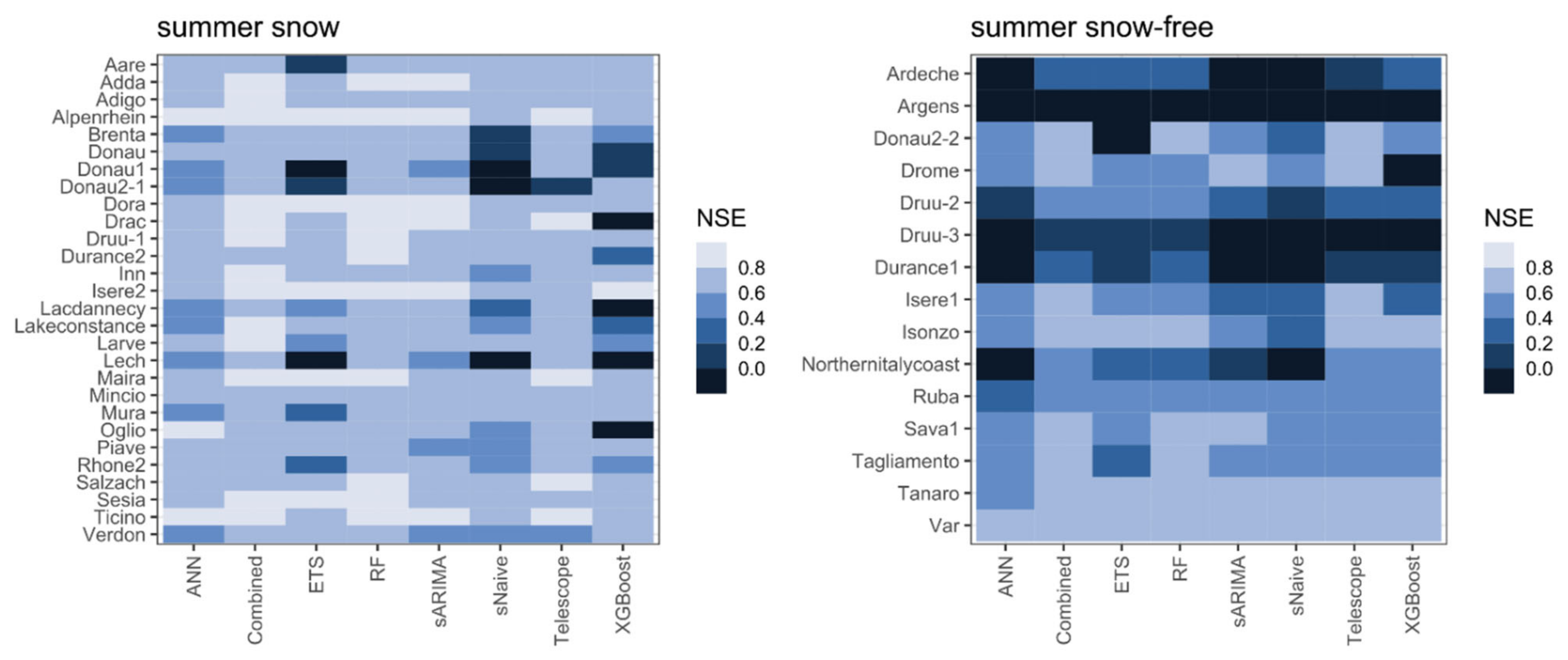
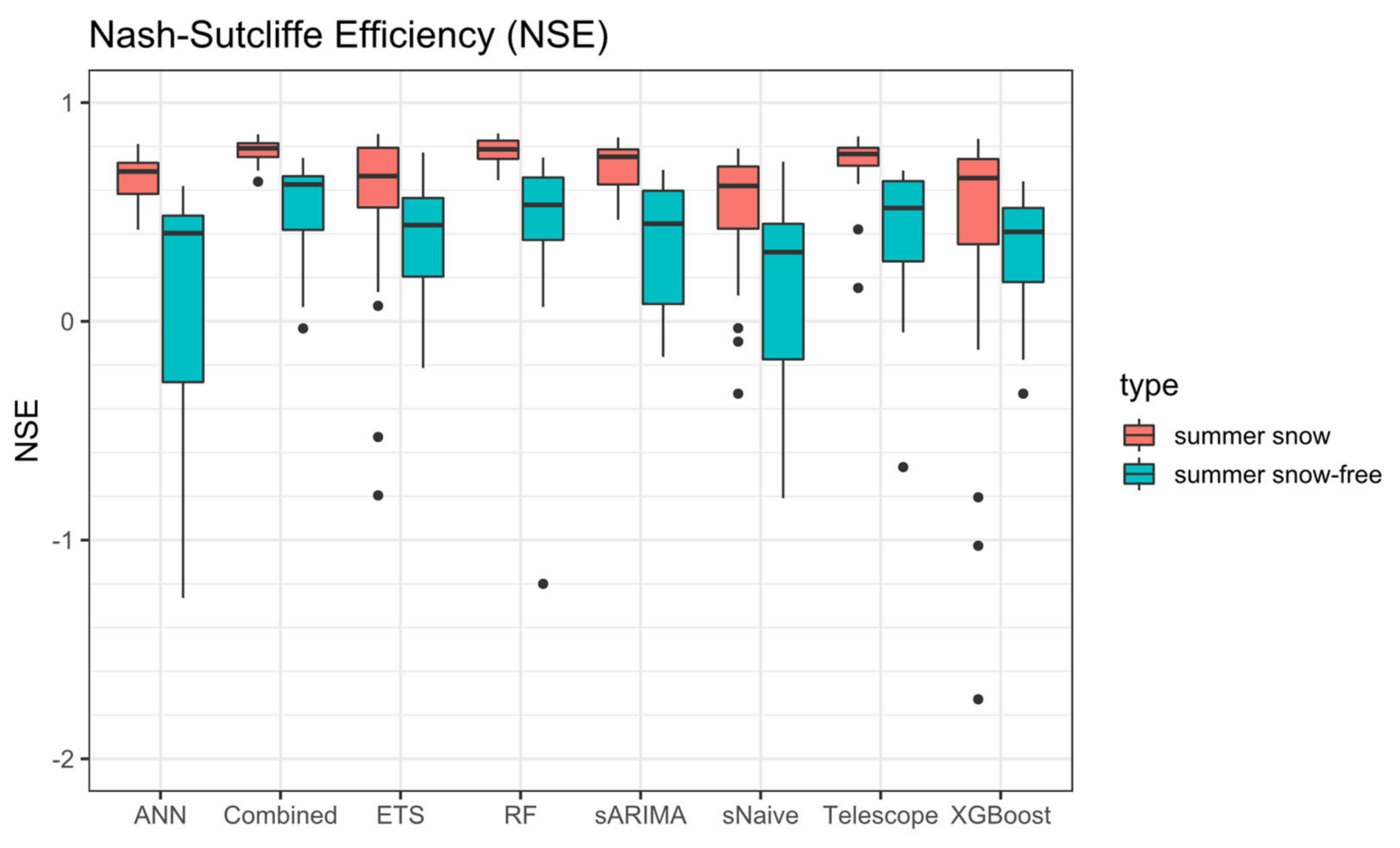
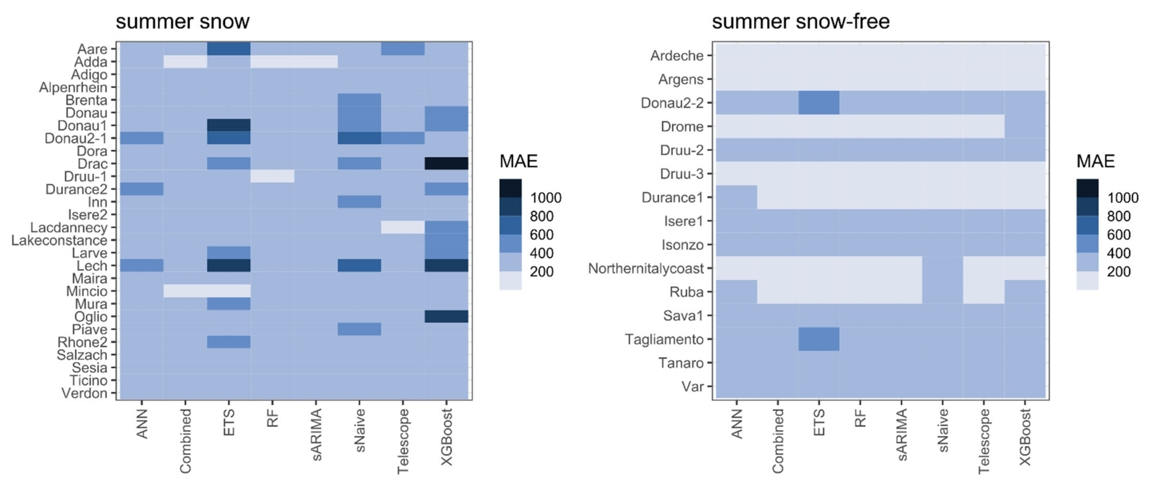
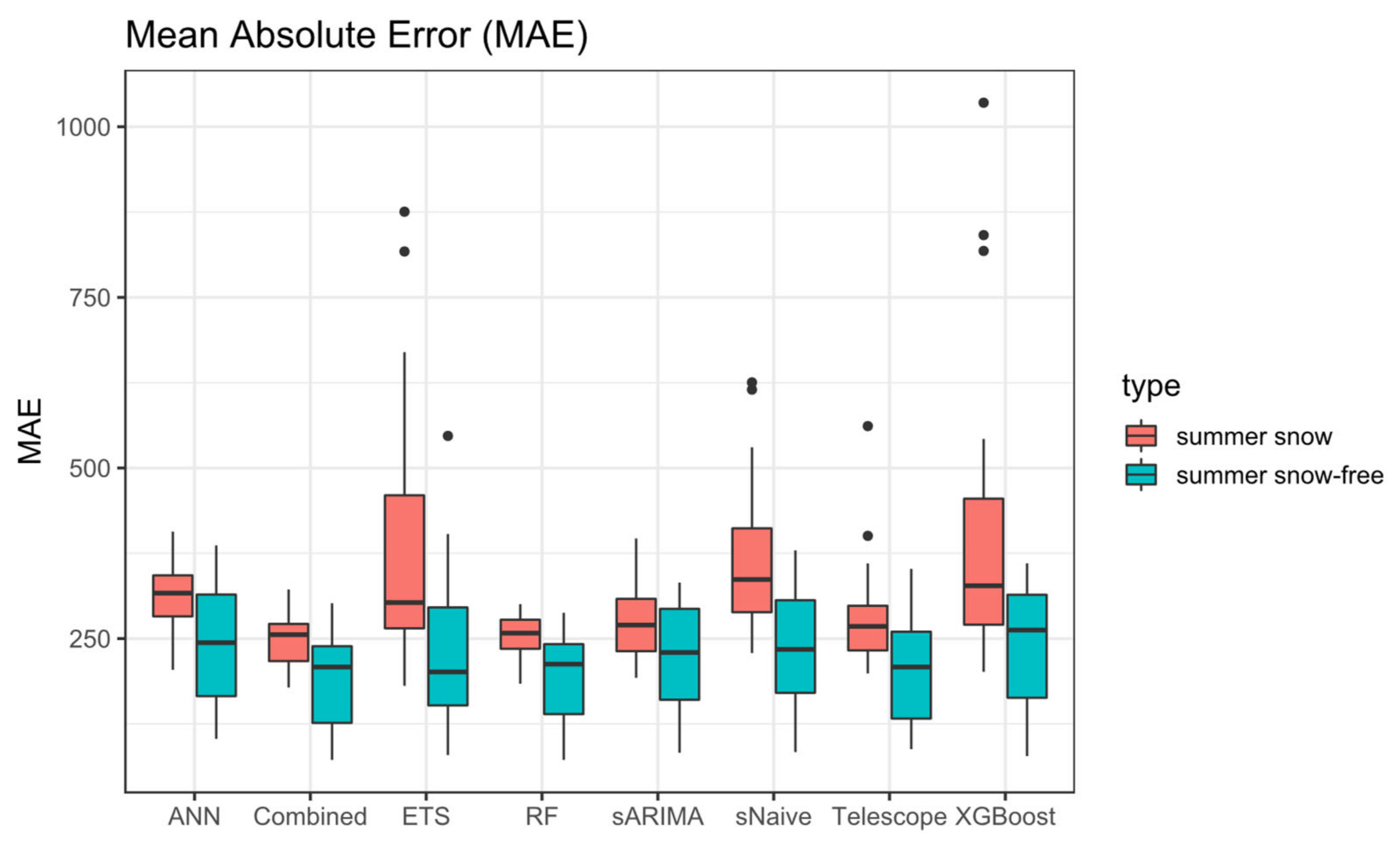
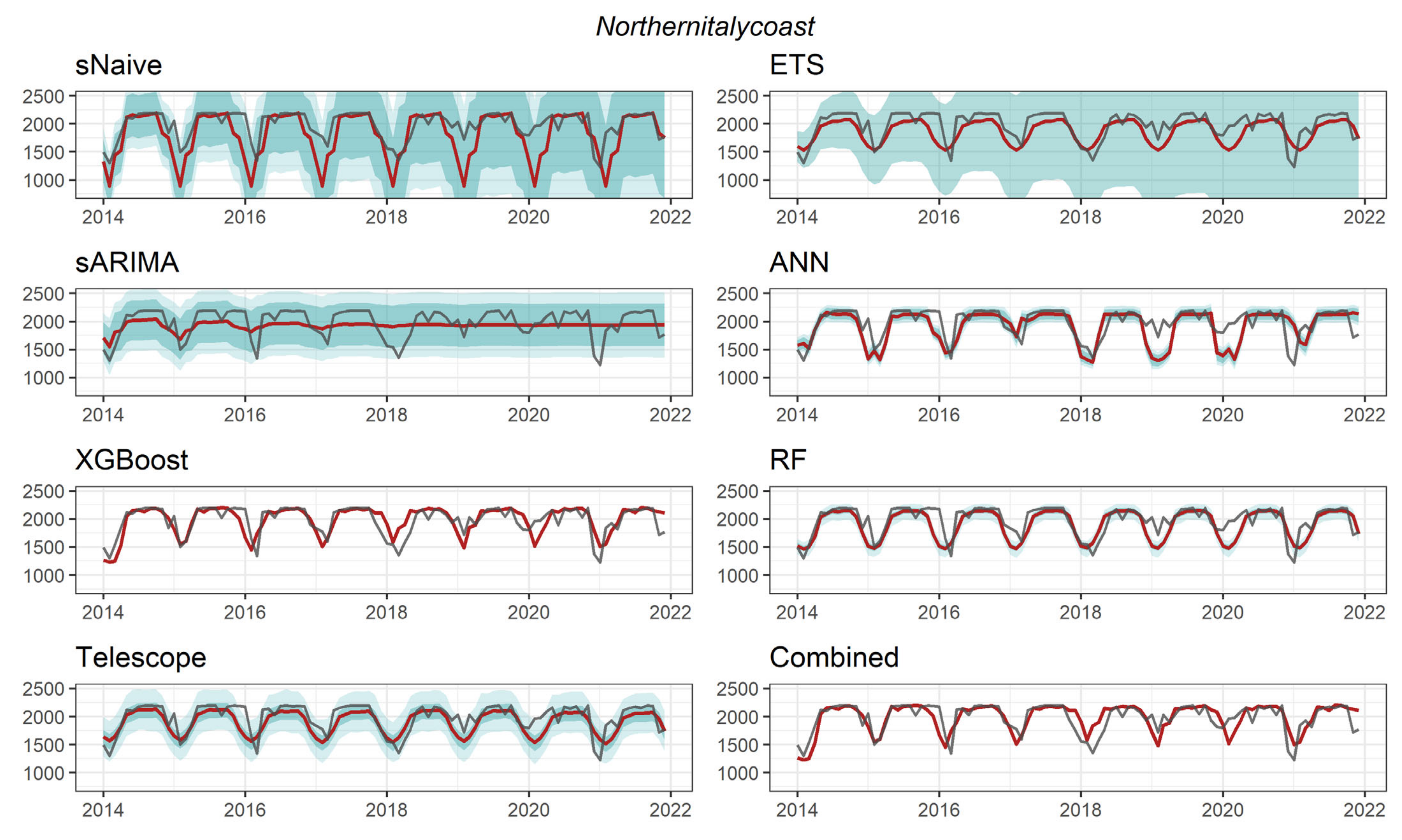
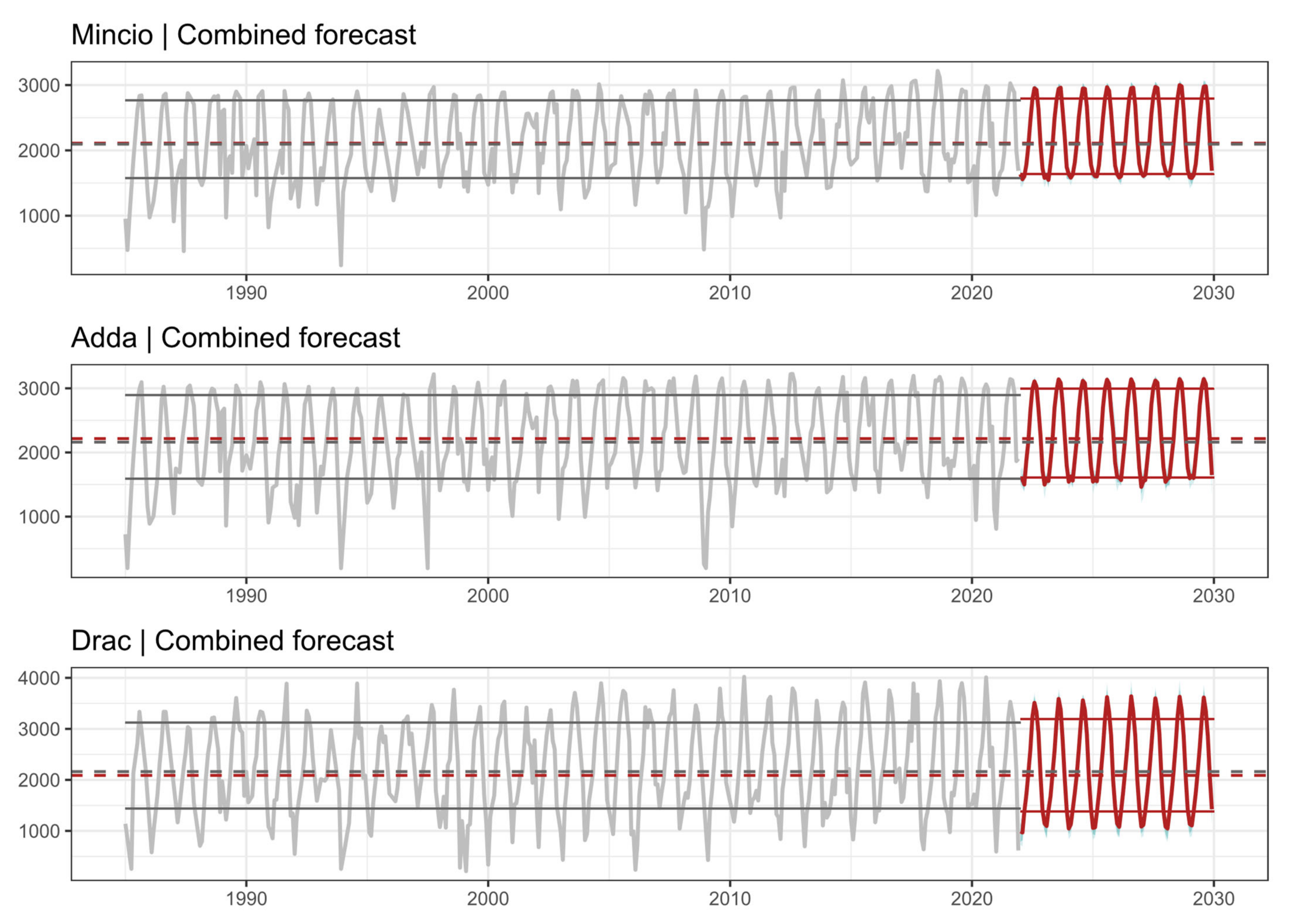
  • The time series were modeled using seven forecasting methods and evaluated on test data that comprise the most recent 20% of the SLE time series. In catchments where snow is present in summer at the highest elevations, the seasonal pattern of the SLE dynamics was captured well by all approaches, with only a few exceptions in single catchments. The best results were achieved by RF (NSE = 0.79, MAE = 258 m), Telescope (0.76, 268 m), and sARIMA (0.75, 270 m). Since the performance of the methods varied between catchments, we introduced a Combined forecast that averaged the best forecasting results by weighting them according to the NSE score. This robust forecast approach achieved an NSE of 0.79 at an MAE of 256 m. In catchments, where the SLE maxes out in summer, the forecast performance was considerably lower and strongly dependent on the input data. Here, the Combined forecast achieved a median NSE of 0.63.
  • Using the Combined forecasting approach, we forecast the SLE time series for 28 of the catchments for the years 2022 to 2029 and compared the SLE distribution to those of the observed time series. In 61% of the catchments, the median SLE difference retained the sign of the calculated long-term trend. A negative SLE shift despite a positive long-term trend was forecast for five catchments in the Eastern Alps, one in the Northern Alps, and three in the Eastern Alps. Possible reasons for that are exemplarily discussed in Drac, considering the properties of the forecasting model, topography, and climate variables.
Based on the findings of this study, we want to highlight the following aspects to further facilitate research on using long EO time series to forecast snow cover dynamics and give an indication towards further research directions:
  • The effort for data preprocessing prior to forecasting to generate a regular time series is a considerable challenge. To further foster EO-based forecasting, we strongly encourage the generation of harmonized analysis-ready data products from long RS time series. Since there are few EO missions that are continuously operational over several decades, a prerequisite for the detection of long-term trends of climate-dependent environmental variables, we advocate that existing missions be continued to ensure an ongoing stream of data. Following the example of the Copernicus program to complement the Landsat time series with the Sentinel-2 mission, the launch of new missions can contribute to the ability to densify time series and facilitate EO-based forecasting.
  • We expect that SLE time series and forecasts can be improved considerably by including physical predictor variables such as climate or meteorological data in a multivariate modeling approach. This would also enable forecasts according to different RCP scenarios and solve the problems of univariate approaches in catchments with maxed-out SLEs. Further consideration will be directed into downscaling the approach to the sub-catchment or administrative boundary level to better meet the needs of local stakeholders and policy and decision makers.
In summary, we demonstrated that it is possible to generate SLE forecasts from long EO-based time series with satisfying accuracy. Future research will especially be directed toward establishing linkages between Alpine-wide SLE dynamics and potential drivers. These efforts will facilitate the implementation of a forecasting framework for snow cover in mountainous regions, which will yield viable information about the future impact of climate change.

Author Contributions

Conceptualization, J.K., A.J.D. and C.K.; Methodology, J.K.; Software, J.K. and A.B.; Supervision, C.K.; Visualization, J.K.; Writing—original draft, J.K.; Writing—review and editing, A.B., A.J.D. and C.K. All authors have read and agreed to the published version of the manuscript.

Funding

This study was supported by the DLR “Polar Monitor” project.

Institutional Review Board Statement

Not applicable.

Informed Consent Statement

Not applicable.

Data Availability Statement

The data presented in this study are available on request from the corresponding author. The data are not publicly available due to their volume.

Acknowledgments

The authors would like to thank Thorsten Hoeser for fruitful discussions about methodology and data visualization, Ka Hei Chow and Ann Christin Kogel for assistance in data processing, and Anna Köhler and David Marshall for final proofreading. The authors are particularly grateful for the valuable suggestions provided by the Academic Editor and three anonymous reviewers, which helped greatly improve this paper.

Conflicts of Interest

The authors declare no conflict of interest.

Appendix A

Table A1. SLE statistics of all Alpine catchments analyzed in this study. The occurrence of summer snow determines whether the SLE maxes out in summer. Trend significance thresholds are determined by the following p-values: *** p < 0.01, ** p < 0.05, * p < 0.1, - p ≥ 0.1. Forecasts for 2022–2029 are only calculated in catchments without a maxed-out SLE, i.e., with presence of summer snow.
IDCatchmentSummer SnowLong-Term Trend [m/y] *Median SLE
1985–2021 [m]
Median SLE
2022–2029 [m]
Median SLE
Difference [m]
1Argensno0 -1634--
2Varno0.43 -2253--
3Northern Italy Coastno0 -2096--
4Tanarono−0.04 *2269--
5Verdonyes2.65 **21162265149
6Durance 1no0 *1834--
7Durance 2yes7.29 ***2206227569
8Mairayes4.03 **22562214−42
9Dracyes8.93 ***21622089−73
10Ardecheno0 -1731--
11Dromeno0 -1841--
12Isere 1no0 *1891--
13Isere 2yes6.00 ***2069209728
14Dorayes5.56 ***21972175−22
15Sesiayes5.22 ***21212108−13
16Lac D’Annecyyes2.46 **1896194347
17L’Arveyes5.62 ***18851873−12
18Rhone 2yes5.74 ***1966200236
19Aareyes4.09 ***1882194765
20Lake Constanceyes1.33 *1644167127
21Alpenrheinyes3.61 **19671898−69
22Donau 1yes2.17 ***17611754−7
23Lechyes4.31 ***191419239
24Donauyes5.18 ***1928196941
25Innyes6.25 ***2000206666
26Salzachyes3.16 ***1882190220
27Donau 2-1yes0 -1918198163
28Donau 2-2no1.99 **1807--
29Ticinoyes5.88 ***2019204021
30Addayes6.65 ***2161221655
31Oglioyes5.50 ***2118215638
32Mincioyes5.66 ***2095211116
33Adigoyes6.92 ***2145218641
34Brentayes1.79 -21582064−94
35Piaveyes2.07 **22132100−113
36Tagliamentono0.20 -2218--
37Druu 1yes2.23 **22482000−248
38Druu 2no−1.09 **2226--
39Druu 3no0 **1532--
40Isonzono−0.40 -1994--
41Savano−0.89 -2083--
42Murayes−2.00 *22022122−80
43Rubano0.34 -1766--
Figure A1. Location of the observed (left, blue) and forecast (right, red) SLE in the topography of the catchments Adda (upper panels) and Mura (lower panels). The topography (black and gray) is depicted as a swath profile from West to East and shows the elevation distribution in North-South transects perpendicular to the swath. The grey area depicts the elevation range in which 80% of the DEM pixels are located. Areas within this 80th elevation percentile that are covered in snow more than 50% of the time (i.e., above the SLE median) are highlighted in color.
Remotesensing 14 04461 g0a1

References

  1. Thackeray, C.W.; Derksen, C.; Fletcher, C.G.; Hall, A. Snow and climate: Feedbacks, drivers, and indices of change. Curr. Clim. Chang. Rep. 2019, 5, 322–333. [Google Scholar] [CrossRef]
  2. Mountain Research Initiative EDW Working Group. Elevation-dependent warming in mountain regions of the world. Nat. Clim. Chang. 2015, 5, 424–430. [Google Scholar] [CrossRef]
  3. Winter, K.J.-P.M.; Kotlarski, S.; Scherrer, S.C.; Schär, C. The alpine snow-albedo feedback in regional climate models. Clim. Dyn. 2017, 48, 1109–1124. [Google Scholar] [CrossRef]
  4. Hock, R.; Rasul, G.; Adler, C.; Cáceres, B.; Gruber, S.; Hirabayashi, Y.; Jackson, M.; Kääb, A.; Kang, S.; Kutuzov, S.; et al. High mountain areas. In IPCC Special Report on the Ocean and Cryosphere in a Changing Climate; Pörtner, H.-O., Roberts, D.C., Masson-Delmotte, V., Zhai, P., Tignor, M., Poloczanska, E., Mintenbeck, K., Alegría, A., Nicolai, M., Okem, A., et al., Eds.; Cambridge University Press: Cambridge, UK; New York, NY, USA, 2019. [Google Scholar]
  5. Rumpf, S.B.; Gravey, M.; Brönnimann, O.; Luoto, M.; Cianfrani, C.; Mariethoz, G.; Guisan, A. From white to green: Snow cover loss and increased vegetation productivity in the European Alps. Science 2022, 376, 1119–1122. [Google Scholar] [CrossRef] [PubMed]
  6. Antão, L.H.; Weigel, B.; Strona, G.; Hällfors, M.; Kaarlejärvi, E.; Dallas, T.; Opedal, Ø.H.; Heliölä, J.; Henttonen, H.; Huitu, O.; et al. Climate change reshuffles northern species within their niches. Nat. Clim. Chang. 2022, 12, 587–592. [Google Scholar] [CrossRef]
  7. Winkler, D.E.; Butz, R.J.; Germino, M.J.; Reinhardt, K.; Kueppers, L.M. Snowmelt timing regulates community composition, phenology, and physiological performance of alpine plants. Front. Plant Sci. 2018, 9, 1140. [Google Scholar] [CrossRef] [PubMed]
  8. Khodaee, M.; Hwang, T.; Ficklin, D.L.; Duncan, J.M. With warming, spring streamflow peaks are more coupled with vegetation green-up than snowmelt in the northeastern United States. Hydrol. Processes 2022, 36, e14621. [Google Scholar] [CrossRef]
  9. Immerzeel, W.W.; Lutz, A.F.; Andrade, M.; Bahl, A.; Biemans, H.; Bolch, T.; Hyde, S.; Brumby, S.; Davies, B.J.; Elmore, A.C.; et al. Importance and vulnerability of the world’s water towers. Nature 2020, 577, 364–369. [Google Scholar] [CrossRef]
  10. Steiger, R.; Scott, D.; Abegg, B.; Pons, M.; Aall, C. A critical review of climate change risk for ski tourism. Curr. Issues Tour. 2019, 22, 1343–1379. [Google Scholar] [CrossRef]
  11. Beniston, M.; Farinotti, D.; Stoffel, M.; Andreassen, L.M.; Coppola, E.; Eckert, N.; Fantini, A.; Giacona, F.; Hauck, C.; Huss, M.; et al. The European mountain cryosphere: A review of its current state, trends, and future challenges. Cryosphere 2018, 12, 759–794. [Google Scholar] [CrossRef] [Green Version]
  12. Hu, Z.; Dietz, A.; Zhao, A.; Uereyen, S.; Zhang, H.; Wang, M.; Mederer, P.; Kuenzer, C. Snow moving to higher elevations: Analyzing three decades of snowline dynamics in the Alps. Geophys. Res. Lett. 2020, 47, e2019GL085742. [Google Scholar] [CrossRef]
  13. Damm, A.; Greuell, W.; Landgren, O.; Prettenthaler, F. Impacts of +2 °C global warming on winter tourism demand in europe. Clim. Serv. 2017, 7, 31–46. [Google Scholar] [CrossRef]
  14. Spandre, P.; François, H.; Verfaillie, D.; Lafaysse, M.; Déqué, M.; Eckert, N.; George, E.; Morin, S. Climate controls on snow reliability in French Alps ski resorts. Sci. Rep. 2019, 9, 8043. [Google Scholar] [CrossRef] [PubMed]
  15. U.S. Geological Survey Landsat—Earth Observation Satellites (Ver. 1.2, April 2020): U.S. Geological Survey Fact Sheet 2015–3081. Available online: https://pubs.er.usgs.gov/publication/fs20153081 (accessed on 13 January 2022).
  16. Koehler, J.; Kuenzer, C. Forecasting spatio-temporal dynamics on the land surface using earth observation data—A review. Remote Sens. 2020, 12, 3513. [Google Scholar] [CrossRef]
  17. Gorelick, N.; Hancher, M.; Dixon, M.; Ilyushchenko, S.; Thau, D.; Moore, R. Google Earth Engine: Planetary-scale geospatial analysis for everyone. Remote Sens. Environ. 2017, 202, 18–27. [Google Scholar] [CrossRef]
  18. Reichstein, M.; Camps-Valls, G.; Stevens, B.; Jung, M.; Denzler, J.; Carvalhais, N.; Prabhat. Deep learning and process understanding for data-driven earth system science. Nature 2019, 566, 195–204. [Google Scholar] [CrossRef] [PubMed]
  19. Dietz, A.J.; Kuenzer, C.; Dech, S. Global SnowPack: A new set of snow cover parameters for studying status and dynamics of the planetary snow cover extent. Remote Sens. Lett. 2015, 6, 844–853. [Google Scholar] [CrossRef]
  20. Hüsler, F.; Jonas, T.; Riffler, M.; Musial, J.P.; Wunderle, S. A satellite-based snow cover climatology (1985–2011) for the European Alps derived from AVHRR data. Cryosphere 2014, 8, 73–90. [Google Scholar] [CrossRef]
  21. Romanov, P. Global multisensor automated satellite-based snow and ice mapping system (GMASI) for cryosphere monitoring. Remote Sens. Environ. 2017, 196, 42–55. [Google Scholar] [CrossRef]
  22. Wu, X.; Naegeli, K.; Premier, V.; Marin, C.; Ma, D.; Wang, J.; Wunderle, S. Evaluation of snow extent time series derived from advanced very high resolution radiometer global area coverage data (1982–2018) in the Hindu Kush Himalayas. Cryosphere 2021, 15, 4261–4279. [Google Scholar] [CrossRef]
  23. Rößler, S.; Dietz, A.J. Detection of snow cover from historical and recent AVHHR data—A thematic TIMELINE Processor. Geomatics 2022, 2, 144–160. [Google Scholar] [CrossRef]
  24. Nagler, T.; Rott, H.; Ripper, E.; Bippus, G.; Hetzenecker, M. Advancements for snowmelt monitoring by means of Sentinel-1 SAR. Remote Sens. 2016, 8, 348. [Google Scholar] [CrossRef]
  25. Tsai, Y.; Dietz, A.J.; Oppelt, N.; Kuenzer, C. Wet and dry snow detection using Sentinel-1 SAR data for mountainous areas with a machine learning technique. Remote Sens. 2019, 11, 895. [Google Scholar] [CrossRef]
  26. Hu, Z.; Dietz, A.J.; Kuenzer, C. Deriving regional snow line dynamics during the ablation seasons 1984–2018 in European mountains. Remote Sens. 2019, 11, 933. [Google Scholar] [CrossRef]
  27. Hu, Z.; Dietz, A.; Kuenzer, C. The potential of retrieving snow line dynamics from landsat during the end of the ablation Seasons between 1982 and 2017 in European mountains. Int. J. Appl. Earth Obs. Geoinf. 2019, 78, 138–148. [Google Scholar] [CrossRef]
  28. Bormann, K.J.; Brown, R.D.; Derksen, C.; Painter, T.H. Estimating snow-cover trends from space. Nat. Clim. Chang. 2018, 8, 924–928. [Google Scholar] [CrossRef]
  29. Marty, C.; Schlögl, S.; Bavay, M.; Lehning, M. How much can we save? Impact of different emission scenarios on future snow cover in the Alps. Cryosphere 2017, 11, 517–529. [Google Scholar] [CrossRef]
  30. Gobiet, A.; Kotlarski, S.; Beniston, M.; Heinrich, G.; Rajczak, J.; Stoffel, M. 21st century climate change in the European Alps—A review. Sci. Total Environ. 2014, 493, 1138–1151. [Google Scholar] [CrossRef] [PubMed]
  31. Alpine Convention Perimeter of the Alpine Convention. 2020. Available online: https://www.atlas.alpconv.org/layers/geonode_data:geonode:Alpine_Convention_Perimeter_2018_v2 (accessed on 13 July 2022).
  32. Wolpert, D.H.; Macready, W.G. No free lunch theorems for optimization. IEEE Trans. Evol. Computat. 1997, 1, 67–82. [Google Scholar] [CrossRef]
  33. Hall, D.K.; Riggs, G.A.; Salomonson, V.V.; DiGirolamo, N.E.; Bayr, K.J. MODIS snow-cover products. Remote Sens. Environ. 2002, 83, 181–194. [Google Scholar] [CrossRef] [Green Version]
  34. Earth Resources Observation and Science (EROS) Center Collection-2 Landsat 8-9 OLI (Operational Land Imager) and TIRS (Thermal Infrared Sensor) Level-2 Science Products. 2013. Available online: https://www.usgs.gov/centers/eros/science/usgs-eros-archive-landsat-archives-landsat-8-9-olitirs-collection-2-level-2 (accessed on 13 July 2022).
  35. Earth Resources Observation and Science (EROS) Center Collection-2 Landsat 7 Enhanced Thematic Mapper Plus (ETM+) Level-2 Science Products. 1999. Available online: https://www.usgs.gov/centers/eros/science/usgs-eros-archive-landsat-archives-landsat-7-etm-plus-collection-2-level-2 (accessed on 13 July 2022).
  36. Earth Resources Observation And Science (EROS) Center Collection-2 Landsat 4-5 Thematic Mapper (TM) Level-2 Science Products. 2020. Available online: https://www.usgs.gov/centers/eros/science/usgs-eros-archive-landsat-archives-landsat-4-5-tm-collection-2-level-2-science (accessed on 13 July 2022).
  37. ESA Copernicus DEM—Global and European Digital Elevation Model (COP-DEM). Available online: https://spacedata.copernicus.eu/web/cscda/dataset-details?articleId=394198 (accessed on 13 July 2022).
  38. Lehner, B.; Grill, G. Global River hydrography and network routing: Baseline data and new approaches to study the world’s large river systems: Global river hydrography and network routing. Hydrol. Process. 2013, 27, 2171–2186. [Google Scholar] [CrossRef]
  39. Ripper, E.; Schwaizer, G.; Nagler, T.; Metsämäki, S.; Törmä, M.; Fernandes, R.; Crawford, C.J.; Painter, T.H.; Rittger, K. Guidelines for the Generation of Snow Extent Products from High Resolution Optical Sensors. 2019. Available online: https://snowpex.enveo.at/doc/D08_Guidelines_for_the_generation_of_snow_extent_products_from_HR_optical_sensors_FINAL_v2.1.pdf (accessed on 13 July 2022).
  40. Klein, A.G.; Hall, D.K.; Riggs, G.A. Improving snow cover mapping in forests through the use of a canopy reflectance model. Hydrol. Processes 1998, 12, 1723–1744. [Google Scholar] [CrossRef]
  41. Poon, S.K.M.; Valeo, C. Investigation of the MODIS snow mapping algorithm during snowmelt in the northern boreal forest of canada. Can. J. Remote Sens. 2006, 32, 254–267. [Google Scholar] [CrossRef]
  42. Metsämäki, S.; Pulliainen, J.; Salminen, M.; Luojus, K.; Wiesmann, A.; Solberg, R.; Böttcher, K.; Hiltunen, M.; Ripper, E. Introduction to GlobSnow Snow Extent products with considerations for accuracy assessment. Remote Sens. Environ. 2015, 156, 96–108. [Google Scholar] [CrossRef]
  43. Hall, D.K.; Riggs, G.A.; Salomonson, V.V. Development of methods for mapping global snow cover using moderate resolution imaging spectroradiometer data. Remote Sens. Environ. 1995, 54, 127–140. [Google Scholar] [CrossRef]
  44. Tucker, C.J. Red and photographic infrared linear combinations for monitoring vegetation. Remote Sens. Environ. 1979, 8, 127–150. [Google Scholar] [CrossRef]
  45. Gao, B. NDWI—A normalized difference water index for remote sensing of vegetation liquid water from space. Remote Sens. Environ. 1996, 58, 257–266. [Google Scholar] [CrossRef]
  46. Zhu, Z.; Wang, S.; Woodcock, C.E. Improvement and expansion of the Fmask algorithm: Cloud, cloud shadow, and snow detection for landsats 4–7, 8, and Sentinel 2 images. Remote Sens. Environ. 2015, 159, 269–277. [Google Scholar] [CrossRef]
  47. Härer, S.; Bernhardt, M.; Siebers, M.; Schulz, K. On the need for a time- and location-dependent estimation of the NDSI threshold value for reducing existing uncertainties in snow cover maps at different scales. Cryosphere 2018, 12, 1629–1642. [Google Scholar] [CrossRef]
  48. Zhao, J.; Shi, Y.; Huang, Y.; Fu, J. Uncertainties of snow cover extraction caused by the nature of topography and underlying surface. J. Arid Land 2015, 7, 285–295. [Google Scholar] [CrossRef]
  49. Burton-Johnson, A.; Black, M.; Fretwell, P.T.; Kaluza-Gilbert, J. An automated methodology for differentiating rock from snow, clouds and seain antarctica from Landsat 8 imagery: A new rock outcrop map and areaestimation for the entire Antarctic continent. Cryosphere 2016, 10, 1665–1677. [Google Scholar] [CrossRef]
  50. Krajčí, P.; Holko, L.; Perdigão, R.A.P.; Parajka, J. Estimation of regional snowline elevation (RSLE) from MODIS images for seasonally snow covered mountain basins. J. Hydrol. 2014, 519, 1769–1778. [Google Scholar] [CrossRef]
  51. Hirsch, R.M.; Slack, J.R.; Smith, R.A. Techniques of trend analysis for monthly water quality data. Water Resour. Res. 1982, 18, 107–121. [Google Scholar] [CrossRef]
  52. Sen, P.K. Estimates of the regression coefficient based on Kendall’s tau. J. Am. Stat. Assoc. 1968, 63, 1379–1389. [Google Scholar] [CrossRef]
  53. Hyndman, R.J.; Athanasopoulos, G. Forecasting: Principles and Practice, 2nd ed.; OTexts: Melbourne, Australia, 2018; ISBN 978-0-9875071-1-2. [Google Scholar]
  54. Hyndman, R.J.; Khandakar, Y. Automatic time series forecasting: The forecast package for R. J. Stat. Soft. 2008, 27, 1–22. [Google Scholar] [CrossRef]
  55. Breiman, L. Random forests. Mach. Learn. 2001, 45, 5–32. [Google Scholar] [CrossRef]
  56. Bauer, A. Automated Hybrid Time Series Forecasting: Design, Benchmarking, and Use Cases. Ph.D. Thesis, Universität Würzburg, Würzburg, Germany, 22 December 2020. [Google Scholar]
  57. Chen, T.; Guestrin, C. XGBoost: A Scalable Tree Boosting System. In Proceedings of the 22nd ACM SIGKDD International Conference on Knowledge Discovery and Data Mining, San Francisco, CA, USA, 13 August 2016. [Google Scholar]
  58. Bauer, A.; Züfle, M.; Grohmann, J.; Schmitt, N.; Herbst, N.; Kounev, S. An Automated Forecasting Framework Based on Method Recommendation for Seasonal Time Series. In Proceedings of the ACM/SPEC International Conference on Performance Engineering, Edmonton, AB, Canada, 20 April 2020. [Google Scholar]
  59. Bauer, A.; Züfle, M.; Herbst, N.; Kounev, S.; Curtef, V. Telescope: An Automatic Feature Extraction and Transformation Approach for Time Series Forecasting on a Level-Playing Field. In Proceedings of the 2020 IEEE 36th International Conference on Data Engineering (ICDE), IEEE, Dallas, TX, USA, 20–24 April 2020. [Google Scholar]
  60. WMO Guidelines on the Calculation of Climate Normals 2017. Available online: https://library.wmo.int/doc_num.php?explnum_id=4166 (accessed on 13 July 2022).
  61. Gupta, H.V.; Kling, H.; Yilmaz, K.K.; Martinez, G.F. Decomposition of the mean squared error and NSE performance criteria: Implications for improving hydrological modelling. J. Hydrol. 2009, 377, 80–91. [Google Scholar] [CrossRef]
  62. Nash, J.E.; Sutcliffe, J.V. River flow forecasting through conceptual models part I—A discussion of principles. J. Hydrol. 1970, 10, 282–290. [Google Scholar] [CrossRef]
  63. Knoben, W.J.M.; Freer, J.E.; Woods, R.A. Technical note: Inherent benchmark or not? Comparing nash–sutcliffe and kling–gupta efficiency scores. Hydrol. Earth Syst. Sci. 2019, 23, 4323–4331. [Google Scholar] [CrossRef]
  64. Hyndman, R.J.; Koehler, A.B. Another look at measures of forecast accuracy. Int. J. Forecast. 2006, 22, 679–688. [Google Scholar] [CrossRef] [Green Version]
  65. Matiu, M.; Crespi, A.; Bertoldi, G.; Carmagnola, C.M.; Marty, C.; Morin, S.; Schöner, W.; Cat Berro, D.; Chiogna, G.; De Gregorio, L.; et al. Observed snow depth trends in the European Alps: 1971 to 2019. Cryosphere 2021, 15, 1343–1382. [Google Scholar] [CrossRef]
  66. Vernay, M.; Lafaysse, M.; Monteiro, D.; Hagenmuller, P.; Nheili, R.; Samacoïts, R.; Verfaillie, D.; Morin, S. The S2M meteorological and snow cover reanalysis over the French Mountainous Areas: Description and evaluation (1958–2021). Earth Syst. Sci. Data 2022, 14, 1707–1733. [Google Scholar] [CrossRef]
  67. Beaumet, J.; Ménégoz, M.; Morin, S.; Gallée, H.; Fettweis, X.; Six, D.; Vincent, C.; Wilhelm, B.; Anquetin, S. Twentieth century temperature and snow cover changes in the French Alps. Reg. Environ. Chang. 2021, 21, 114. [Google Scholar] [CrossRef]
Figure 1. Environmental, societal, and economic effects of snow line elevation (SLE) dynamics in mountainous regions. Multi-decadal time series of SLE dynamics observed from remote sensing satellites can be used to forecast future SLE. The forecasts can be used by stakeholders and policy and decision makers to adapt to future SLE dynamics caused by climate change. Several graphics were modified courtesy of the Integration and Application Network, University of Maryland Center for Environmental Science, https://ian.umces.edu/media-library/symbols/ (access on 18 July 2022).
Remotesensing 14 04461 g001
Figure 2. Topography and location of the hydrological catchments in the European Alps. Alpine region delimited by the Alpine convention [31], catchment boundaries according to the HydroSHEDS dataset. Background shows the Copernicus DEM.
Remotesensing 14 04461 g002
Figure 3. Workflow of the steps of analysis performed in this study. In the first step, SLE time series are retrieved using EO data and a DEM (yellow box). In the second step, the raw time series are then filtered for quality and processed to yield regular monthly time series. With these time series, forecast models are trained and evaluated (blue box). Using a combination of the best performing forecasts (purple box), an actual SLE forecast up to the year 2029 is generated (red box).
Remotesensing 14 04461 g003
Figure 4. Example for the processing steps performed during the SLE retrieval. Left: Landsat 8 surface reflectance RGB false color image of a part of the Upper Rhone catchment. The river Rhone is visible in the center of the image. Center: Snow classification derived from the same scene. Transparent areas, where the RGB image is visible are classified as “clear land”. Right: SLE for the entire catchment derived from the snow classification. On 4 March 2020, the SLE at the Upper Rhone catchment is located at 1105 m.a.s.l.
Remotesensing 14 04461 g004
Figure 5. Representative Index (RI), Error Index (EI), and Root Mean Square Error (RMSE) of all derived SLE observations. The red vertical line marks the median value, the dashed line the 20th (RI) and 80th (EI, RMSE) percentiles, respectively. RImedian = 0.64, RI20th = 0.41, EImedian = 0.006, EI80th = 0.027, RMSEmedian = 255, RMSE80th = 605.
Remotesensing 14 04461 g005
Figure 6. Map showing the calculated long-term SLE change trends [m/y] for all analyzed Alpine catchments (above). Three examples of monthly SLE time series from 1985 from the catchments of the rivers Rhone, Lech, and Argens (below). The red line shows the long-term linear trend calculated over the entire time series. The sample catchments are highlighted in the map.
Remotesensing 14 04461 g006
Figure 7. Nash–Sutcliffe efficiency (NSE) of the evaluated forecasting approaches in catchments where the SLE is not maxed out (left) and where it is maxed out (right) in the summer months. Lighter colors indicate better performance. An NSE of 1 is a perfect forecast, while an NSE < 0 indicates that the mean of all observations would yield a better forecast than the model.
Remotesensing 14 04461 g007
Figure 8. Nash–Sutcliffe efficiency (NSE) of the evaluated forecasting approaches across all catchments. A major negative outlier of XGBoost in one summer snow-free catchment (NSE ≈ −4) is not displayed. An NSE of 1 is a perfect forecast, while an NSE < 0 indicates that the mean of all observations would yield a better forecast than the model.
Remotesensing 14 04461 g008
Figure 9. Mean Absolute Error (MAE) of the evaluated forecasting approaches in catchments where the SLE is not maxed out (left) and where it is maxed out (right) in the summer months. Lighter colors indicate better performance. The MAE can be interpreted as the mean absolute deviation of the predicted data from the observations in meters.
Remotesensing 14 04461 g009
Figure 10. Mean Absolute Error (MAE) of the evaluated forecasting approaches across all catchments. The MAE can be interpreted as the mean absolute deviation of the predicted data from the observations in meters.
Remotesensing 14 04461 g010
Figure 11. Qualitative comparison of observed (gray) and forecast (red) SLE of the Drac catchment for the time interval 2014–2021. Where applicable, the 80% and 95% confidence interval (blue shades) is provided. The Combined forecast is calculated from ETS, sARIMA, ANN, RF, and Telescope. The weak performance of XGBoost may be a result of the high variance in the input SLE time series.
Remotesensing 14 04461 g011
Figure 12. Qualitative comparison of observed (gray) and forecast (red) SLE of the Northern Italy Coast catchment for the time interval 2014–2021. Here, the SLE maxes out in the summer months and stays at the highest possible elevation in the catchment for multiple consecutive months. Where applicable, the 80% and 95% confidence interval (blue shades) is provided. Since no method exceeds the NSE threshold of 0.6, only the best performing forecasting method is used for the Combined forecast, which is XGBoost (NSE = 0.47).
Remotesensing 14 04461 g012
Figure 13. Observed (grey) and forecast (red) SLE time series for the catchments Mincio, Adda, and Drac. Dashed lines show the median values of the observed (grey) and forecast (red) time series; thin solid lines show the 20th and 80th percentile. While the median SLE is projected to increase in the coming years in Mincio (+16 m) and Adda (+55 m), a negative change is modeled for Drac (−74 m). See further discussion in Section 4.3. The forecasts were generated using the Combined forecasting scheme.
Remotesensing 14 04461 g013
Figure 14. Difference between the medians of the observed time series (1985–2021) and the forecast time series (2002–2029) for each Alpine catchment (map on the right). Positive values indicate that the median SLE in the future is higher than in the observed past. Forecasts are only conducted in catchments without a maxed-out summer SLE. The forecasts were generated using the Combined forecast approach. The panels on the left show two examples of the observed (blue) and forecast (red) SLE in the catchments Adda and Mura. Solid lines indicate the location of the median and the dashed lines indicate the 20th and 80th percentile, which correspond to the winter and summer SLE, respectively. Note that the detail of Mura does not show the 80th percentile since it only covers very small parts of the catchment located outside of the map extent. Catchments and extents of the details are highlighted on the map.
Remotesensing 14 04461 g014
Figure 15. Location of the observed (left, blue) and forecast (right, red) SLE in the topography of the catchments Upper Durance (upper panels) and Drac (lower panels). The topography (black and gray) is depicted as a swath profile from west to east and shows the elevation distribution in north–south transects perpendicular to the swath. The grey area depicts the elevation range in which 80% of the DEM pixels are located. Areas within this 80th elevation percentile that are covered in snow more than 50% of the time (i.e., above the SLE median) are highlighted in color.
Remotesensing 14 04461 g015
Publisher’s Note: MDPI stays neutral with regard to jurisdictional claims in published maps and institutional affiliations.

