Monitoring of Plastic Islands in River Environment Using Sentinel-1 SAR Data

Abstract

Plastics in the river environment are of major concern due to their potential pathways into the ocean, their persistence in the environment, and their impacts on human and marine health. It has been documented that plastic concentrations in riparian environments are higher following major rain events, where plastic can be moved through surface runoff. Considering the hazard that plastic waste poses to the environment, monitoring techniques are needed to aid in locating, monitoring, and remediating plastic waste within these systems. Dams are known to trap sediments and pollutants, such as metals and Polychlorinated Biphenyls (PCBs). While there is an established background on the monitoring of dams using the synoptic coverage provided by satellite imaging to observe water quality and volume, the detection of marine debris in riparian systems remains challenging, especially in cloudy conditions. Herein, we exploit the use of Synthetic Aperture Radar (SAR) to understand its capabilities for monitoring marine debris. This research focuses on detecting plastic islands within the Drina River system in Bosnia and Herzegovina and Serbia. Here, the results show that the monitoring of these plastic accumulations is feasible using Sentinel-1 SAR data. A quantitative analysis of detection performance is presented using traditional and state-of-the-art change detectors. The analysis of these detectors indicates that detectors that can utilise the coherent data from Single Look Complex (SLC) acquisitions are perform better when compared with those that only utilise incoherent data from Ground Range-Detected (GRD) acquisitions, with true positive detection ratings of ~95% with 0.1% false alarm rates seen in the best-performing detector. We also found that that the cross-pol VH channel provides better detection than those based on single-pol VV polarisation.

1. Introduction

Marine plastic pollution is of major concern due to its persistence in the marine environment and its impacts on human and marine health. The presence of plastic in marine environments has been shown to negatively affect at least 690 species worldwide [1], and this can be through entanglement and/or ingestion [2]. The implications of the human consumption of marine plastic debris are poorly studied; however, concerns have been raised regarding chemical toxicity and the threats posed by the particles themselves inside the body [3,4,5].

A large amount of marine plastic pollution can be derived from land-based sources, such as street litter, poorly controlled waste sites, plastic packaging (industrial or commercial), and illegal dumping [6]. Jambeck et al. (2015) [7] estimate that of the 275 million metric tons of plastic waste generated in 192 coastal countries, 4.8–12.7 million metric tons entered the ocean in 2010. It was also predicted that cumulative quantities of plastic entering the oceans from land-based sources would increase by an order of magnitude by 2025. Following this, Borelle et al. (2020) [8] estimated that 19–23 million metric tons of plastic waste entered aquatic ecosystems in 2016 and predicted that by 2030 annual emissions of plastic waste may increase to 53 million metric tons per years.

Plastics in the river environment are of particular interest due to their potential pathways into the ocean. Lebreton et al. (2017) [9] estimate that between 1.15 and 2.41 million metric tons of plastic waste enters the ocean every year from rivers, with over 74% of emissions occurring between May and October. Previous studies have shown that the observed plastic concentrations within sampled river systems can differ by several orders of magnitude [10]. This change in plastic concentration can be influenced by the population density within the catchment [11]; the presence of dams, weirs, or other artificial barriers [12]; and rainfall rates, where plastic can be moved through surface runoff [13]. Moore et al. (2011) [14] studied the Coyote Creek tributary, the Los Angeles River, and the San Gabriel River, where they reported that plastic debris levels varied by up to three orders of magnitude when measured at different time periods. The significant changes in the plastic concentrations were explained by rainfall events throughout the study, where runoff transported plastic into the riverine system.

Plastics in water are traditionally measured using in situ methods, such as marine trawls [15], biological sampling [16], sediment sampling [17], marine observational surveys [18], and beach combing [19]. More recently, research into the use of remote sensing for plastic monitoring has been implemented. This has primarily been focussed on the use of optical data [20,21], but challenges can arise from cloud cover and resolution issues; thus, other methods to detect plastic debris from remote sensors have started to be explored.

Biermann et al. (2020) [20] used optical satellite data from Sentinel-2 to classify floating debris material consisting of seaweed, sea foam, and macroplastics. Using a Naïve Bayes algorithm to classify mixed materials, the materials were classified as plastics with an accuracy of 86%. Garcia-Garin (2021) [22] used 3700 optical images from drones and aircrafts to train a convolutional neural network (CNN) for detecting floating marine litter. The highest model accuracy achieved was 0.81 during the cross-validation, but the authors suggested that the monitoring of marine litter in the open sea still proposes a technological challenge.

Gomez et al. (2022) [23] found that debris was visible in the River Drina near Visegrad in Sentinel-2 imagery. Using a learning-based approach, the authors found that debris accumulation within the River Drina at Visegrad was highest at the beginning of the year and quickly decreases as the net that intercepts floating garbage within the river is cleared. Their approach could correctly identify floating debris in images that were not from regions used in the training datasets. The authors report that the difficulty of using Sentinel-2 is related to the coarse resolution and its unavailability during cloud cover. This makes analysis after storms and during winter or rainy seasons difficult or impossible.

Synthetic Aperture Radar (SAR) is an active microwave fine-spatial resolution imaging sensor that can monitor in all light conditions and in almost all-weather conditions [24]. SAR is sensitive to surface roughness [25,26], making it particularly valuable in monitoring rivers, oceans, and other surface waters [25,26,27,28,29]. Inland water bodies within SAR images tend to appear relatively smooth, with the energy from the radar reflecting in a specular direction away from the sensor and a small backscatter returning towards the radar [30]. However, water bodies can also have an increased surface roughness created by water currents or wind-stress. This increased surface roughness provokes a higher backscattering, known as Bragg scattering [31].

Dams are known to trap sediments as well as pollutants, such as plastics, metals, and Polychlorinated Biphenyls (PCBs) [32,33]. Optical data and SAR have both been utilised in the monitoring of chlorophyll-a, Total Suspended Matter (TSM), landslide monitoring, and water volumes in dam and reservoir contexts [34,35]. Molkov et al. (2019) [34] used LiDAR and Sentinel-2 data to develop regional algorithms of chlorophyll-a and TSM from the Gorky Reservoir, Russia. The proposed algorithms were capable of being used for the regular environmental monitoring of the Gorky reservoir, and could potentially be adapted for seven other reservoirs in the Volga River system. Reyes-Carmona et al. (2020) [35] used Differential Interferometric Synthetic Aperture Radar (DInSAR) to study the Rules dam, Spain, where ground instabilities for landslides and water level were monitored. Using DInSAR, the group could evaluate potential hazards related to different landslide typologies and could also observe how water level changes within the reservoir influence landslide behaviour [35]. Recently, reports of plastic islands accumulating by dams following heavy rainfall have been reported in Balkan countries [36]. This study is focused on the ability to detect and monitor these accumulated plastic islands using dual-polarimetric SAR.

Direct measurements of marine debris from satellite platforms are deemed critical for the comprehensive monitoring of the issue [37]. Recently, the use of SAR for detecting marine plastics has started being investigated [38,39]. However, particularities in the composition and size of marine debris and their interactions with the ocean background can make the direct detection of plastics using SAR data very challenging [38]. A lack of test cases of SAR imagery for detecting marine debris of various forms (plastic and non-plastic) means that the capabilities of the platform are still largely unknown [40].

In this study, we test—for the first time—the use of coherence detectors with Single Look Complex (SLC) SAR data for the detection of plastic. We present the accuracies and false alarm rates for our new method. We produce heatmaps of multiple sections of the chosen river system in Serbia and Bosnia & Herzegovina showing the plastic accumulation presence/coverage over a 2-year timeframe, and we discuss how these can be used to support management practices within the area.

2. Materials and Methods

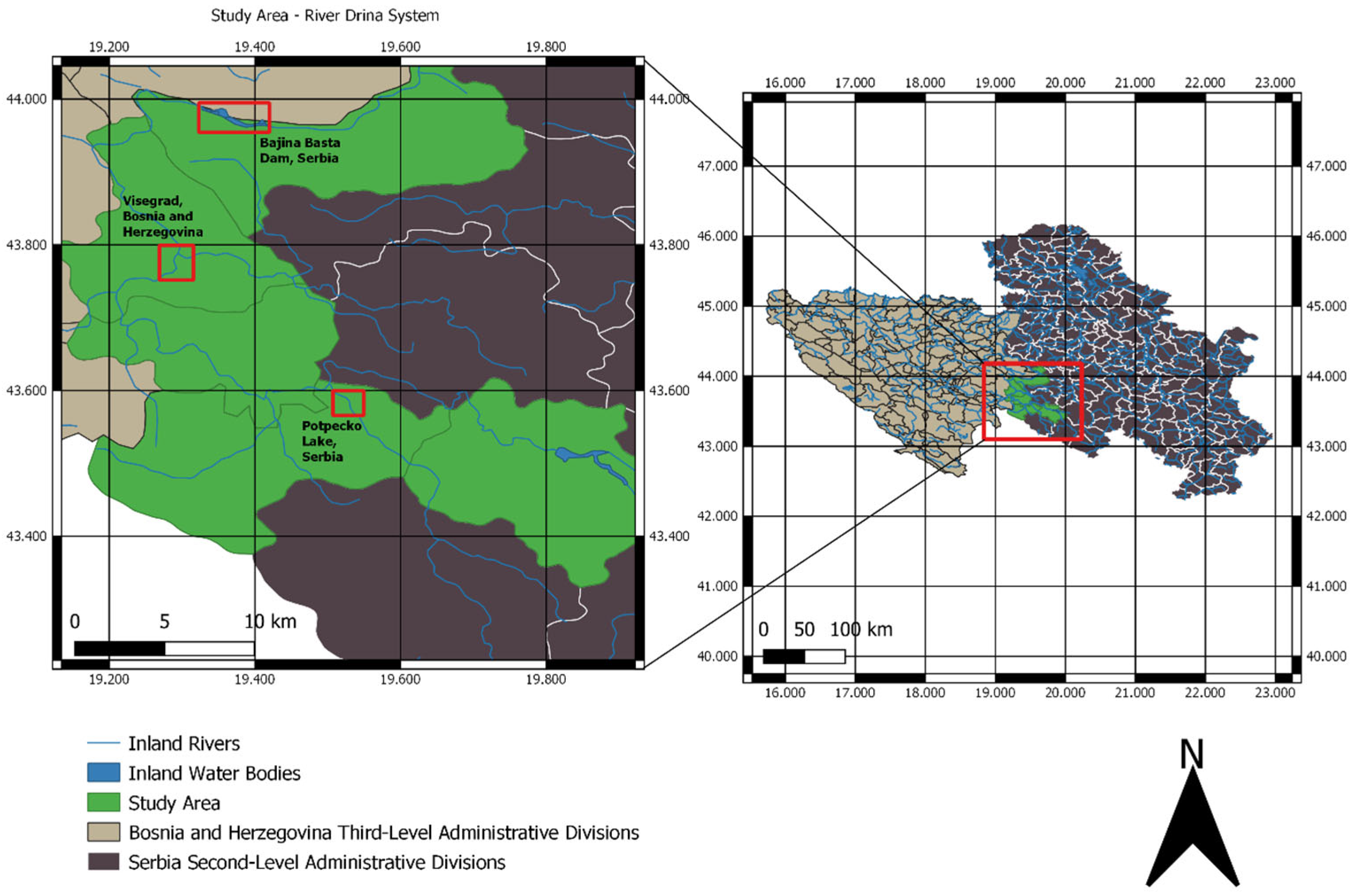
2.1. Study Area

The Balkans constitutes a geographic area in south-eastern Europe, usually characterised as comprising Albania, Bosnia and Herzegovina, Bulgaria, Croatia, Kosovo, Montenegro, North Macedonia, Romania, Serbia, and Slovenia. Waste management assessment of Balkan countries has found key issues within the regions [41]. Regions of Balkans, specifically Bosnia and Herzegovina and Serbia, experienced heavy rainfall in early January 2021 and consequently plastic waste and debris was washed into the river systems.

This study focuses on Potpecko Lake, Serbia and the River Drina, Bosnia and Herzegovina. These regions were selected for monitoring after reports of plastic accumulation near prominent dams in these locations on 5 and 6 January 2021. Pictures taken of the dam during this event provided validation data. A third location, Bajina Basta hydroelectric dam, in Perućac, Serbia, was also located as it is part of the same Drina River system. While there were no reports of plastic accumulations at this third location, we undertook some analyses to understand the river system more comprehensively and to cross-check an area that was reported as clear. A map highlighting the study area and inland hydrology is shown below in Figure 1.

2.2. Satellite Data

In this study, we used dual-polarimetric Sentinel-1 SAR data (5.405 GHz), provided by the European Space Agency (ESA) through the Copernicus Programme (https://scihub.copernicus.eu/dhus/#/home) (accessed on 5 January 2022). The mode of acquisition was Interferometric Wide Swath (IW) SLC. The spatial resolution of the SAR images was approximately 20 × 5 m with a temporal resolution of up to 6 days (12 days using a single orbit). A total of 142 SLC images were downloaded from 5 January 2019 to 26 December 2021, which were used for single image analysis and change detection analysis.

High resolution optical images from Sentinel-2 were acquired; however, cloud cover was 90+% in all images near the date of plastic build-up, so they were inadequate for use for comparison.

2.3. SAR Pre-Processing

In this research, we used Ground Range-Detected (GRD) products to quickly identify locations with marine debris accumulation near the dams. GRD products are SAR data that are calibrated (sigma naught), multi-looked, and projected to ground range using an Earth ellipsoid model; this results in the SAR product having reduced speckle. However, beside these preliminary analyses in this research, we wanted to gain a deeper understanding of the best detection methodologies to evaluate plastic accumulations. Therefore, we also used SLC products to consider information on both amplitude and phase of the received electromagnetic wave. Therefore, we could capitalise on polarimetric information, where we evaluated elements of the polarimetric covariance matrix that consisted of co-polarisation intensity (VV), cross-polarisation intensity (VH), and their cross-correlation (VV * VH), where V stands for vertical linear and H stands for horizontal linear. Sentinel-1 SLC images were processed in the Sentinel Application Platform (SNAP). These images were calibrated and debursted; then, subsets were created of the regions and polarimetric matrices were established with a 1 × 4 multilook to reduce noise before undergoing ellipsoid correction.

To undertake temporal analysis on SAR imaging, pixel-to-pixel matching between features is required within stacked SAR images. Co-registration can align SAR images within a fraction of a pixel [44] and was therefore used to process the datasets of each region in such a way that the same pixels correspond to the same location over the entire temporal stack [45].

2.4. Image Analysis

The dual-polarimetric Sentinel-1 GRD measurements were processed using SNAP. Inspecting the GRD images of Potpecko Lake and River Drina over multiple dates of acquisition showed that there was a clear backscatter difference near the dams before and after 5 January 2021, the date of plastic accumulation, as discussed in Section 3.

Photographs from news reports were used to identify regions of interest (ROIs) where plastic accumulation was present. The ROIs were created as shapefiles (polygons) of Clean (No Plastic) and Accumulated (Plastic Accumulation) regions.

Analysis of the images was then undertaken for the dates where ground evidence was available. The VV, VH intensity, and the Ratio of all pixels were extracted from within the ROI to provide quantitative comparisons. Histograms were then created using the values from the Clean and Accumulated pixel values from within the polygons, further illustrating the differences in backscatter values between the dates of acquisition.

2.5. Classifying Plastic Accumulation

We set the detection task of separating a pixel into two classes. The first class was denoted ‘clean’, which represents pixels of water within the river systems that do not have plastic accumulations. These masks were taken from days where no plastic accumulations were reported in the rivers. The second class is defined as ‘accumulated’; this includes the presence of plastic accumulations

2.6. Change Detection Methods

The change detectors were used to compare references images with the rest of the stack. These images were selected from dates where no plastic accumulation was reported within the river systems (we also visually inspected them to ensure that no debris was present).

Traditional incoherent (not using the phase) detectors were used on each of the test images, including Difference, Normalised Difference, and Ratio Detectors in VV and VH polarisation channels. Newer coherent detectors (using the phase information) were also used and compared to the benchmark traditional detectors, including Optimisation of Power Difference, Optimisation of Power Ratio [46,47,48], and the Hotelling–Lawley trace [49] detectors.

In the following, the main equations and references are provided for each detector.

Difference: This detector considers a reference image, and it subtracts this by the stack of images (pixel by pixel). It is referred to as Diff_XX, where XX represents the polarisation channel (e.g., Diff_VH).

The equation is:

$$\mathsf{\Delta }I=|\langle |im{g}_1{|}^2\rangle -\langle |im{g}_2{|}^2\rangle |>T_1$$

(1)

Normalised Difference is referred to as NDiff_XX:

The equation is:

$$\mathsf{\Delta }{I}_n=\frac{|\langle |im{g}_1{|}^2\rangle -\langle |im{g}_2{|}^2\rangle |}{\langle |im{g}_1{|}^2\rangle +\langle |im{g}_2{|}^2\rangle }>T_2$$

(2)

Ratio Detector: This detector divides the intensity values (pixel by pixel) between the acquisition of interest and the reference acquisition. It is referred to as Ratio_XX.

The equation is:

$${\rho }_I=\frac{\langle |im{g}_1{|}^2\rangle }{\langle |im{g}_2{|}^2\rangle }>T_3$$

(3)

Optimisation of Power Ratio: This detector performs an optimisation using polarimetric data in the format of covariance matrices. It looks for the best linear combination of polarimetric channels that optimises the contrast between a reference and an image of interest. The detector finds the optimal scattering mechanism by diagonalizing an appropriate matrix operator, and the eigenvalues are the distances used here in the following statistical test. We refer to it as Pow1 for the maximum eigenvalue and Pow2 for the other eigenvalue.

The equation is:

$${\rho }_c=\frac{{\underset{\_}{\omega }}_{}^{*T}\left[T_{11}\right]\underset{\_}{\omega }}{{\underset{\_}{\omega }}_{}^{*T}\left[T_{22}\right]\underset{\_}{\omega }}=\frac{P_1}{P_2}$$

(4)

$${\left[T_{22}\right]}_{}^{-1}\left[T_{11}\right]\underset{\_}{\omega }=\lambda \underset{\_}{\omega }$$

(5)

Optimisation of Power Difference: This algorithm also uses the PolSAR data in a covariance matrix format. It optimises the differences between two covariance matrices by finding the linear combination of polarimetric channels that provides the highest (or smallest) difference between the two polarimetric partial targets [46]. Again, this is performed using a diagonalisation and the distance is represented by the eigenvalues. In the following, we refer to dif1 for the maximum eigenvalue and dif2 for the other one.

The equation is:

$$\mathsf{\Delta }={\underset{\_}{\omega }}^{*T}\left[T_{22}\right]\underset{\_}{\omega }-{\underset{\_}{\omega }}^{*T}\left[T_{11}\right]\underset{\_}{\omega }$$

(6)

$$\mathsf{\Delta }={\underset{\_}{\omega }}^{*T}\left(\left[T_{22}\right]-\left[T_{11}\right]\right)\underset{\_}{\omega }={\underset{\_}{\omega }}^{*T}\left[T_c\right]\underset{\_}{\omega }$$

$$\left[T_c\right]\underset{\_}{\omega }=\lambda \underset{\_}{\omega }$$

Hotelling–Lawley Trace (HLT): This detector evaluates the dissimilarity of two covariance matrices using the following equation [49].

$$in{t}_N=Trace\left\{T_{22}^{-1}{T}_{11}\right\}$$

(7)

Interestingly, when noting the matrix that is used in by the algorithms $T_{22}^{-1}{T}_{11}$, it is possible to see that HLT is related to the Optimal Ratio, where a trace of a matrix looks at the means of all the possible combinations of projection vectors for that quadratic form [50].

2.7. Quantitative Comparison and Statistical Test for Setting Threshold

For producing quantitative comparisons, the pixels used as classes of Clean and Accumulated were obtained in the following way. Clean images were used as reference images to create ROIs that encompass areas of clean water (Clean). Accumulated images were used as test images to create ROIs that encompass areas of plastic accumulation (Accumulated). These images were selected from dates that were acquired closest to reported events of plastic accumulation.

ROC curves were used to evaluate the performance of each of the implemented detectors [51]. In making the ROC, the set of thresholds were varied, and the probability of detection (Pd) was obtained by counting the detected pixels in the Accumulated ROI while the probability of false alarms (Pf) was determined by counting the detected pixels in the Clean ROI.

ROC curves are very useful for evaluating the best-performing detectors, but when it comes to creating an operational algorithm with the best of the detectors selected, we need to set the threshold. For this, we employed a statistical approach. Using the ROI developed for the Clean area, we performed statistical modelling while fitting different distributions. The one with the best fit was the generalised gamma (results provided in following section). Once the parameters for the gΓ were extracted, we performed a Constant False Alarm Rate (CFAR), setting a sorted value for the probability of false alarms. The algorithm is adaptive since it extracts the gΓ on each image in the clean area of the reservoir and provides robustness against wind effects.

2.8. Heatmap Creation

Once we acquired all the detection maps, the images were summed in time and divided by the number of acquisitions (n = 142). From this, a percentage of the times the plastic was detected within the river system was obtained, which is illustrated as a heatmap of each region of interest within the river system.

2.9. Scattering Model for Plastic Accumulation

The scattering from objects is strongly dictated by the dielectric constant (together with other factors including shape and size). The real part of the dielectric constant dictates the amount of scattering—for plastic, this is relatively small (proximal to 1). Therefore, we do not expect plastic to scatter directly. However, we hypothesise two mechanisms that can provide an increased backscattering compared to clean water as seen in Figure 2.

Water with no plastic will have a smooth surface calling for the specular reflection of signal. This produces dark areas in SAR images.

The phenomenon determining whether or not radar waves penetrate any medium is controlled by the imaginary part of the dielectric constant of the particular medium. A medium with high imaginary part of the dielectric constant, such as water, will be mostly impenetrable (mm or cm penetration depth, depending on several factors including frequency and salinity). Therefore, when a thin layer of liquid water (1 mm would be sufficient) is on top of the plastic, the dielectric constant seen by the radar will be increased and the plastic may be able to start scattering.

On the other hand, when the imaginary part of the dielectric constant is low, the medium can be penetrated easily without loss, as is the case for plastic. Therefore, the plastic is penetrated; however, it still produces an effect on the water underneath by producing indentations and extra roughness. This extra roughness will induce a scattering from the surface (as if wind was present).

3. Results

3.1. Initial Observations of Plastic Accumulations by Dams

The results of this work were validated by photographs of the accumulations in Potpecko Lake and River Drina. These validations were taken from news articles reporting on the accumulations from the 5 January 2021, as seen in Figure 3A,B.

3.2. Preliminary Analysis of Backscattering: Potpecko Lake, Serbia

The preliminary inspection of the Sentinel-1 data from 6 January 2021 (the closest acquisition after reports of accumulation) showed higher backscattering from the water bodies in the area before the dam (i.e., just upstream of the concrete), which was visually similar to the ground inspection images. The dates of the ‘clean’ images (dates where no plastic accumulations were reported) were inspected and these patches of brighter backscattering were not visible.

The initial sighting of possible accumulations was promising as it showed that changes in the surface roughness were visible from dates with and without the plastic accumulations reported.

In Figure 4, we can see an image from 6 January 2021 showing the VV channel intensity (Figure 3A). Please note the ground validation was carried out on 5 January 2021 (one day before the S1 acquisition). A polygon was established to cover the area of plastic accumulation near the dam, as seen in Figure 4B. This location was selected as it showed clear changes in the backscatter, which were associated with the debris accumulation near the dam. The histogram of the highlighted area is shown in Figure 4C, where we can see that the intensity values of the pixels are slightly left skewed, with the peak at the higher range of intensity values in the histogram. The mode is around −7 dB.

Figure 5 was used as a comparison, showing the VV intensity channel from 5 May 2020, a date in which no plastic accumulation was reported by the dam. The same shapefile from Figure 5B was used in Figure 5B so that a similar number of pixels were collected from the same coordinates near the dam. In Figure 4C, we can see that the distribution of pixels looks more similar to a normal distribution as the peak is more central and it is more symmetrical. The mode is around −22 dB. A comparison between Figure 4C and Figure 5C clearly shows that there is a difference in the distribution of VV intensities from these dates with a difference between the modes of around 14 dB.

3.3. River Drina, Bosnia and Herzegovina

In Figure 6, we can see an image from 6 January 2021 showing the VV channel intensity (Figure 6A). The ground validation was carried out on 5 January 2021. A polygon was established to cover the area of plastic accumulation near the dam, as seen in Figure 6B. This location was selected as it showed clear changes in backscatter, associated with the debris accumulation near the dam. The histogram of the highlighted area is shown in Figure 6C, where we can see that the intensity values of the pixels are more normally distributed, with the peak at the higher range of intensity values in the histogram.

Figure 7 was used as a comparison, showing the VV intensity channel from 5 May 2020, a date in which no plastic accumulation was reported by the dam. The same shapefile from Figure 7B was used in Figure 7B so that a similar number of pixels could be collected from the same coordinates near the dam. A comparison between Figure 6C and Figure 7C shows that there is a difference in the distribution of intensity of around 10 dB.

3.4. Initial Observations of Plastic Accumulations by Dams

The ROC curves were obtained by using masks of Clean and Accumulated regions of the Potpecko Lake and River Drina. Two separate, non-overlapping regions were selected for the clean and accumulated masks as in Figure 4B and Figure 6B. The accumulated mask was used to evaluate the probability of detection and the Clean mask was used to evaluate the probability of a false alarm.

For the Clean mask of Potpecko Lake, we used pixels from 5 May 2020 since these show clean water (Figure 8).

For the Clean mask of the River Drina, we used pixels from 4 June 2020 as shown in Figure 9.

The Difference, the Normalised Difference, the Ratio Detectors in VV and VH polarisation channels, and the Power Difference, Power Ratio, and Trace Detectors were implemented across the Clean and Accumulation dates, using the masks selected within each image.

An ROC curve was then created to assess the accuracy of these detectors showing the probability of detection against the probability of a false alarm.

Figure 10 shows the ROC curve assessing the ability of the change detectors to classify the Potpecko Lake’s plastic accumulation from 6 January 2021. On the Y-axis, we see the probability of detection (Pd), or true positive; on the X-axis, we can see the probability of false alarm (Pf), or false positive. The Pd indicates how many correct positive detections of plastic accumulation occurred within the sample masks. The Pf indicates how many incorrect positive detections occurred within the sample masks.

Figure 10, with Log10 for the false alarms, allows us to more clearly see the smaller values of probability of false alarms, which are also the most interesting operationally. Knowing this, we can see that Figure 10 shows the power difference (dif1) and difference in VH detectors as the most accurate detectors out of the algorithms tested, with a true positive detection rating of 95% and 90%, respectively, with 0.1% false alarms. We can also see that the Ratio_VV, NDiff_VV, and NDiff_VH detectors perform poorly, with average detection ratings of 20% with a 0.1% false alarm rate. We can also see the single polarisation VV channel performs poorer than the cross-polarisation VH channel when used in the Diff_X detectors, with an increase of >30% accuracy in the cross-pol detector. We did not show the second eigenvalues, dif2 and pow2, since these had worse performance of the first eigenvalues.

A ROC curve was also generated for the River Drina masks, as seen in Figure 11.

Figure 11 shows the ROC curve assessing the ability of the change detectors to classify the River Drina’s plastic accumulation from 6 January 2021. We can see that Figure 11 shows the power difference (dif1) and difference in VH detectors as the most accurate detectors out of the algorithms tested, with a true positive detection rating of 70–85% with a 0.1% false alarm rate. We can also see once more that the NDiff_VV, NDiff_VH, and Ratio_VH detectors perform poorly. Once again, we can see that the cross-pol VH channel performs with a higher accuracy when compared with the single-pol VV channel in the Diff_X detectors, with a 20% increase in accuracy.

3.5. Testing the Statistical Modelling

Using the ROIs developed for the clean masks, we performed statistical modelling while fitting different distributions. The best statistical fit was the generalised gamma, which is shown for the clutter of each of the regions of interest in Figure 12, Figure 13 and Figure 14. These were used to test that the modelling was correct so we could set a threshold using a constant false alarm rate. A third location, the Bajina Basta hydroelectric dam, Perućac, Serbia, was also used as it is part of the same Drina River system. While there were no reports of plastic accumulations at this third location, we undertook some analyses to better understand the river system and to cross-check an area that was reported as clear.

From Figure 12, Figure 13 and Figure 14, it is possible to see that the model (orange line) overall follows the histogram of the data (blue line). Please note that some of the divergences may be due to the limited number of samples in the cluster area. Additionally, the fit is best when following the right tails of the distributions, which are the places where the CFAR threshold is set. A further study will be carried out with respect to trying to derive an ad hoc analytical distribution for the clutter; however, we believe this is outside the purpose of this initial work.

3.6. Heatmap Creation on Different Regions of Study

From Figure 12, Figure 13 and Figure 14 it is possible to see that the model (orange line) overall follows the histogram of the data (blue line). Please note that some of the divergences may be due to the limited number of samples in the cluster area. Additionally, the fit is best when following the right tails of the distributions, which are the places where the CFAR threshold is set. A further study will be carried out to try to derive an ad hoc analytical distribution for the clutter; however, we believe this is outside the purpose of this initial work.

To understand the patterns of the plastic accumulations within each river system, heatmaps were created. The Optimisation of Power Difference detector was used for the detection of the accumulations as it was the best-performing detector from those tested. On the following heatmaps, areas of darker yellows/reds signify locations that were prominent in the detection of accumulations within the river systems.

Figure 15 shows that there is a significant build-up of material near the hydroelectric dam over the timeframe, but also shows a build-up further upstream within the system, which could be an inflow of accumulation into the river system or another location where material becomes stuck within the river system. Reports of the accumulation in the River Drina near Visegrad showed that plastics were reported in January and February of 2021 [36] and that the plastic accumulations re-occur at the beginning of every year [23].

Figure 16 once again shows a significant build-up of material near the dam, but we also see this phenomenon slightly upstream where there is some accumulation on the bends of the river, and this once again could be another location where material can become stuck within the system.

Figure 17 and Figure 18 show the heatmaps of a third dam in which there were no reports of plastic accumulations from any dates used within this study. We assume that no major accident occurred in this part of the river system, but we have no certainty that a small accumulation still might have occurred but was unreported. Figure 17 shows the larger river system leading up to the dam and we can see a lack of accumulations on the heatmap. The minor colour changes on the heatmap can be attributed to a boating dock and floating houses within the river system that have minor activity near them throughout the year, and these can be seen in the Google Earth image below (Figure 19). Figure 18 shows the small channel that flows after the hydroelectric dam, where we can see some locations highlighted through the heatmap. The minor colour changes (the red represents a detection of four times in 3 years) on the heatmap in this location can be attributed to white waters that will cause disturbance at different times of the year and also embankments that can change throughout the year as this is a narrow channel. These can also be seen in the Google Earth image below (Figure 20).

4. Discussion

4.1. Visibility of Plastic Accumulation

The first goal of this work was to validate that plastic accumulations near the analysed dams were visible using SAR imagery. Through the processing of Sentinel-1 SAR data taken from Potpecko Lake and River Drina, the plastic accumulations appear visible in the intensity images. The validation provided by news reports helped locate where plastic accumulations had occurred within the regions. The change in the surface roughness and backscatter caused by the presence of a large accumulation of plastic enabled greater visibility (Figure 4, Figure 5, Figure 6 and Figure 7).

4.2. Detectors

The ROC curves in Figure 10 and Figure 11 show that the optimisation of the power difference (dif1) detector performed the best out of the tested detectors. The results from both datasets indicate 85–95% positive detections with a 0.1% false alarm rate. If only GRD data are available, the best detector would be the Difference_VH detector with positive detections ranging from 70–90% with a 0.1% false alarm rate. The Potpecko lake dataset had higher positive detection ratings with respect to all the detectors; we hypothesise that this is due to the more homogenous layer of accumulation in front of the dam. The Hotelling–Lawley Trace and the Optimisation of Power Ratio also performed well when used on both datasets. The increase in accuracy in the power difference/ratio and trace detector compared to the majority of traditional detectors can be attributed to the better capability of the coherent data (i.e., using the polarimetric phase) to discriminate between the backscattering of water from the backscattering of debris. Once we used SLC images, we gained an extra dimension in our search space. This is the complex cross-correlation between HH and HV, which can be derived using the covariance matrix formalism. This extra dimension is important for extracting polarimetric information that would be lost otherwise. Additionally, besides the physical interpretation, the extra dimension allows us to design more powerful techniques based on multi-dimensional signal processing.

As mentioned, in case only GRD data are available and the complex-cross correlation cannot be calculated, the use of the cross-pol channel intensity provides better detection than those based on single-pol VV polarisation. Specifically, we think that the VV channel on its own may be sub-optimal in the C-band due to the stronger return from the water surface.

Previous studies on optical data have shown varying results when detecting plastic materials. Biermann et al. (2020) [20] showed an accuracy of 86% for successfully classifying floating macroplastics in Sentinel-2 optical satellite imagery, using spectral shape and a Naïve Bayes algorithm to classify mixed materials. Garcia-Garin et al. (2021) [22] found an accuracy of 81% in their best-performing model when attempting the detection of floating marine litter debris in aerial images. Basu et al. (2021) [52] used a supervised Support Vector Regression (SVR), semi-supervised fuzzy C-means, unsupervised K-means, and unsupervised fuzzy C-means clustering classification algorithms to attempt to classify floating marine litter in Sentinel-2 imagery of coastal waterbodies. The highest accuracy obtained was found in the SVR-based supervised classification, which had an accuracy ranging from 96.9–98.4%, whereas the other methods ranged between 35.7–82.2%. Topouzelis et al. (2020) [53] used matched filtering on Sentinel-2 data in combination with UAV data to try and classify pixels of plastic targets in coastal waters. However, they found that when matched filtering is applied to a larger coastal area, many false positives can be found around the coastline, due to bottom reflectance, vessels, cloud shadows, and other factors. With regard to monitoring marine plastics with radar, Topouzelis et al. (2019) [21] also attempted to use Sentinel-1 (5.405 GHz) SAR imagery to monitor and detect plastic litter targets off the coast of Lesvos, Greece. A backscattering difference was found between a 10 × 10 m target made from plastic bottles and the surrounding water. However, no differences were found between two other targets of the same size, made from plastic bags and from fishing nets; these observations were all made in VV polarized Sentinel-1 imagery. The detectors used in this study show similar, and greater, accuracies (85–95%) when used on these plastic accumulations, and we have also shown that the use of the cross-polarization VH channel provides better accuracies when compared with the single polarisation VV channel.

4.3. Heatmaps

The heatmaps of the known accumulations show that debris is a common occurrence within this river system. This was seen not only near the dams themselves but also further up the river system, where areas could potentially trap material. The usage of this heatmap can aid future work within the river system, either to locate inflows of material into the system or locating where material becomes trapped on its course to the dam. This can be used to target control measures within the system, such as utilising debris immobilisers seen in the Visegrad section of the River Drina, and can help slow the debris and remove it before it reaches the dams.

5. Future Work

In theory, wind effects could trigger detection if the meteorological conditions are largely different from the ones experienced in the reference images. The wind may produce a large backscattering (mostly in the VV polarisation channel) that may trigger the detector. Throughout our analysis, we never saw any heatmaps where large portions of the river were flagged, which would be a clear indication of wind effects. However, we cannot exclude that in some river systems high winds could produce this effect. In those cases, to remove these false alarms, we plan to use a morphological filter with a threshold on the number of connected pixels flagged inside a shapefile covering the river section. For instance, an area larger than a few hectares is likely to not be related to plastic accumulation. This maximum size for the patch depends on the river system. We have not used it in this data as it was no necessary, but before operationalising the system we would consider this step.

Another source of false alarms can be riverbanks, as shown in the Figure 18 heatmap. In principle, stable banks are not a source of false alarms as long as the reference image is taken in the summer, when the water level is expected to be lowest. This is one of the reasons why we decided to use a change detector approach. The banks will produce bright pixels in the reference; therefore, even if they appear again, they will be rejected by the change detector. The issue is when the banks change their location during different years. To solve this issue in our operational system, we plan two strategies: (a) the area affected by the riverbanks can be masked out (removed from the detection area) and (b) using InSAR, we can monitor the short-term stability of the area; if the bank persists over 6 days, it will have a high coherence and can be removed this way. Debris will not show high coherence since it floats and moves over the water.

The validation performed with this study has established that the accumulation of material is primarily composed of plastic waste; however, future work would need to be undertaken to understand the ability to discriminate between plastic waste with respect to other marine debris such as wood, metal, glass, etc.

6. Conclusions

The practice of remote sensing in the detection of litter debris in water is a relatively new field, and the potential and capabilities of SAR are yet to be fully understood. This study has shown that plastic materials accumulated near dams appear visible in SAR imaging and can be monitored through radar remote sensing. The backscattering differences in the accumulations and clean water have provided a basis for change detection algorithms to be implemented. Overall, the results indicate that change detection systems using SAR data can identify plastic accumulations near the River Drina Dam and Potpecko Lake Dam, with the accuracies from the best detector, the Optimisation of Power Difference (dif1), varying from 85–95% depending on rate of false alarms. The results also indicate that detectors that can utilise the coherent data from the SLC data are perform better when compared with those that do not utilise this information. We also find that the cross-pol VH channel also provides better detection than those based on single-pol VV polarisation. From the use of the most powerful detector, we have also created heatmaps that can be used to aid future management practices within the river system, with debris entrapment and/or inflows being particularly highlighted. These can be used to target control measures within the systems.

References

1. Gall, S.C.; Thompson, R.C. The Impact of Debris on Marine Life. Mar. Pollut. Bull. 2015, 92, 170–179. [Google Scholar] [CrossRef] [PubMed]
2. Derraik, J.G.B. The Pollution of the Marine Environment by Plastic Debris: A Review. Mar. Pollut. Bull. 2002, 44, 842–852. [Google Scholar] [CrossRef]
3. Bouwmeester, H.; Hollman, P.C.H.; Peters, R.J.B. Potential Health Impact of Environmentally Released Micro- and Nanoplastics in the Human Food Production Chain: Experiences from Nanotoxicology. Environ. Sci. Technol. 2015, 49, 8932–8947. [Google Scholar] [CrossRef]
4. Barboza, L.G.A.; Vethaak, A.D.; Lavorante, B.R.B.O.; Lundebye, A.; Guilhermino, L. Marine Microplastic Debris: An Emerging Issue for Food Security, Food Safety and Human Health. Mar. Pollut. Bull. 2018, 133, 336–348. [Google Scholar] [CrossRef] [PubMed]
5. Smith, M.; Love, D.C.; Rochman, C.M.; Neff, R.A. Microplastics in Seafood and the Implications for Human Health. Curr. Environ. Health Rep. 2018, 5, 375–386. [Google Scholar] [CrossRef]
6. Isensee, K.; Valdes, L. GSDR 2015 Brief: Marine Litter: Microplastics; IOC/UNESCO: New York, NY, USA, 2015. [Google Scholar]
7. Jambeck, J.R.; Geyer, R.; Wilcox, C.; Siegler, T.R.; Perryman, M.; Andrady, A.; Narayan, R.; Law, K.L. Plastic Waste Inputs from Land into the Ocean. Science 2015, 347, 768–771. [Google Scholar] [CrossRef]
8. Borelle, S.B.; Ringma, J.; Law, K.L.; Monnahan, C.C.; Lebreton, L. Predicted Growth in Plastic Waste Exceeds Efforts to Mitigate Plastic Pollution. Science 2020, 369, 1515–1518. [Google Scholar] [CrossRef]
9. Lebreton, L.C.M.; van der Zwet, J.; Damsteeg, J.; Slat, B.; Andrady, A.; Reisser, J. River Plastic Emissions to the World’s Oceans. Nat. Commun. 2017, 8, 15611. [Google Scholar] [CrossRef]
10. Dris, R.; Imhof, H.; Sanchez, W.; Gasperi, J.; Galgani, F.; Tassin, B.; Laforsch, C. Beyond the Ocean: Contamination of Freshwater Ecosystems with (micro-)plastic particles. Environ. Chem 2015, 12, 539–550. [Google Scholar] [CrossRef]
11. Van der Wal, M.; Van der Meulen, M.; Tweehuijsen, G.; Peterlin, M.; Palatinus, A.; Viršek, M.K.; Coscia, L.; Kržan, A. Identification and Assessment of Riverine Input of (Marine) Litter; Final Report for European Commission DG Environment under Framework Contract No. ENV.D.2/FRA/2012/0025; Eunomia Research & Consulting Ltd.: Bristol, UK, 2015. [Google Scholar]
12. Mani, T.; Hauk, A.; Walter, U.; Burkhardt-Holm, P. Microplastics profile along the Rhine River. Sci. Rep. 2015, 5, 17988. [Google Scholar] [CrossRef] [Green Version]
13. Yonkos, L.; Friedel, E.; Perez-Reyes, A.; Ghosal, S.; Arthur, C. Microplastics in Four Estuarine Rivers in Chesapeake Bay, USA. Environ. Sci. Technol. 2014, 48, 14195–14202. [Google Scholar] [CrossRef] [PubMed]
14. Moore, C.; Lattin, G.; Zellers, A. Quantity and Type of Plastic Debris Flowing from Two Urban Rivers to Coastal Waters and Beaches of Southern California. J. Integr. Coast. Zone. Manag. 2011, 11, 65–73. [Google Scholar] [CrossRef]
15. Lozano, R.L.; Mouat, J. Marine Litter in the North-East Atlantic Region: Assessment and Priorities for Response; KIMO International: London, UK, 2009. [Google Scholar]
16. Cole, M.; Lindeque, P.; Halsband, C.; Goodhead, R.; Moger, J.; Galloway, T.S. Microplastic Ingestion by Zooplankton. Environ. Sci. Terminol. 2013, 47, 6646–6655. [Google Scholar] [CrossRef]
17. Anrady, A.L. Microplastics in the marine environment. Mar. Pollut. Bull. 2011, 62, 1596–1605. [Google Scholar] [CrossRef] [PubMed]
18. Ryan, P.G.; Moore, C.J.; Van Franeker, J.A.; Moloney, C.L. Monitoring the abundance of plastic debris in the marine environment. Philos. Trans. R. Soc. B Biol. Sci. 2009, 364, 1999–2012. [Google Scholar] [CrossRef] [PubMed]
19. OSPAR. OSPAR Pilot Project on Monitoring Marine Beach Litter; OSPAR Commission: London, UK, 2007. [Google Scholar]
20. Biermann, L.; Clewley, D.; Martinez-Vicente, V.; Topouzelis, K. Finding Plastic Patches in Coastal Waters Using Optical Satellite Data. Sci. Rep. 2020, 10, 5364. [Google Scholar] [CrossRef]
21. Topouzelis, K.; Papakonstantinou, A.; Garaba, S.P. Detection of Floating Plastics from Satellite and Unmanned Aerial Systems (Plastic Litter Project 2018). Int. J. Appl. Earth Obs. Geoinf. 2019, 79, 175–183. [Google Scholar] [CrossRef]
22. Garcia-Garin, O.; Monleon-Getino, T.; Lopez-Brosa, P.; Borrell, A.; Aguilar, A.; Borja-Robalino, R.; Cardona, L.; Vighi, M. Automatic detection and quantification of floating marine macro-litter in aerial images: Introducing a novel deep learning approach connected to a web application in R. Environ. Pollut. 2021, 273, 116490. [Google Scholar] [CrossRef]
23. Gomez, A.S.; Scandolo, L.; Eisemann, E. A Learning Approach for River Debris Detection. Int. J. Appl. Earth Obs. Geoinf. 2022, 107, 102682. [Google Scholar]
24. Toth, C.; Jozkow, G. Remote Sensing Platforms and Sensors: A Survey. ISPRS J. Photogramm. Remote Sens. 2016, 115, 22–36. [Google Scholar] [CrossRef]
25. Van der Wal, D.; Herman, P.M.J.; Dool, A.W. Characterisation of Surface Roughness and Sediment Texture of Intertidal Flats Using ERS SAR Imagery. Remote Sens. Environ. 2005, 98, 96–109. [Google Scholar] [CrossRef]
26. Mattia, F.; Toan, T.L.; Souyris, J.C.; De Carolis, C.; Floury, N.; Posa, F.; Pasquariello, N.G. The Effect of Surface Roughness of Multifrequency Polarimetric SAR Data. IEEE Trans. Geosci. Remote Sens. 1997, 35, 954–966. [Google Scholar] [CrossRef]
27. Lyzenga, D.R.; Marmorino, G.O.; Johannessen, J.A. Chapter 8. Ocean currents and current gradients. In Synthetic Aperture Radar Marine User’s Manual; Jackson, C.R., Apel, J.R., Eds.; U.S Department of Commerce National Oceanic and Atmospheric Administration (NOAA): Washington, DC, USA, 2004; pp. 263–276. [Google Scholar]
28. Mitidieri, F.; Papa, M.N.; Amitrano, D.; Ruello, G. River Morphology Monitoring Using Multitemporal SAR Data: Preliminary Results. Eur. J. Remote Sens. 2016, 49, 889–898. [Google Scholar] [CrossRef]
29. Vickers, H.; Malnes, E.; Hogda, K. Long-Term Water Surface Area Monitoring and Derived Water Level Using Synthetic Aperture Radar (SAR) at Altevatn, a Medium-Sized Arctic Lake. Remote Sens. 2019, 11, 2780. [Google Scholar] [CrossRef]
30. Ferrentino, E.; Nunziata, F.; Buono, A.; Urciuoli, A.; Migliaccio, M. Multi-polarization and multi-temporal Sentinel-1 SAR imagery to analyze the variations in the water-body of reservoirs. IEEE J. Sel. Top. Appl. Earth Obs. Remote Sens. 2020, 13, 840–846. [Google Scholar]
31. Phillips, O.M. Radar Returns from the Sea Surface–Bragg Scattering and Breaking Waves. J. Phys. Oceanogr. 1988, 18, 1065–1074. [Google Scholar] [CrossRef]
32. Kondolf, G.M.; Gao, Y.; Annandale, G.W.; Morris, G.L.; Jiang, E.; Zhang, J.; Cao, Y.; Carling, P.; Fu, K.; Guo, Q.; et al. Sustainable Sediment Management in Reservoirs and Regulated Rivers: Experiences from Five Countries. Earth’s Future 2014, 2, 256–280. [Google Scholar] [CrossRef]
33. Watkins, L.; McGrattan, S.; Sullivan, P.J.; Walter, M.T. The Effect of Dams on River Transport of Microplastic Pollution. Sci. Total Environ. 2019, 664, 834–840. [Google Scholar] [CrossRef]
34. Molkov, A.A.; Fedorov, S.V.; Pelevin, V.V.; Korchemkina, E.N. Regional Models for High-Resolution Retrieval of Chlorophyll a and TSM Concentrations in the Gorky Reservoir by Sentinel-2 Imagery. Remote Sens. 2019, 11, 1215. [Google Scholar] [CrossRef]
35. Reyes-Carmona, C.; Barra, A.; Galve, J.P.; Monserrat, O.; Perez-Pena, J.V.; Mateos, R.S.; Notti, D.; Ruano, P.; Millares, A.; López-Vinielles, J.; et al. Sentinel-1 DInSAR for Monitoring Active Landslides in Critical Infrastructures: The Case of the Rules Reservoir (Southern Spain). Remote Sens. 2020, 12, 809. [Google Scholar] [CrossRef]
36. Emric, E. Trash Fills Bosnia River Faster than Workers can Pull it Out, AP News. 2021. Available online: https://apnews.com/article/environment-serbia-hydroelectric-power-95866b7e3af63b9608218e89791df5d0 (accessed on 7 June 2022).
37. Maximenko, N.; Corradi, P.; Law, K.L.; Van Sebille, E.; Garaba, S.P.; Lampitt, R.S.; Galgani, F.; Martinez-Vicente, V.; Goddijn-Murphy, L.; Veiga, J.M.; et al. Toward the Integrated Marine Debris Observing Platform. Front. Mar. Sci. 2019, 6, 447. [Google Scholar] [CrossRef]
38. Salgado-Hernanz, P.M.; Bauza, J.; Alomar, C.; Compa, M.; Romero, L.; Deudero, S. Assessment of Marine Litter Through Remote Sensing: Recent Approaches and Future Goals. Mar. Pollut. Bull. 2021, 168, 112347. [Google Scholar] [CrossRef] [PubMed]
39. Martinez-Vicente, V.; Clark, J.R.; Corradi, P.; Aliani, S.; Arias, M.; Bochow, M.; Bonnery, G.; Cole, M.; Cózar, A.; Donnelly, R.; et al. Measuring Marine Plastic Debris from Space: Initial Assessment of Observation Requirements. Remote Sens. 2019, 11, 2443. [Google Scholar] [CrossRef]
40. Qi, L.; Wang, N.; Hu, C.; Holt, B. On the Capacity of Sentienl-1 Synthetic Aperture Radar in Detecting Floating Macroalgae and Other Floating Matters. Remote Sens. Environ. 2022, 280, 113188. [Google Scholar] [CrossRef]
41. Hogg, D.; Vergunst, T. Eunomia 2017 Final Report: A Comprehensive Assessment of the Current Waste Management Situation in South East Europe and Future Perspectives for the Sector Including Options for Regional Co-Operation in Recycling of Electric and Electronic Waste; European Union: Luxembourg, 2017. [Google Scholar]
42. Hijmans, R.J. Third Level Administrative Divisions, Bosnia and Herzegovina, 2015. Museum of Vertebrate Zoology, [Online]. Available online: https://geodata.lib.utexas.edu/catalog/stanford-xt594tq5034 (accessed on 12 August 2022).
43. Hijmans, R.J. (Date—N/A). DIVA-GIS: Download Data by Country. DIVA-GIS. [Online]. Available online: https://www.diva-gis.org/Data (accessed on 12 August 2022).
44. Li, Z.; Bethel, J. Image Coregistration in SAR Interferometry. Int. Arch. Photogramm. Remote Sens. Spat. Inf. Sci. 2008, 37, 433–438. [Google Scholar]
45. Constantini, M.; Zavagli, M.; Martin, J.; Medina, A.; Barghini, A.; Naya, J.; Hernando, C.; Macina, F.; Ruiz, I.; Nicolas, E.; et al. Automatic Coregistration of SAR and optical images exploiting complementary geometry and mutual information. In Proceedings of the IGARSS 2018—2018 IEEE International Geoscience and Remote Sensing Symposium, Valencia, Spain, 22–27 July 2018. [Google Scholar]
46. Novak, L.M.; Sechtin, M.B.; Cardullo, M.J. Studies of Target Detection Algorithms that use Polarimetric Radar Data. IEEE Trans. Aerosp. Electron. Syst. 1989, 25, 150–165. [Google Scholar] [CrossRef]
47. Marino, A.; Nannini, M. Signal Models for Changes in Polarimetric SAR Data. IEEE Trans. Geosci. Remote Sens. 2022, 60, 1–18. [Google Scholar] [CrossRef]
48. Marino, A.; Hajnsek, I. A Change Detector Based on an Optimisation with Polarimetric SAR Imagery. IEEE Trans. Geosci. Remote Sens. 2013, 52, 4781–4798. [Google Scholar] [CrossRef]
49. Akbari, V.; Anfinsen, S.N.; Doulgeris, A.P.; Eltoft, T.; Moser, G.; Serpico, S.B. Polarimetric SAR Change Detection with the Complex Hotelling-Lawley Trace Statistic. IEEE Trans. Geosci. Remote Sens. 2016, 54, 3953–3966. [Google Scholar] [CrossRef]
50. Marino, A. Trace Coherence: A New Operator for Polarimetric and Interferometric SAR Images. IEEE Trans. Geosci. Remote Sens. 2017, 55, 2326–2339. [Google Scholar] [CrossRef]
51. Akobeng, A. Understanding diagnostic tests 3: Receiver operating characters curves. Acta Paediatr. 2007, 96, 644–647. [Google Scholar] [CrossRef] [PubMed]
52. Basu, B.; Sannigrahi, S.; Basu, A.S.; Pilla, F. Development of Novel Classification Algorithms for Detection of Floating Plastic Debris in Coastal Waterbodies Using Multispectral Sentinel-2 Remote Sensing Imagery. Remote Sens. 2021, 13, 1598. [Google Scholar] [CrossRef]
53. Topouzelis, K.; Papageorgiou, D.; Karagaitanakis, A.; Papakonstantinou, A.; Ballesteros, M.A. Remote Sensing of Sea Surface Artificial Floating Plastic Targets with Sentinel-2 and Unmanned Aerial Systems (Plastic Litter Project 2019). Remote Sens. 2020, 12, 2013. [Google Scholar] [CrossRef]
Figure 1. (Right) Map of Bosnia and Herzegovina and Serbia with overall study area highlighted. (Left) Focussed map of study area with three locations of interest highlighted. Data of land borders from Hijmans, J and University of California, Berkeley. Museum of Vertebrate Zoology (https://geodata.lib.utexas.edu/catalog/stanford-xt594tq5034) (accessed on 12 August 2022) [42]. Data of inland rivers and water bodies from Hijmans, J, DIVA-GIS. (Download data by country|DIVA-GIS) (accessed on 12 August 2022) [43].
Remotesensing 14 04473 g001
Figure 2. Radar backscatter interacting in different scenes. (A) Specular reflection of signal from calm water with no material inside water, (B). A change in backscatter from ‘wet’ plastics that are partially submerged with a thin layer on water on top, (C). A change in backscatter from ‘dry’ plastics that are partially submerged with no water on top.
Remotesensing 14 04473 g002
Figure 3. (A). Accumulation of litter debris, primarily plastic, near Potpecko Lake hydroelectric dam, Serbia, 5 January 2021. (Credits: REUTERS/Branko Filipovic). (B). Accumulation of litter debris, primarily plastic, near River Drina hydroelectric dam, 5 January 2021 (Credits: Euronews).
Remotesensing 14 04473 g003
Figure 4. Image from 6 January 2021, in Sentinel-1 VV channel showing plastic accumulation near Potpecko Lake hydroelectric dam, Serbia. (A) VV Intensity with red marker highlighting dam and accumulation, (B) Polygon used for histogram, and (C) Histogram of pixels in polygon (Sentinel-1, Credits: ESA).
Remotesensing 14 04473 g004
Figure 5. Image from 5 May 2020 in Sentinel-1 VV channel showing Potpecko Lake hydroelectric dam, Serbia. (A) VV Intensity with red marker highlighting dam, (B) Polygon used for histogram, and (C) Histogram of pixels in polygon (Sentinel-1, Credits: ESA).
Remotesensing 14 04473 g005
Figure 6. Image from 6 January 2021 in Sentinel-1 VV Channel showing plastic accumulation near River Drina hydroelectric dam, Bosnia & Herzegovina. (A) VV intensity with red marker highlighting dam and accumulation, (B) Polygon used for histogram, and (C) Histogram of pixels in polygon (Sentinel-1, Credits: ESA).
Remotesensing 14 04473 g006
Figure 7. Image from 4 June 2020 in Sentinel-1 VV Channel showing River Drina hydroelectric dam, Bosnia & Herzegovina. (A) VV intensity with red marker highlighting dam and accumulation, (B) Polygon used for histogram, and (C) Histogram of pixels in polygon (Sentinel-1, Credits: ESA).
Remotesensing 14 04473 g007
Figure 8. Mask of Clean region within Potpecko Lake, Serbia, 5 May 2020. The red polygon highlights the region used for the clean mask (Sentinel-1, Credits: ESA).
Remotesensing 14 04473 g008
Figure 9. Mask of Clean region within River Drina, Bosnia & Herzegovina, 4 June 2020. The red polygon highlights the region used for the clean mask (Sentinel-1, Credits: ESA).
Remotesensing 14 04473 g009
Figure 10. ROC Curve in a Log10 format showing Potpecko Lake Data change detectors: Difference VV & VH (Diff_), Ratio VV & VH (Ratio_), Normalised Difference (NDiff_), Power Difference (Dif1), Power Ratio (Pow1), and Trace (HLT).
Remotesensing 14 04473 g010
Figure 11. ROC Curve in a Log10 format showing River Drina Data change detectors: Difference VV & VH (Diff_), Ratio VV & VH (Ratio_), Normalised Difference (NDiff_), Power Difference (Dif1), Power Ratio (Pow1), and Trace (HLT).
Remotesensing 14 04473 g011
Figure 12. Statistical-model-fitting-generalised gamma distribution over clean pixels used in Potpecko Lake clean mask.
Remotesensing 14 04473 g012
Figure 13. Statistical-model-fitting-generalised gamma distribution over clean pixels used in Visegrad clean mask.
Remotesensing 14 04473 g013
Figure 14. Statistical-model-fitting-generalised gamma distribution over clean pixels from Bajina Basta clean mask.
Remotesensing 14 04473 g014
Figure 15. Heatmap of Drina River system and hydroelectric dam near Visegrad from 5 January 2019 to 26 December 2021 (total 142 acquisitions) (Sentinel-1, Credits: ESA).
Remotesensing 14 04473 g015
Figure 16. Heatmap of Potpecko Lake system and hydroelectric dam from 5 January 2019 to 26 December 2021 (total 142 acquisitions). Basemap: multitemporal average of Sentinel-1 VV images. Colour: heatmap (Sentinel-1, Credits: ESA).
Remotesensing 14 04473 g016
Figure 17. Heatmap of Drina River system and Bajina Basta hydroelectric dam near Perućac, Serbia, from 5 January 2019 to 26 December 2021 (total 142 acquisitions). Basemap: multitemporal average of Sentinel-1 VV images. Colour: heatmap. (Sentinel-1, Credits: ESA).
Remotesensing 14 04473 g017
Figure 18. Heatmap of Drina River system after Bajina Basta hydroelectric dam near Perućac, Serbia, from 5 January 2019 to 26 December 2021 (total 142 acquisitions). Basemap: multitemporal average of Sentinel-1 VV images. Colour: heatmap. (Sentinel-1, Credits: ESA).
Remotesensing 14 04473 g018
Figure 19. RGB image of Drina River system near Bajina Basta hydroelectric dam, Serbia, acquired 28th August 2020. Floating houses and docks can be seen on the southern side of the river system. (Credits: Google/CNES Airbus).
Remotesensing 14 04473 g019
Figure 20. RGB image of Drina River system after Bajina Basta hydroelectric dam, Serbia, acquired 28th August 2020. Areas of white water and embankments seen throughout the system. (Credits: Google/CNES Airbus).
Remotesensing 14 04473 g020
Publisher’s Note: MDPI stays neutral with regard to jurisdictional claims in published maps and institutional affiliations.