MapCleaner: Efficiently Removing Moving Objects from Point Cloud Maps in Autonomous Driving Scenarios

Abstract

Three-dimensional (3D) point cloud maps are widely used in autonomous driving scenarios. These maps are usually generated by accumulating sequential LiDAR scans. When generating a map, moving objects (such as vehicles or moving pedestrians) will leave long trails on the assembled map. This is undesirable and reduces the map quality. In this paper, we propose MapCleaner, an approach that can effectively remove the moving objects from the map. MapCleaner first estimates a dense and continuous terrain surface, based on which the map point cloud is then divided into a noisy part below the terrain, the terrain, and the object part above the terrain. Next, a specifically designed moving points identification algorithm is performed on the object part to find moving objects. Experiments are performed on the SemanticKITTI dataset. Results show that the proposed MapCleaner outperforms state-of-the-art approaches on all five tested SemanticKITTI sequences. MapCleaner is a learning-free method and has few parameters to tune. It is also successfully evaluated on our own dataset collected with a different type of LiDAR.

1. Introduction

Recent advances in autonomous driving scenarios owe much to the use of high-definition (HD) maps. These maps provide valuable and precise information about the local environment and add redundancy to the self-driving software stack. Among different map forms [1], a three-dimensional (3D) point cloud map is the most basic one. It is usually used as a data source to generate other types of high-definition maps through manual annotation. To generate the 3D point cloud map, a common practice is to assemble consecutive frames together based on their poses. Each of these frames is captured by a LiDAR scanner mounted on a vehicle, and poses are obtained from an integrated GNSS/IMU device or a graph-based SLAM algorithm [2]. When assembling the frame, the moving objects, including vehicles or walking pedestrians, leave long trails on the assembled map. These trails degrade map quality and should be removed from the point cloud map.

In recent years, several promising methods for removing moving objects from maps have been proposed [3,4,5]. These methods could remove most of the moving objects, but usually at the cost of many false positives [6]. In this paper, we propose MapCleaner, a novel map cleaning algorithm that efficiently removes moving objects from point cloud maps while preserving most static parts. An illustrative example is shown in Figure 1, which compares point cloud maps before and after the map cleaning process.

MapCleaner is mainly composed of two parts: the terrain modeling part and the moving points identification part. We believe that terrain modeling should be a preprocessing step before distinguishing dynamic/static points, as most moving objects are standing on the ground. Therefore, the first contribution of this paper is to propose a terrain modeling algorithm that improves a recently published online terrain modeling method [7]. For the moving points identification part, we draw inspiration from occupancy mapping literature. We treat each LiDAR scan as a local observation of the map point cloud. It compares the map point cloud with its local observations, and votes on the dynamic/static state of each observed map point. The votes from all local scans are then aggregated to make the final decision on the dynamic/static state of each map point.

MapCleaner is evaluated on the publicly available SemanticKITTI dataset. Experimental results show that MapCleaner exhibits satisfactory map cleaning performance and outperforms state-of-the-art methods on all five evaluated SemanticKITTI sequences. MapCleaner is a learning-free approach. It does not require any training data, so it is directly applicable to processing point cloud maps generated by other types of LiDAR devices. We also tested it on a dataset collected by our own experimental platform, which is equipped with a Robosense Ruby 128-channel LiDAR. Qualitative results show that MapCleaner also performs well on our own dataset.

The paper is structured as follows: Section 2 presents some related work. The proposed algorithm is described in Section 3. Section 4 presents experimental results on the SemanticKITTI dataset as well as our own dataset, and Section 5 concludes the paper.

2. Related Work

Removing moving objects from point cloud maps has always been a hot topic in the field of remote sensing [5,8,9]. In these scenarios, they usually use accurate but expensive terrestrial LiDAR devices such as RIEGL [5], and usually capture data while the LiDAR is stationary. For these reasons, they are seldomly used in autonomous driving scenarios [10].

The detection of moving objects is a long-standing problem in autonomous driving. Closely related tasks include scene flow estimation [11], detection and tracking of moving objects [12], dynamic occupancy mapping [13], etc. Existing methods can be roughly divided into learning-free methods [14,15] and learning-based methods [6,16]. In [15], the authors propose an online dynamic object detection algorithm and build a benchmark with accurate motion-distorted LiDAR scans generated using CARLA. Fan et al. [14] proposed integrating the scan-to-map front-end and the map-to-map back-end modules for online dynamic object removal. With the popularity of deep learning and the advent of related datasets [17], learning-based moving object detection methods have become popular recently. The SemanticKITTI dataset proposed in [17] annotates moving objects as separate semantic classes, so the semantic segmentation algorithms [18,19] can be directly applied for moving points identification. In [16], the authors propose to learn a deep network to classify each LiDAR point as dynamic or static. In their subsequent work [6], they attempt to use off-the-shelf object tracking methods to automatically generate training data to feed a moving point prediction network. Results on the SemanticKITTI dataset show that the performance of these learning-based methods is still far from satisfactory. We attribute the reason to the inherent ambiguity of the dynamic/static distinction. For example, if a running car stops at an intersection, should it be classified as dynamic or static? Should an occluded moving object be classified as dynamic in the first frame when it reappears? For these reasons, it is still a challenging task to predict the dynamic/static state of each LiDAR point online, but in the offline case, by leveraging the information from all LiDAR frames, we can obtain satisfactory map cleaning performance.

In recent years, several map cleaning approaches in autonomous driving scenarios have been proposed. In [3], the authors propose a map cleaning method based on multi-resolution range images. Although high-resolution range images may over-remove dynamic points, coarse-resolution range images can still recover these false positives. In [4], the authors propose a new method called ERASOR for removing dynamic trajectories from point cloud maps. The method employs scan ratio test (SRT) for moving point identification and region-wise ground plane fitting (R-GPF) to prevent erroneous deletion of ground points. the authors also propose two new performance metrics, namely preservation rate (PR) and rejection rate (RR), for evaluating map cleaning performance. Experiments on the SemanticKITTI dataset show that ERASOR outperforms Removert [3], Peopleremover [5], Octomap [20], and several other related methods, and achieves state-of-the-art performance at the time of publication. In this paper, we propose a new map cleaning method that outperforms ERASOR on all five tested SemanticKITTI sequences. The proposed method is also a learning-free method. It requires no training and is directly applicable to different types of LiDAR devices.

3. Methodology

The 3D point cloud maps are usually generated by assembling multiple LiDAR frames together. We divide them into two parts: one is the 3D terrain model, including roads, sidewalks, terrain [17] etc., and the other is the objects above the terrain. Therefore, the map cleaning method we designed also includes two steps: terrain modeling and moving points identification.

We believe that accurate terrain modeling should be a prerequisite for moving points identification, for several reasons. First, for autonomous driving, most objects of interest lie on top of the terrain. With terrain modeling results, we can not only filter out noise points below the ground, but also set a region of interest above the ground. Subsequent algorithms only need to process objects in the region of interest. Second, because points on the terrain, especially distant ones, have a small incidence angle to the LiDAR scan line, they are easily misclassified as moving objects by ray-casting algorithms, such as Octomap [20]. Therefore, if the terrain can be modeled first, then the points on the terrain can be directly regarded as static points. In this way, the false positive rate of the moving object identification method can be reduced. Third, terrain modeling is a relatively simple problem, and current methods, whether traditional or deep learning-based, are able to achieve high terrain modeling accuracy.

In this section, we first introduce the terrain modeling method. The terrain modeling results are then used to obtain the target point cloud in the region of interest above the terrain. Next, we introduce our moving points identification algorithm, which can classify the target point cloud into moving point cloud and stationary point cloud.

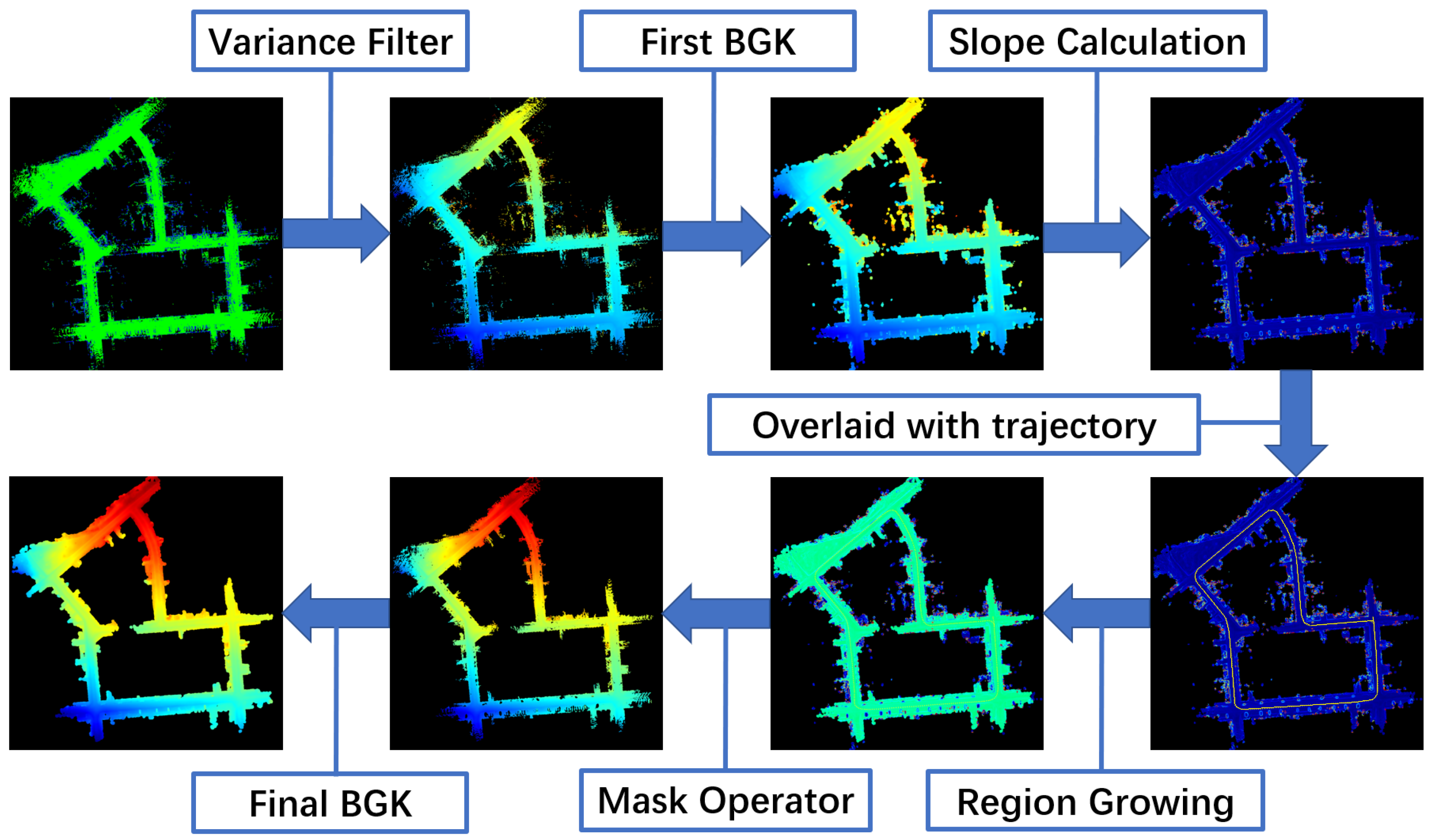
3.1. Terrain Modeling

The goal of terrain modeling is to extract a complete and dense 3D terrain model from a point cloud. In order to achieve this goal, we can either directly process the point cloud map as a whole, or process a single frame of data first, and then perform result-level fusion. This paper adopts the latter approach.

Let ${\mathbf{L}}_i$ denote a LiDAR scan. We first divide it into a ground part ${\mathbf{L}}_i^g$ and a non-ground part ${\mathbf{L}}_i^{ng}$ using any off-the-shelf ground segmentation algorithm [21]. Then we use the LiDAR pose ${\mathbf{Tr}}_{m\_l_i}$ to convert the ground part ${\mathbf{L}}_i^g$ to the map coordinate frame. By assembling all the transformed ${\mathbf{L}}_i^g$ in the map coordinate frame, we get the map ground point cloud ${\mathcal{M}}^g$:

$${\mathcal{M}}^g=\{{\mathbf{Tr}}_{m\_l_i}\ast {\mathbf{L}}_i^g,i=1,2,\cdots ,m\}.$$

(1)

However, any ground segmentation algorithm that only processes a single frame of data may produce false detections. Therefore, the assembled map ground point cloud also has certain errors. In order to eliminate these errors, we designed the following terrain modeling algorithm, as shown in Figure 2, which mainly includes the following steps:

• Preprocess with a variance filter.

We first project the map ground point cloud ${\mathcal{M}}^g$ into a 2D XY grid plane and calculate the mean ${\mu }_j$ and variance ${\sigma }_j^2$ for each grid cell based on all points that fall on that cell. We believe that for a real ground cell, it has a unique elevation value that should not change no matter where the grid cell is viewed from, so its standard deviation $\sigma$ should be small. Therefore, we threshold the standard deviation and treat grid cells with standard deviation less than some threshold $thresh\_std$ as reliable ground cells, while the rest are unreliable cells. By jointly considering grid cell quantization error, pose estimation error, and ranging error of the LiDAR point cloud itself, we set this threshold to 0.1 in all subsequent experiments and did not change it.

• BGK inference with bilateral filtering.

The variance filter enables us to find those unreliable terrain grid cells. In order to obtain a complete and dense terrain model, we must find a suitable estimate for those unreliable cells. To achieve this, we draw inspiration from the recently published terrain estimation algorithm [7], where the terrain to be estimated is considered to be a locally continuous surface and the elevation of any point in the surface can be estimated from adjacent points’ elevation by nonlinear regression. Similar to [7], we use Bayesian generalized kernel (BGK) inference [22] as the nonlinear regression method. To prevent the algorithm from over-smoothing terrain edges, the bilateral filtering method introduced in [7] is also used.

• Region growing on the normal map.

The result of BGK inference is a dense surface, from which the normal direction of each grid cell can be easily calculated [7]. Based on the normal direction, we can also calculate the slope of the terrain. For a grid cell $(u,v)$ in the projected 2D XY grid plane, it can be expressed as a 3D point $\mathbf{p}=[0;0;E(u,v\left)\right]$, where $E(u,v)$ is the estimated elevation from BGK inference. Then its four neighbors in the XY grid plane can be represented as ${\mathbf{p}}_l=[0;-reso;E(u,v-1)]$, ${\mathbf{p}}_r=[0;reso;E(u,v+1)]$, ${\mathbf{p}}_u=[reso;0;E(u-1,v)]$, and ${\mathbf{p}}_d=[-reso;0;E(u+1,v)]$, where $reso$ is the grid resolution. Its normal direction $\mathbf{n}(u,v)$ and slope value can be then calculated as:

$$\left\{\begin{array}{c}\mathbf{n}(u,v)=\mathrm{cross}({\mathbf{p}}_l-{\mathbf{p}}_r,{\mathbf{p}}_u-{\mathbf{p}}_d)\hfill \\ \mathrm{slope}(u,v)=\frac{\pi }{2}-\mathrm{acos}\left(\mathrm{dot}\left(\mathbf{n}\right(u,v),[0;0;1\left]\right)\right)\hfill \end{array}\right.$$

(2)

where $\mathrm{cross}(·)$ and $\mathrm{dot}(·)$ represent the cross product and dot product of two vectors.

Based on the slope angle, we can set another threshold $thresh\_slope$ to determine the traversability region of the vehicle. Following [23], the areas that the vehicle has traversed are all reliable terrain areas. Therefore, we project the vehicle trajectory onto the terrain map and find the corresponding grid cell. These grid cells are considered as terrain seed points. From these seed points, we perform region growing operator. The region stops growing when the slope angle of the grid cells is higher than the threshold $thresh\_slope$. Finally, these regions have been grown from a terrain mask. Only grid cells within this mask are considered as terrain cells. Another BGK inference is then performed on these cells, and the output of the BGK forms the final terrain model.

In Figure 3, we compare the input and output of the proposed terrain modeling approach. It can be seen that, given a noisy input, the proposed algorithm can generate a dense and accurate terrain model.

3.2. Moving Points Identification

Based on the terrain modeling method, we can divide the entire map point cloud into three parts: the noise part below the terrain ${\mathcal{M}}^n$, the terrain part ${\mathcal{M}}^g$, and the obstacle part above the terrain ${\mathcal{M}}^o$. An illustrative example is shown in Figure 4, where ${\mathcal{M}}^n$, ${\mathcal{M}}^g$, and ${\mathcal{M}}^o$ are colored blue, green, and red, respectively. To find moving objects, we are only interested in the obstacle map ${\mathcal{M}}^o$.

In this section, we aim to design a model-free method for moving point identification. We extend the log-odds approach used in the occupancy mapping literature [20,24]. In the log-odds method, each frame of observation is considered to be independent. Multiple observations are then combined in a Bayesian framework. The posterior distribution is used to determine the occupancy state of the grid cell. This idea can be easily extended for the task of moving point identification.

By assuming an equal prior on the dynamic/stationary state, we can simply count the number of times a map point (or the 3D voxel to which the point belongs) has been observed as free or occupied. If the free counter is greater than the occupancy counter, then the point is likely to be a moving point, and vice versa. Due to the efficient implementation in Octomap [20], this method is often used as a baseline in some recently proposed moving object identification methods [3,4,25].

Our method differs from the classic Octomap method [20] in the following ways: First, in the Octomap method, it needs to maintain a 3D voxel map in 3D space. Each frame observation is then projected to the voxel map, and the voxel state is updated using ray-casting operators. In this paper, we deal with the inverse of this problem, i.e., we already have a 3D voxel map and we need to determine which voxels are likely to be dynamic. Instead of projecting each frame onto the map, we back project the map onto each frame and perform a map-to-frame comparison. In this way, we can avoid the quantization error [5,26] that occurs in the Octomap method. Second, when performing map-to-frame comparisons, we use the range image representation for the current frame. The range image representation implicitly models the ray casting operator in Octomap, and it enables us to use projective association instead of nearest neighbor search to find associated points. However, as pointed out in [27], the range image representation also introduces quantization errors. To address this, instead of performing point-to-point comparisons, we compare each projected point to a small neighborhood near the projected pixel.

Essentially, our method can be viewed as a voting method. Each frame can vote on the dynamic/static state of each map point through the map-to-frame comparison. The final state of the map point is determined by all votes. An illustrative example is shown in Figure 5. More specifically, let ${}^M{\mathbf{p}}_k$ denote a point in the obstacle map ${\mathcal{M}}^o$. It is then assigned a static counter $c_k^s$ and a dynamic counter $c_k^d$, which counts the number of times that this point is considered as static or dynamic by each map-to-frame comparison. This map point is first projected to the local frame coordinate based on the frame pose ${\mathrm{Tr}}_{m\_l_i}$:

$${}^{l_i}{\mathbf{p}}_k=\mathrm{inv}\left({\mathrm{Tr}}_{m\_l_i}\right)\ast {}^M{\mathbf{p}}_k$$

(3)

Let ${\mathbf{R}}_i$ denotes the range image representation of the ith LiDAR scan. Its width and height are w and h, respectively. The angle range corresponding to the horizontal direction is $[0,2\pi )$, and the angle range corresponding to the vertical direction is $[{\theta }_{down},{\theta }_{up}]$. For a 3D point ${}^{l_i}{\mathbf{p}}_k=[x_k;y_k;z_k]$, its corresponding range image coordinate $[u,v]$ can be calculated as [28]:

$$\left\{\begin{array}{c}{r}_k=\sqrt{x_k^2+y_k^2+z_k^2}\hfill \\ v=\lfloor ({\theta }_{up}-arcsin(z_k/r_k))/({\theta }_{up}-{\theta }_{down})·h,\hfill \\ u=\lfloor \frac{1}{2}(1+arctan(x_k/y_k)/\pi )·w,\hfill \end{array}\right.$$

(4)

where ⌊·⌋ is the floor operator.

When comparing $r_k$ with the values stored in the range image ${\mathbf{R}}_i(v,u)$, the following cases might occur:

$$\left\{\begin{array}{c}\mathrm{Case}\mathrm{A}:|r_k-{\mathbf{R}}_i(v,u)|<=thresh\_dist\hfill \\ \mathrm{Case}\mathrm{B}:r_k>{\mathbf{R}}_i(v,u)+thresh\_dist\hfill \\ \mathrm{Case}\mathrm{C}:r_k<{\mathbf{R}}_i(v,u)-thresh\_dist\hfill \\ \mathrm{Case}\mathrm{D}:{\mathbf{R}}_i(v,u)isinvalid\hfill \end{array}\right.$$

(5)

where $thresh\_dist$ is a distance threshold. Among the four cases defined in Equation (5), Case A indicates that a close-by point to the map point ${}^M{\mathbf{p}}_k$ can be found in the current frame. Therefore, the static counter of this map point should be increased by 1. Case B suggests that the map point is located in the occluded area of the current observation, so no information about whether the map point is moving or static can be inferred from this observation. Case C suggests that the map point locates nearer than the current observation, thus producing a strong motion evidence. The dynamic counter for the map point should be increased by 1. Case D simply suggests that there are no corresponding observations in the current frame. Therefore, no evidence of movement/static can be provided.

Just as pointed out in [28], different types of LiDAR devices may contain non-uniformly distributed longitudinal resolutions. If the longitudinal angle is equally divided as in Equation (4), it will bring a large quantization error. To decrease the quantization errors, the height of the range image needs to be increased. A side effect of increasing the height is that the range image will contain more empty areas, i.e., Case D in Equation (5) will appear more frequently.

To overcome this problem, instead of only comparing $r_k$ with ${\mathbf{R}}_i(v,u)$, it is compared with a small neighborhood $\left\{{\mathbf{R}}_i(v+\Delta v_j,u+\Delta u_j)\right\}$ around ${\mathbf{R}}_i(v,u)$. The following strategy is then used to fuse the comparison results: as long as Case A appears once in all comparison results, it is finally judged as Case A, that is, the static counter of the map point is increased by 1. When part of the comparison results are Case C, and the rest are Case D, the final judgment is set to Case C, and the dynamic counter will be increased by 1. Otherwise, the static and dynamic counters remain unchanged.

The map point cloud is projected to each frame and the map-to-frame is performed separately. The comparison results are fused in the static counter and dynamic counter. After all the comparisons, if the static counter is greater than the dynamic counter, the point is considered static, otherwise it is considered as a dynamic point. The entire algorithm is summarized in Algorithm 1.

Algorithm 1 Moving Point Identification

1: Input: Obstacle Map Point Cloud ${\mathcal{M}}^o=\{{}^M{\mathbf{p}}_k,k=1,2,\cdots n\}$, LiDAR scans $\{{\mathbf{L}}_i,i=1,2,\cdots ,m\}$ with associated range image representation $\left\{{\mathbf{R}}_i\right\}$ and poses relative to the map ${\mathrm{Tr}}_{m\_l_i}$; 2: Output: Dynamic Map Point Cloud ${\mathcal{M}}^{do}$ and Static Map Point Cloud ${\mathcal{M}}^{so}$; 3: Initialize ${\mathcal{M}}^{do}$ and ${\mathcal{M}}^{so}$ to empty set; 4: Assign each map point ${}^M{\mathbf{p}}_k$ a static counter $c_k^s$ and a dynamic counter $c_k^d$ which are initialized to 0; 5: for k=1:n do 6:     for i=1:m do 7:         Transform map point ${}^M{\mathbf{p}}_k$ from map coordinate to local LiDAR coordinate ${}^{l_i}{\mathbf{p}}_k$ using Equation (3). 8:         Calculate the range image coordinate $[v,u]$ for ${}^{l_i}{\mathbf{p}}_k$ using Equation (4). 9:         for $(\Delta v,\Delta u)\in \{\Delta v_j,\Delta u_j\}$ do 10:            Compare $r_k=\parallel {}^{l_i}{\mathbf{p}}_k\parallel$ with ${\mathbf{R}}_i(v+\Delta v,u+\Delta u)$ using Equation (5) and obtain the Comparison Result. 11:            if Comparison Result == Case A then 12:                Fused Result = Case A 13:                break; 14:            else 15:                if Comparison Result == Case C or Case D then 16:                    Fused Result = Case C 17:                else 18:                    Fused Result = Otherwise 19:                    break; 20:                end if 21:            end if 22:         end for 23:         if Fused result == Case A then 24:            $c_k^s=c_k^s+1$ 25:         else 26:            if Fused result == Case C then 27:                $c_k^d=c_k^d+1$ 28:            end if 29:         end if 30:     end for 31:     if $c_k^s>=c_k^d$ then 32:         ${\mathcal{M}}^{so}\to \{{\mathcal{M}}^{so},{}^M{\mathbf{p}}_k\}$ 33:     else 34:         ${\mathcal{M}}^{do}\to \{{\mathcal{M}}^{do},{}^M{\mathbf{p}}_k\}$ 35:     end if 36: end for

4. Results and Discussion

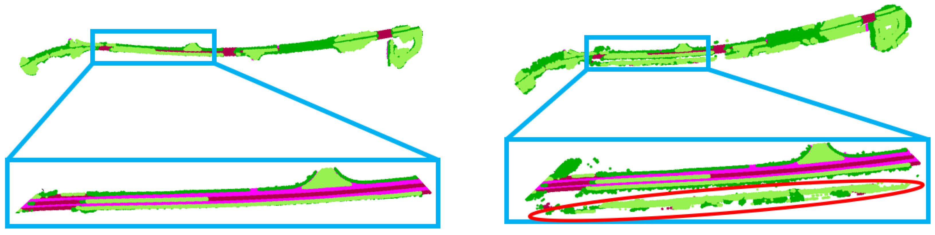
4.1. Evaluation on the Terrain Modeling Approach

The proposed approach is quantitatively evaluated on the publicly available SemanticKITTI dataset. We first conduct experiments to evaluate the performance of the proposed terrain modeling approach. We choose to use PatchWork [21] as our single-frame ground segmentation algorithm. This approach is a fast algorithm and performs reasonably well on the SemanticKITTI dataset.

To assemble frames together, we can directly use the poses provided by the SemanticKITTI dataset. These poses are generated by the SuMa algorithm [29]. Upon closer inspection of the poses, we noticed that there exist some errors in the poses, mainly in the loop closure scenario. For example, Figure 6 shows three examples when overlaying two frames using the SuMa poses. Therefore, we recompute the pose using our own mapping method developed in [2]. The generated poses are mostly consistent with SuMa poses, but differ slightly in loop closure scenarios.

Regarding parameters, we set $thresh\_std=0.1$ m, $thresh\_slope=15$ degrees, and $thresh\_dist=0.5$ m. The width and height of the range image are set to 1080 and 128, respectively.

The terrain modeling method is performed on five SemanticKITTI sequences (00, 01, 02, 05, and 07), and the results are shown in Figure 7.

To quantitively evaluate the accuracy of terrain modeling, we use semantic labels provided in the SemanticKITTI dataset. Following [21], semantic classes including lane marking, road, parking, sidewalk, other ground, terrain, and vegetation (only points with a z-value below −1.3 m) are considered as the ground truth for terrain modeling. Precision and recall are used as performance metrics. The results are shown in

Table 1. Terrain modeling results on the SemanticKITTI dataset. The best results are colored in bold.

Sequence	Approach	Precision [%]	Recall [%]	F1-Measure
00	Patchwork [21]	72.94	92.00	0.8137
	Ours	94.78	78.20	0.8570
01	Patchwork [21]	89.96	80.94	0.8521
	Ours	98.40	69.25	0.8129
02	Patchwork [21]	82.27	93.72	0.8763
	Ours	97.80	85.18	0.9105
05	Patchwork [21]	72.64	94.67	0.8221
	Ours	92.10	85.19	0.8851
07	Patchwork [21]	71.92	92.03	0.8074
	Ours	99.30	78.67	0.8778

.

The results of Patchwork in Table 1 differ slightly from those reported in [21]. In [21], the results are evaluated frame by frame, whereas in our case the performance is evaluated at the map level for the whole sequence. As can be seen from Table 1, our method outperforms Patchwork in all sequences except Sequence 01. Our method consistently achieves high accuracy but relatively low recall. The reason is simply because our method considers the reachability of the terrain and thus includes a region growing operator. Figure 8 shows the comparison between the results obtained by our method and the ground truth for Sequence 01. It can be observed that the ground truth also contains most of the terrain located outside the main roads, and these regions are considered unreachable by the region growing operator, so they are not treated as terrain in our method, resulting in relatively low recall.

Finally, it is important to point out that the aim of our terrain modeling approach is to obtain a dense and continuous terrain on which moving objects typically stand. Modeling terrain with high accuracy can help us segment moving objects well. For areas not covered by the terrain model, they can all be treated as potential moving objects, and directly sent to our moving points identification module.

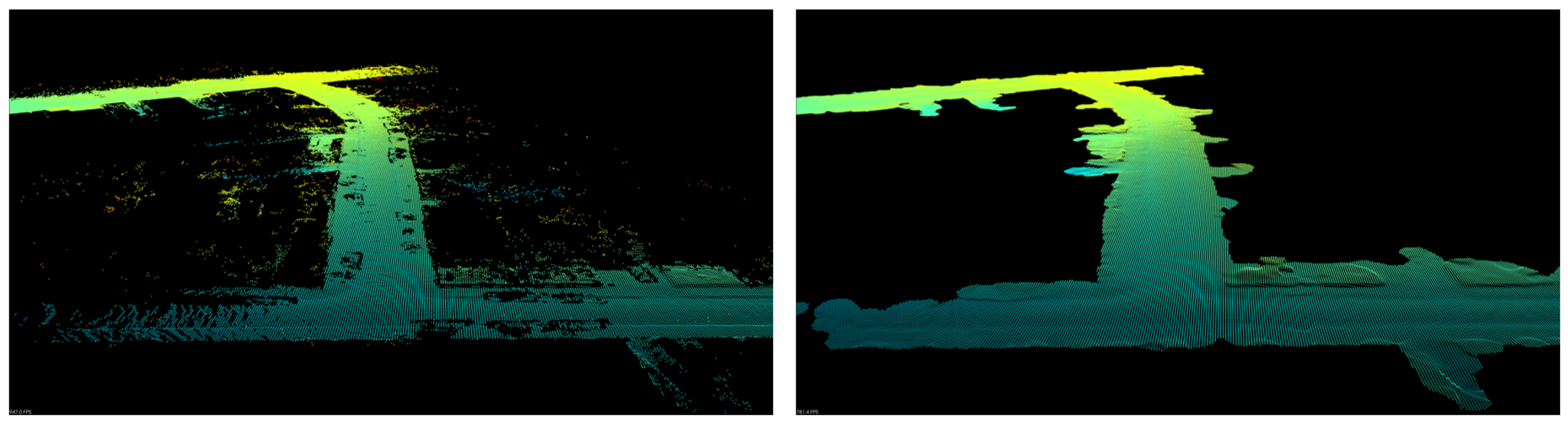
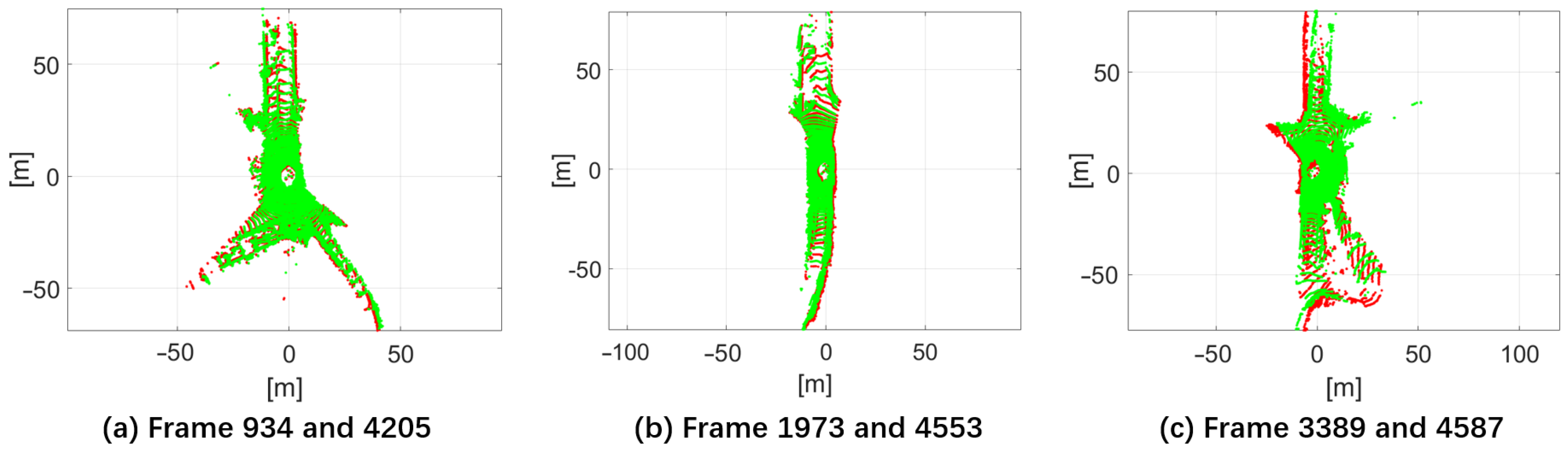
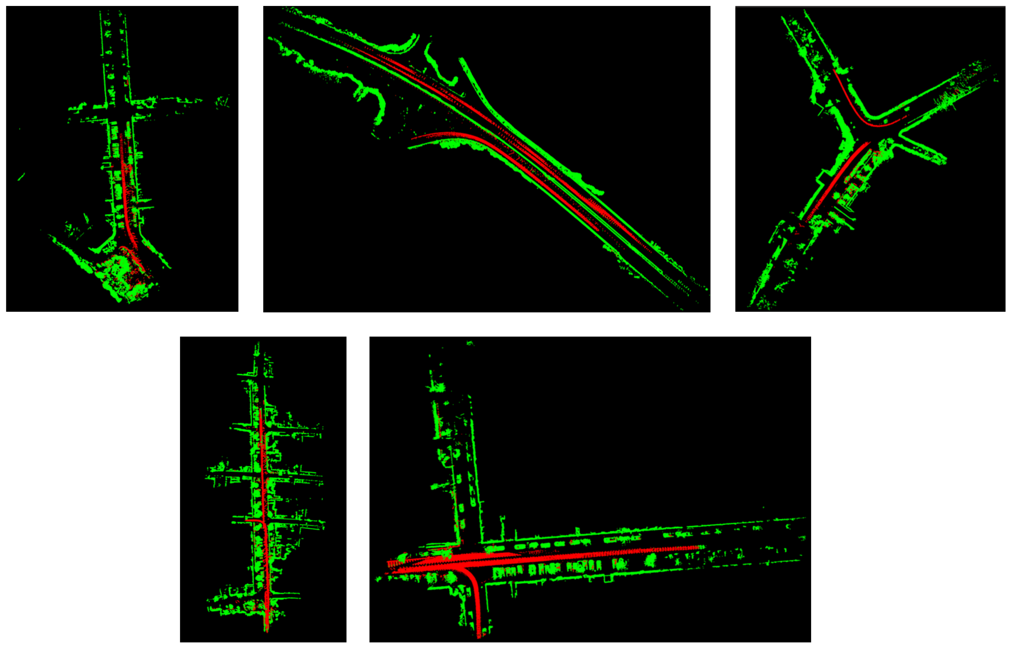
4.2. Evaluation on the Map Cleaning Performance

To evaluate the performance of the entire map cleaning algorithm, we follow the experimental protocol in [4]. Points belonging to semantic classes 252, 253, 254, 255, 256, 257, 258, and 259 form the dynamic point set. The remaining points form the static point set. Experiments are conducted on five subsets of SemanticKITTI datasets, including sequence 00 (4390–4530), 01(150–250), 02(860,950), 05(2350,2670), and 07(630–820).

The width and height of the range image are set to 1080 and 256, respectively. As shown in [28], setting the range image height to a larger value is beneficial for maintaining a low range image quantization error. We directly use the terrain modeling results generated in the previous terrain modeling experiment. The points above the terrain constitute the Obstacle Point Cloud Map ${\mathcal{M}}^o$. For regions not covered by the terrain model, they are directly added to ${\mathcal{M}}^o$ to enable a more fair comparison with state-of-the-art approaches. The moving points identification algorithm detailed in Algorithm 1 is applied on ${\mathcal{M}}^o$.

The results for the five SemanticKITTI sequences are shown in Figure 9, where moving points are colored in red and static points are colored in green. It can be observed that most of the long tails generated by moving objects are correctly identified by the proposed approach.

To quantitatively assess the performance of the proposed method, we choose to use preservation rate (PR) and rejection rate (RR) proposed in [4] as performance measures. Compared with the commonly used precision and recall, these two metrics are more sensitive for moving points identification and thus more suitable for our scenario. Quantitative results and comparisons with state-of-the-art approaches are shown in

Table 2. Map cleaning results on the SemanticKITTI dataset. The best results are colored in bold.

Sequence	Approach	PR [%]	RR [%]	${\mathit{F}}_1$ Score
00	Octomap [20]	76.73	99.12	0.865
	Peopleremover [5]	37.52	89.12	0.528
	Removert [3]	85.50	99.35	0.919
	ERASOR [4]	93.98	97.08	0.955
	Ours	98.89	98.18	0.9853
01	Octomap [20]	53.16	99.66	0.693
	Peopleremover [5]	94.22	93.61	0.939
	Removert [3]	85.50	99.35	0.919
	ERASOR [4]	91.48	95.38	0.934
	Ours	99.74	94.98	0.9730
02	Octomap [20]	54.11	98.77	0.699
	Peopleremover [5]	29.04	94.53	0.444
	Removert [3]	76.32	96.79	0.853
	ERASOR [4]	87.73	97.01	0.921
	Ours	99.37	99.03	0.9920
05	Octomap [20]	76.34	96.78	0.854
	Peopleremover [5]	38.49	90.63	0.540
	Removert [3]	86.90	87.88	0.874
	ERASOR [4]	88.73	98.26	0.933
	Ours	99.14	97.92	0.9852
07	Octomap [20]	77.84	96.94	0.863
	Peopleremover [5]	34.77	91.98	0.505
	Removert [3]	80.69	98.82	0.888
	ERASOR [4]	90.62	99.27	0.948
	Ours	98.98	97.25	0.9811

.

As can be seen from Table 2, our proposed method outperforms state-of-the-art approaches on all five test sequences. Although our method is in principle analogous to Octomap [20], we outperform it by a large margin. The reasons for this should be attributed to our principled approach that combines the merits of terrain modeling, map-frame comparison, and range image utilization. Figure 10 also compares the errors that occurred in our approach and in ERASOR [4]. It can be seen that our method produces many fewer false positives than ERASOR.

After carefully inspecting the false detections occurred in our approach, we noticed that some of these errors were caused by possibly erroneous intra-frame compensation of the raw LiDAR scan. As noticed in [29], the original poses associated with the KITTI odometry dataset are not accurate. Every LiDAR scan in this dataset has been motion compensated based on these inaccurate poses. Therefore, errors may appear in the compensated LiDAR point cloud. Figure 11 shows a zoomed-in view of our results in Figure 10. The area enclosed by the yellow ellipse should correspond to one wall, but three walls appear in the picture, probably due to an intra-frame compensation error. In future work, we plan to find the raw LiDAR scans corresponding to the SemanticKITTI dataset and use our corrected poses to perform intra-frame compensation. Care should be taken if the semantic labels provided in SemanticKITTI can be seamlessly transferred to the original scan.

We also evaluated the running time of MapCleaner. For the terrain modeling part, it takes approximately 7.3 s, 17.6 s, 14.7 s, 5.1 s, and 2.1 s to process sequence 00, 01, 02, 05, and 07, respectively. For the map cleaning part, it takes around 3.6 s to process the subset of sequence 07, which contains a total of 190 frames (frame 630–820). On average, it takes only 18.94 ms to process a single frame (perform map-to-frame comparison).

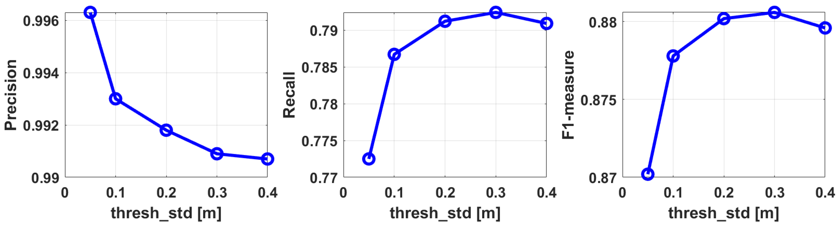
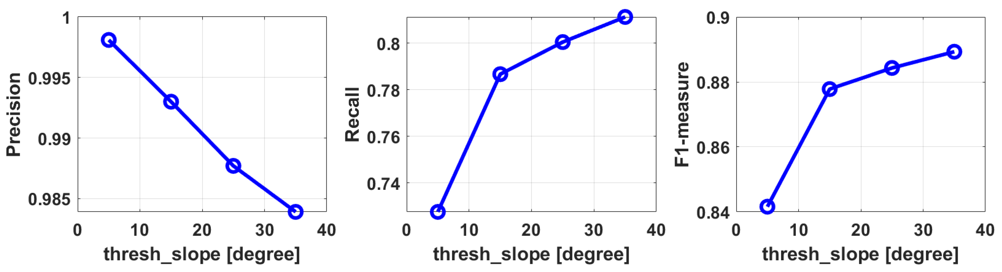
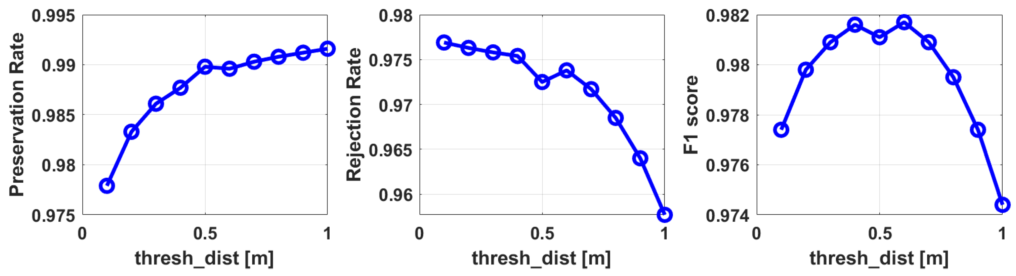
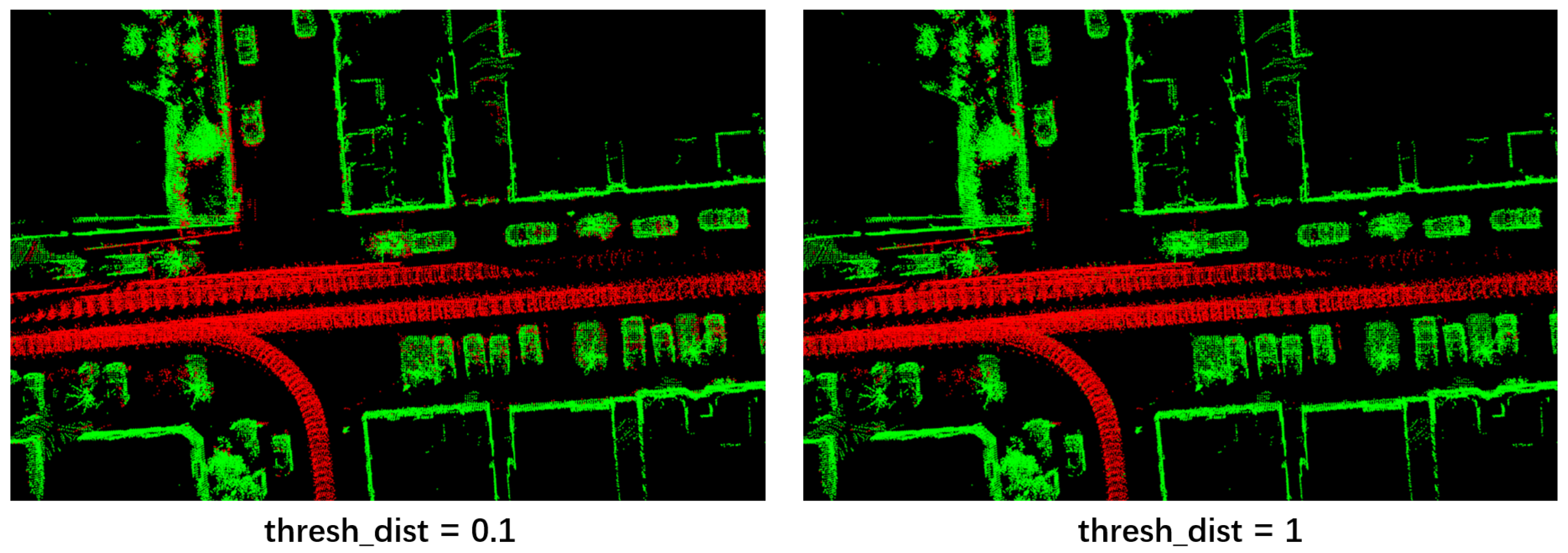
4.3. Ablation Studies

We now present the ablation studies of our method. The proposed method has a total of three parameters, namely $thresh\_std$ for the variance filter, $thresh\_slope$ for determining the slope angle of the traversable region, and $thresh\_dist$ used in (5). Whereas $thresh\_std$ and $thresh\_slope$ are related to terrain modeling, $thresh\_dist$ is directly related to the map cleaning performance.

For $thresh\_std$, it represents the standard deviation of the ground height value for each grid cell. In Figure 12, we visualize this value for all grid cells in the SemanticKITTI sequence 07 dataset. We change $thresh\_std$ to different values and recalculate precision, recall, and F1-measure. The results are shown in Figure 13. It can be observed that, with an increased value of $thresh\_std$, the precision rate decreases. The F1-measure does not change too much when $thresh\_std$ is set between 0.1 and 0.4. Therefore, we choose to set $thresh\_std$ to 0.1 for better precision.

After fixing $thresh\_std$ to 0.1, we also changed $thresh\_slope$ to different values. The terrain modeling accuracy is shown in Figure 14, and a similar trend to that in Figure 13 can be observed: as the value of $thresh\_slope$ increases, the precision rate decreases and the recall rate increases. Although setting $thresh\_slope$ to 35 degrees produces a slightly larger F1-measure, we still prefer to set it to 15 degrees. A comparison example is shown in Figure 15. Setting $thresh\_slope$ to 15 degrees may produce smoother terrain without sudden changes compared to 35 degrees. In addition, the climbing ability of most vehicles is around 15 degrees, we therefore set $thresh\_slope$ to 15 degrees in this paper.

The parameter $thresh\_dist$ is directly related to map cleaning performance. We change this value from 0.1 to 1 and evaluate map cleaning performance on the SemanticKITTI sequence 07 dataset. The preservation rate, rejection rate, and F1 score under different $thresh\_dist$ values are shown in Figure 16. A larger $thresh\_dist$ value will produce a higher preservation rate and a lower rejection rate. Two comparative examples are shown in Figure 17. From the figure, we can observe that smaller $thresh\_dist$ value produce more false positives. Finally, we chose to set $thresh\_dist$ to 0.5 in all experiments.

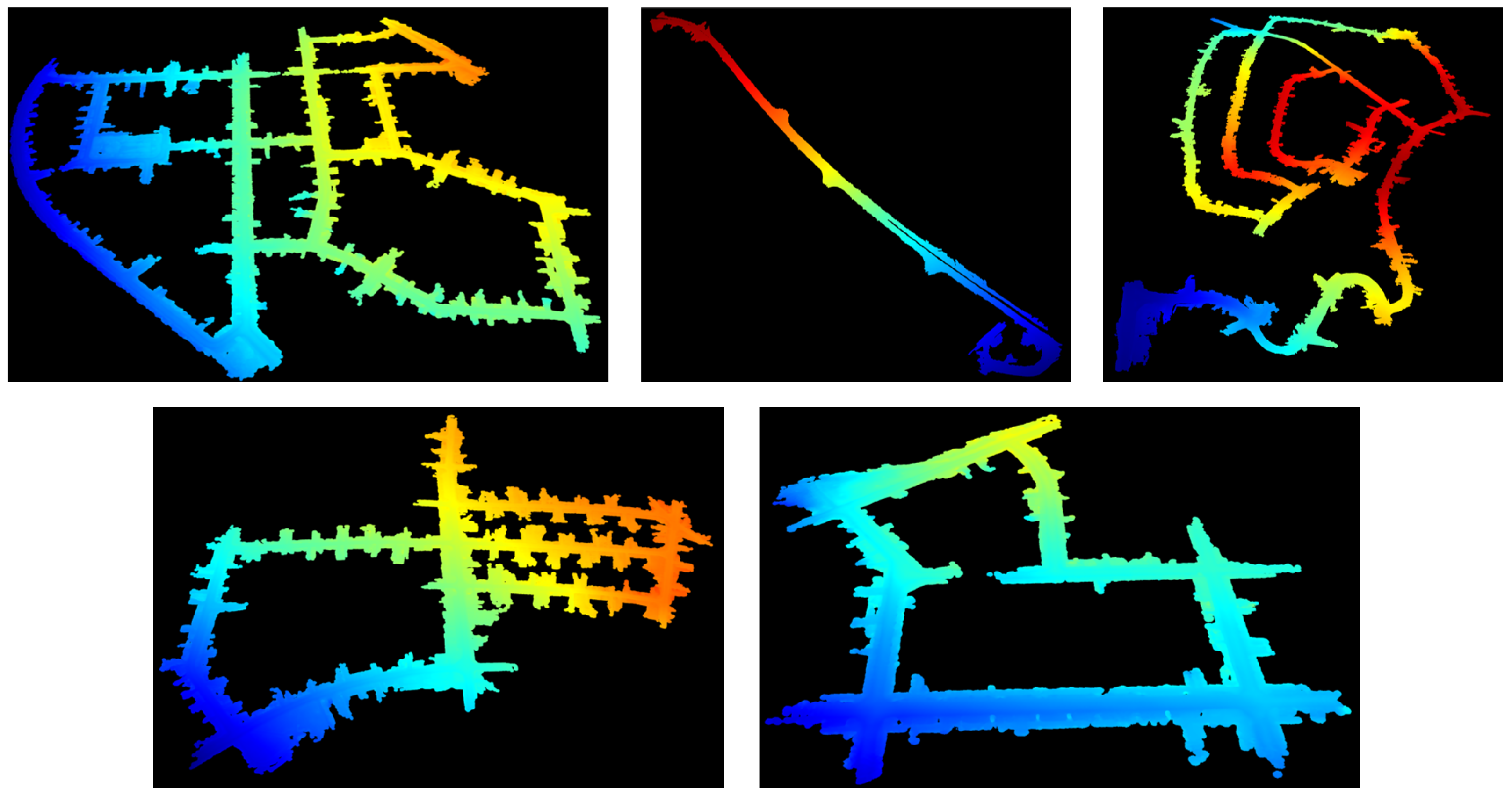
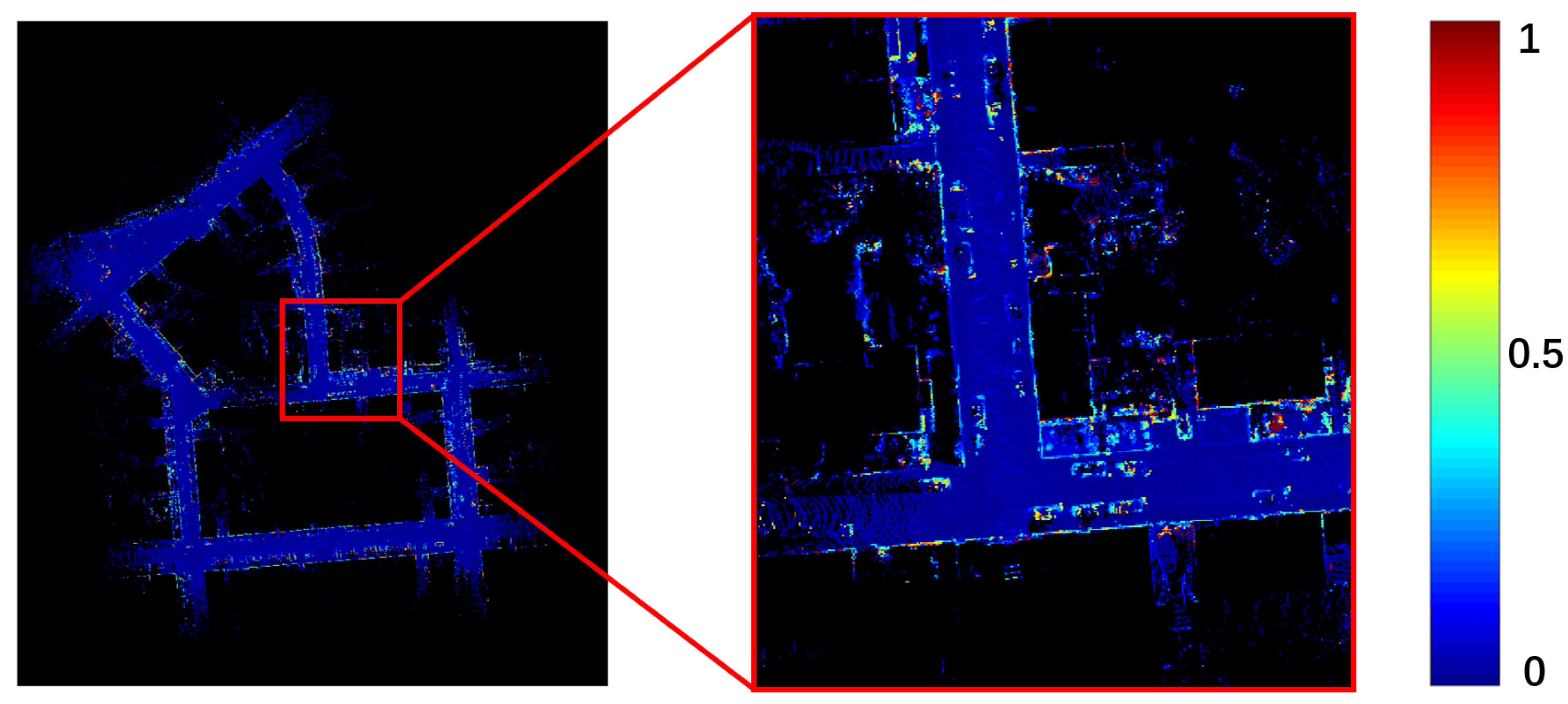
4.4. Experiments on Our Dataset

In addition to the SemanticKITTI dataset, we also evaluate MapCleaner on a dataset collected by our own vehicle. As shown in Figure 18, the vehicle is equipped with a Robosense Ruby 128-channel LiDAR [28]. The vertical resolution of this LiDAR is quite different from the LiDAR (Velodyne 64) used in the SemanticKITTI dataset.

To apply MapCleaner to our own dataset, we simply change the range image width and height to 2160 and 256, respectively. Other parameters, including $thresh\_std$, $thresh\_slope$, and $thresh\_dist$, are set to the same values used in the SemanticKITTI dataset. The map cleaning results are also shown in Figure 18. It can be observed that MapCleaner successfully removes long trails of dynamic objects in the original map. This confirms the applicability of MapCleaner to different types of LiDAR devices.

5. Concluding Remarks

In this paper, we propose MapCleaner, an efficient map cleaning algorithm that can remove moving objects from a map point cloud. MapCleaner is mainly composed of two modules: a terrain modeling module and a moving point identification module. We emphasize that terrain modeling should be a pre-step for map cleaning, as almost all the moving objects stand on the ground. We then propose a novel approach that can estimate a dense and accurate terrain model from the map point cloud. For the moving point identification module, we follow a similar idea to Octomap, but make several improvements, including the map-to-frame comparison and the utilization of range image. Experiments are conducted on the SemanticKITTI dataset, and experimental results show that our proposed method outperforms state-of-the-art methods in both terrain modeling accuracy and map cleaning accuracy. Our method achieves almost perfect F1 scores (0.9920 on sequence 02) on some SemanticKITTI sequences. We also analyze potential errors in the SemanticKITTI dataset. Errors arise not only in inaccurate poses, but also in erroneous intra-frame compensation in the original KITTI odometry dataset. Future work will try to correct these errors for fairer evaluations.

Compared with existing methods, the proposed MapCleaner only needs to adjust a few parameters and is easily adaptable to other types of LiDAR devices. We also evaluate it on our own dataset collected by a Robosense Ruby 128-channel LiDAR. Qualitative results show that MapCleaner successfully removes most moving objects without fine-tuning parameters.

References

1. Fu, H.; Yu, R.; Wu, T.; Ye, L.; Xu, X. An Efficient Scan-to-Map Matching Approach based on Multi-channel Lidar. J. Intell. Robot. Syst. 2018, 91, 501–513. [Google Scholar] [CrossRef]
2. Ren, R.; Fu, H.; Xue, H.; Sun, Z.; Ding, K.; Wang, P. Towards a fully automated 3d reconstruction system based on lidar and gnss in challenging scenarios. Remote Sens. 2021, 13, 1981. [Google Scholar] [CrossRef]
3. Kim, G.; Kim, A. Remove, then revert: Static point cloud map construction using multiresolution range images. In Proceedings of the IEEE International Conference on Intelligent Robots and Systems, Las Vegas, NV, USA, 24 October 2020–24 January 2021; pp. 10758–10765. [Google Scholar]
4. Lim, H.; Hwang, S.; Myung, H. ERASOR: Egocentric Ratio of Pseudo Occupancy-Based Dynamic Object Removal for Static 3D Point Cloud Map Building. IEEE Robot. Autom. Lett. 2021, 6, 2272–2279. [Google Scholar] [CrossRef]
5. Schauer, J.; Nuchter, A. The Peopleremover-Removing Dynamic Objects from 3-D Point Cloud Data by Traversing a Voxel Occupancy Grid. IEEE Robot. Autom. Lett. 2018, 3, 1679–1686. [Google Scholar] [CrossRef]
6. Chen, X.; Mersch, B.; Nunes, L.; Marcuzzi, R.; Vizzo, I.; Behley, J.; Stachniss, C. Automatic Labeling to Generate Training Data for Online LiDAR-Based Moving Object Segmentation. IEEE Robot. Autom. Lett. 2020, 7, 6107–6114. [Google Scholar] [CrossRef]
7. Xue, H.; Fu, H.; Ren, R.; Zhang, J.; Liu, B.; Fan, Y.; Dai, B. LiDAR-based Drivable Region Detection for Autonomous Driving. In Proceedings of the IEEE International Conference on Intelligent Robots and Systems, Prague, Czech Republic, 27 September–1 October 2021; pp. 1110–1116. [Google Scholar]
8. Chen, C.; Yang, B. Dynamic occlusion detection and inpainting of in situ captured terrestrial laser scanning point clouds sequence. ISPRS J. Photogramm. Remote. Sens. 2016, 119, 90–107. [Google Scholar] [CrossRef]
9. Gehrung, J.; Hebel, M.; Arens, M.; Stilla, U. An approach to extract moving objects from MLS data using a volumetric background representation. ISPRS Ann. Photogramm. Remote. Sens. Spatial Inf. Sci. 2017, 4, 107–114. [Google Scholar] [CrossRef]
10. Fang, J.; Zhou, D.; Yan, F.; Zhao, T.; Zhang, F.; Ma, Y.; Wang, L.; Yang, R. Augmented LiDAR simulator for autonomous driving. IEEE Robot. Autom. Lett. 2020, 5, 1931–1938. [Google Scholar] [CrossRef]
11. Baur, S.A.; Emmerichs, D.J.; Moosmann, F.; Pinggera, P.; Ommer, B.; Geiger, A. SLIM: Self-Supervised LiDAR Scene Flow and Motion Segmentation. In Proceedings of the IEEE International Conference on Computer Vision (ICCV), Montreal, QC, Canada, 10–17 October 2021; pp. 13106–13116. [Google Scholar]
12. Pang, Z.; Li, Z.; Wang, N. Model-free Vehicle Tracking and State Estimation in Point Cloud Sequences. In Proceedings of the IEEE International Conference on Intelligent Robots and Systems, Prague, Czech Republic, 27 September–1 October 2021; pp. 8075–8082. [Google Scholar]
13. Vatavu, A.; Rahm, M.; Govindachar, S.; Krehl, G.; Mantha, A.; Bhavsar, S.R.; Schier, M.R.; Peukert, J.; Maile, M. From Particles to Self-Localizing Tracklets: A Multilayer Particle Filter-Based Estimation for Dynamic Grid Maps. IEEE Intell. Transp. Syst. Mag. 2020, 12, 149–168. [Google Scholar] [CrossRef]
14. Fan, T.; Shen, B.; Chen, H.; Zhang, W.; Pan, J. DynamicFilter: An Online Dynamic Objects Removal Framework for Highly Dynamic Environments. In Proceedings of the 2022 IEEE International Conference on Robotics and Automation (ICRA), Philadelphia, PA, USA, 23–27 May 2020; pp. 7988–7994. [Google Scholar]
15. Yoon, D.; Tang, T.; Barfoot, T. Mapless online detection of dynamic objects in 3D lidar. In Proceedings of the 2019 16th Conference on Computer and Robot Vision, CRV 2019, Kingston, QC, Canada, 29–31 May 2019; pp. 113–120. [Google Scholar]
16. Chen, X.; Li, S.; Mersch, B.; Wiesmann, L.; Gall, J.; Behley, J.; Stachniss, C. Moving Object Segmentation in 3D LiDAR Data: A Learning-based Approach Exploiting Sequential Data. IEEE Robot. Autom. Lett. 2021, 6, 6529–6536. [Google Scholar] [CrossRef]
17. Behley, J.; Garbade, M.; Milioto, A.; Behnke, S.; Stachniss, C.; Gall, J.; Quenzel, J. SemanticKITTI: A dataset for semantic scene understanding of LiDAR sequences. In Proceedings of the IEEE/CVF International Conference on Computer Vision (ICCV), Seoul, Korea, 27 October–2 November 2019. [Google Scholar]
18. Peng, K.; Fei, J.; Yang, K.; Roitberg, A.; Zhang, J.; Bieder, F.; Heidenreich, P.; Stiller, C.; Stiefelhagen, R. MASS: Multi-Attentional Semantic Segmentation of LiDAR Data for Dense Top-View Understanding. IEEE Trans. Intell. Transp. Syst. 2022, 1–16. [Google Scholar] [CrossRef]
19. Zhou, B.; Krähenbühl, P. Cross-view Transformers for real-time Map-view Semantic Segmentation. In Proceedings of the IEEE/CVF Conference on Computer Vision and Pattern Recognition, Seattle, WA, USA, 13–19 June 2020; pp. 13760–13769. [Google Scholar]
20. Wurm, K.M.; Hornung, A.; Bennewitz, M.; Stachniss, C.; Burgard, W. OctoMap: A Probabilistic, Flexible, and Compact 3D Map Representation for Robotic Systems. In Proceedings of the International Conference on Robotics and Automation (ICRA), Paris, France, 31 May–31 August 2020. [Google Scholar]
21. Lim, H.; Oh, M.; Myung, H. Patchwork: Concentric Zone-Based Region-Wise Ground Segmentation with Ground Likelihood Estimation Using a 3D LiDAR Sensor. IEEE Robot. Autom. Lett. 2021, 6, 6458–6465. [Google Scholar] [CrossRef]
22. Shan, T.; Wang, J.; Englot, B.; Doherty, K. Bayesian Generalized Kernel Inference for Terrain Traversability Mapping. In Proceedings of the 2nd Conference on Robot Learning, Zurich, Switzerland, 29–31 October 2018; pp. 829–838. [Google Scholar]
23. Forkel, B.; Kallwies, J.; Wuensche, H.J. Probabilistic Terrain Estimation for Autonomous Off-Road Driving. In Proceedings of the IEEE International Conference on Robotics and Automation, Xi’an, China, 30 May–5 June 2021; pp. 13864–13870. [Google Scholar]
24. Thrun, S. Learning Occupancy Grid Maps with Forward Sensor Models. Auton. Robot. 2003, 15, 111–127. [Google Scholar] [CrossRef]
25. Fu, H.; Xue, H.; Ren, R. Fast Implementation of 3D Occupancy Grid for Autonomous Driving. In Proceedings of the 2020 12th International Conference on Intelligent Human-Machine Systems and Cybernetics, IHMSC 2020, Hangzhou, China, 22–23 August 2020; Volume 2, pp. 217–220. [Google Scholar]
26. Roldão, L.; De Charette, R.; Verroust-Blondet, A. A Statistical Update of Grid Representations from Range Sensors. arXiv 2018, arXiv:1807.08483. [Google Scholar]
27. Fu, H.; Xue, H.; Hu, X.; Liu, B. Lidar data enrichment by fusing spatial and temporal adjacent frames. Remote Sens. 2021, 13, 3640. [Google Scholar] [CrossRef]
28. Wu, T.; Fu, H.; Liu, B.; Xue, H.; Ren, R.; Tu, Z. Detailed analysis on generating the range image for lidar point cloud processing. Electronics 2021, 10, 1224. [Google Scholar] [CrossRef]
29. Behley, J.; Stachniss, C. Efficient Surfel-Based SLAM using 3D Laser Range Data in Urban Environments. Robot. Sci. Syst. 2018, 2018, 59. [Google Scholar]
Figure 1. The left image shows the original point cloud map, where moving cars leave long trails on the map. The right image shows the result after running the proposed MapCleaner on the left image, where most of the moving objects are removed. Points are colored according to the height value.
Remotesensing 14 04496 g001
Figure 2. The flowchart of the proposed terrain modeling approach. From top left to bottom left, points are colored according to variance, height, height, slope, slope, region mask, height and height respectively.
Remotesensing 14 04496 g002
Figure 3. The input and output of the proposed terrain modeling approach. Points are colored according to the height value.
Remotesensing 14 04496 g003
Figure 4. Based on the terrain modeling result, the map point cloud is divided into the noise part below the terrain M n (shown in blue), the terrain part M g (shown in green), and the obstacle point cloud above the terrain M o (shown in red).
Remotesensing 14 04496 g004
Figure 5. The obstacle point cloud map is projected into the local coordinates of each frame and compared with the range image representation (shown in subfigure (a)) of each frame. The comparison results (shown in subfigure (b)) are then combined to obtain the final result (shown in subfigure (c)). In subfigures (b,c), the moving points are colored in red, and the static points are colored in green.
Remotesensing 14 04496 g005
Figure 6. Overlaying two LiDAR frames in Sequence 02 according to the poses provided in the SemanticKITTI dataset. It can be seen that the pose is inaccurate, as the two scans (colored in red and green, respectively) are not well aligned.
Remotesensing 14 04496 g006
Figure 7. The terrain models generated for the five sequences (00, 01, 02, 05, and 07) in the SemanticKITTI dataset. Points are colored according to the height value.
Remotesensing 14 04496 g007
Figure 8. The left figure shows the terrain modeling results from the proposed method on Sequence 01, and the right figure shows the ground truth. It can be seen that the ground truth contains terrain outside the main road. These areas are considered unreachable to vehicles, so they are not modeled by the proposed approach, thus resulting in a relatively low recall. The points are colored according to the semantic lables.
Remotesensing 14 04496 g008
Figure 9. The map cleaning results for the five sequences (00, 01, 02, 05, and 07) in the SemanticKITTI dataset. The identified moving points are colored in red, and the static points are colored in green.
Remotesensing 14 04496 g009
Figure 10. The left two figures shows the errors that occurred in ERASOR, whereas the right shows the errors in our approach. The true positives, true negatives, false positives, and false negatives are colored in green, gray, red, and blue, respectively.
Remotesensing 14 04496 g010
Figure 11. Regions enclosed by the yellow ellipse should correspond to a wall, but three walls appear in the figure, possibly due to the wrong intra-frame compensation of the original LiDAR scan.
Remotesensing 14 04496 g011
Figure 12. The standard deviation value for each grid cell in the SemanticKITTI sequence 07 dataset.
Remotesensing 14 04496 g012
Figure 13. Terrain modeling accuracy on the SemanticKITTI sequence 07 dataset by setting t h r e s h _ s t d to different values.
Remotesensing 14 04496 g013
Figure 14. Terrain modeling accuracy on the SemanticKITTI sequence 07 dataset by setting t h r e s h _ s l o p e to different values.
Remotesensing 14 04496 g014
Figure 15. Terrain modeling results by setting t h r e s h _ s l o p e to different values.
Remotesensing 14 04496 g015
Figure 16. Map cleaning performance under different t h r e s h _ d i s t values.
Remotesensing 14 04496 g016
Figure 17. Moving points identification results by setting t h r e s h _ d i s t to different values. The red points are those identified moving points. The static points are colored in green.
Remotesensing 14 04496 g017
Figure 18. The left figure shows our own experimental platform equipped with a Robosense Ruby 128-channel LiDAR. The middle figure shows the original map, and the right figure shows the map cleaning results by the proposed method. Points are colored based on the height value.
Remotesensing 14 04496 g018