
Validation of Remote-Sensing Algorithms for Diffuse Attenuation of Downward Irradiance Using BGC-Argo Floats


Abstract
:1. Introduction
2. Materials and Methods
2.1. Bio-Argo Data
2.1.1. Retrieval of BGC-Argo Data
2.1.2. Processing of BGC-Argo Data
2.1.3. Computation of the Diffuse Attenuation Coefficients
2.2. Additional Data
2.3. Regional Analysis
2.4. Satellite Data Products
Quality Control of the Satellite Derived Spectra
2.5. Algorithms Tested
2.5.1. Explicit Empirical Algorithms
2.5.2. Lee’s Semi-Analytical Algorithm
2.5.3. Jamet’s Neural Network Algorithm
2.6. PAR Algorithms
2.7. Statistical Performance Metrics
3. Results
3.1. : Global Scale Match-Ups
3.2. : Global Scales Matchups
3.3. Variability in Performance between Satellite Sensors
3.4. Regional Analysis
4. Discussion
4.1. Observed Biases in
4.2. Limitation of Datasets Used to Train Empirical Algorithm
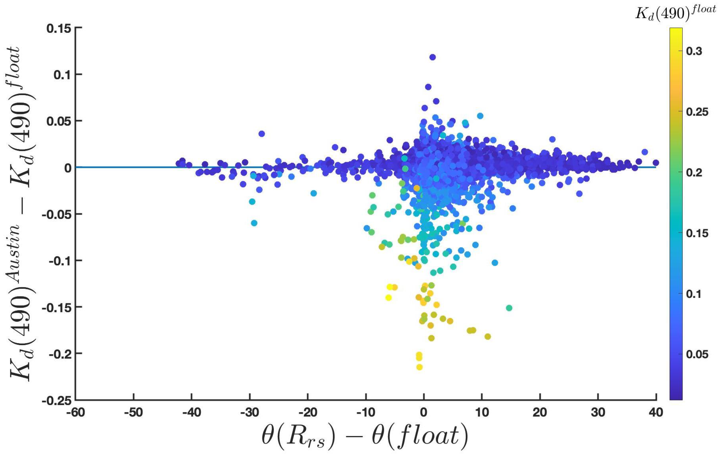
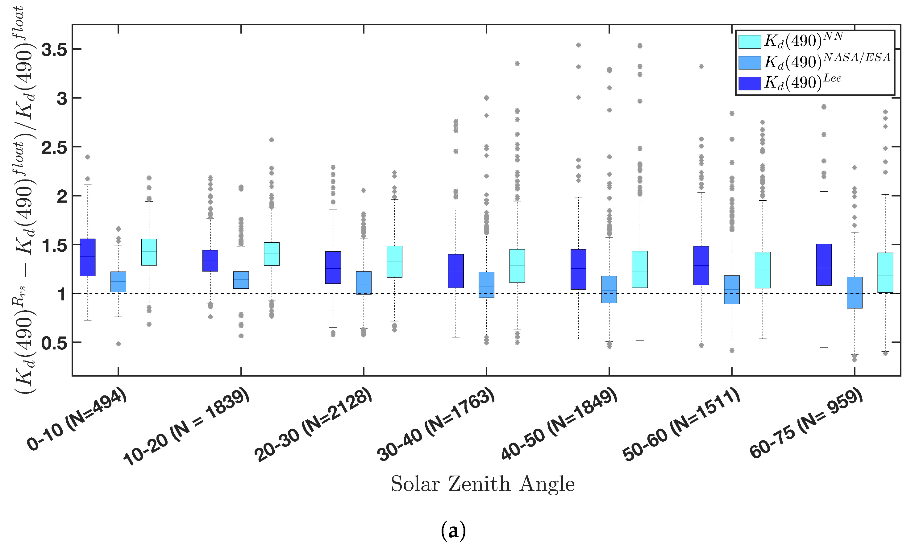
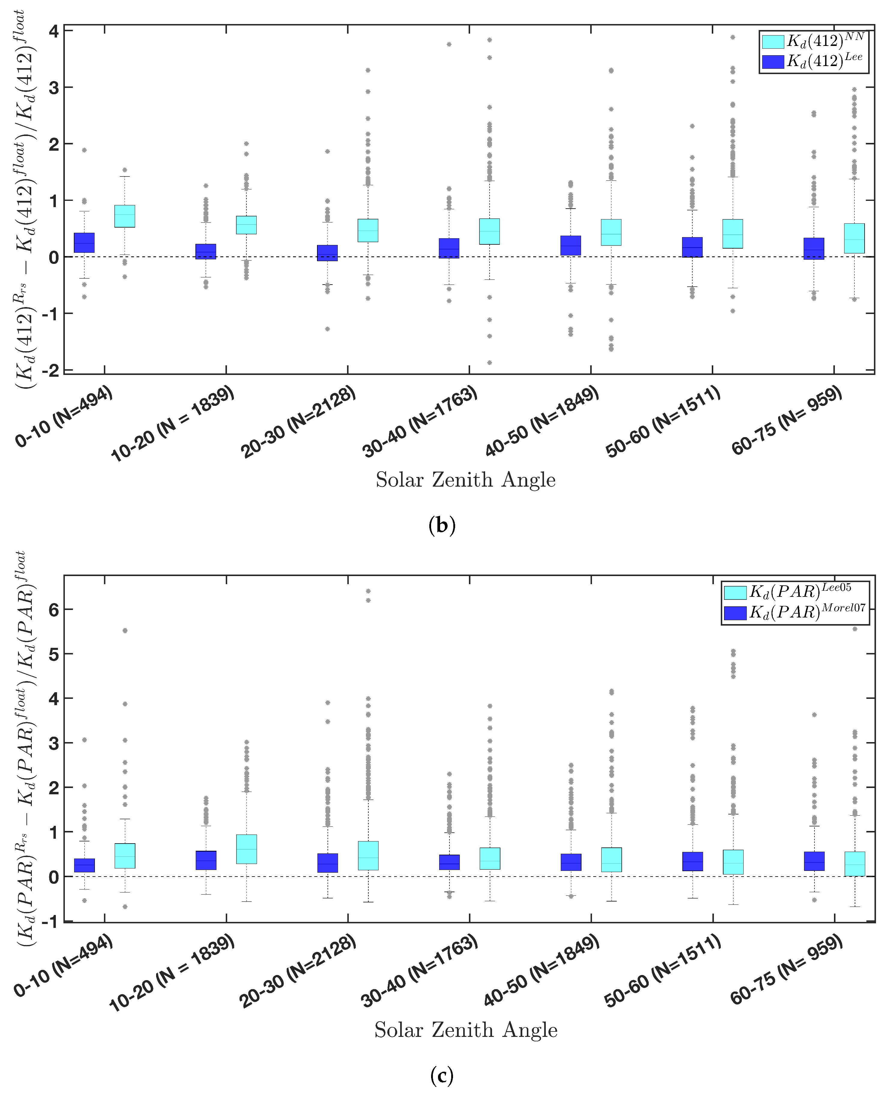
4.3. Influence of the Solar Zenith Angle
5. Conclusions
Author Contributions
Funding
Data Availability Statement
Acknowledgments
Conflicts of Interest
Appendix A. Floats Quality Control and Distribution

| BGC-Argo | Profiles downloaded | 40,738 |
| QC from Organelli et al. | 29,004 | |
| 5 values within the upper 10 m | 25,090 | |
| Satellite | Images downloaded | 364,813 |
| Images passing matchups criteria | 10,873 | |
| Images passing QWIP [16] | 10,805 |
Appendix B. Biomes Separation
| Biome Number | Biome Acronym | Biome Name | Float Proportion (in %) | Oceanic Coverage Proportion (in%) |
|---|---|---|---|---|
| 1 | `NP ICE’ | North Pacific Ice | 0 | 1.37 |
| 2 | `NP SPSS’ | North Pacific Subpolar Seasonally Stratified | 0 | 3.85 |
| 3 | `NP STSS’ | North Pacific Subtropical Seasonally Stratified | 0 | 2.04 |
| 4 | ’NP STPS’ | North Pacific Subtropical Permanently Stratified | 1.21 | 12.29 |
| 5 | `PEQU-W’ | West pacific Equatorial | 0 | 3.50 |
| 6 | `PEQU-E’ | East Pacific Equatorial | 1.36 | 4.46 |
| 7 | `SP STPS’ | South Pacific Subtropical Permanently Stratified | 4.65 | 15.79 |
| 8 | ’NA ICE’ | North Atlantic Ice | 2.67 | 1.64 |
| 9 | `NA SPSS’ | North Atlantic Subpolar Seasonally Stratified | 6.53 | 3.01 |
| 10 | `NA STSS’ | North Atlantic Subtropical Seasonally Stratified | 0.51 | 1.79 |
| 11 | `NA STPS’ | North Atlantic Subtropical Permanently Stratified | 4.69 | 5.23 |
| 12 | `AEQU’ | Atlantic Equatorial | 0.18 | 2.22 |
| 13 | `SA STPS’ | South Atlantic Subtropical Permanently Stratified | 8.88 | 5.41 |
| 14 | `IND STPS’ | Indian Ocean Subtropical Permanently Stratified | 0.17 | 10.76 |
| 15 | `SO STSS’ | Southern Ocean Subtropical Seasonally Stratified | 4.62 | 8.89 |
| 16 | `SO SPSS’ | Southern Ocean Subpolar Seasonally Stratified | 3.49 | 11.87 |
| 17 | `SO ICE’ | Southern Ocean Ice | 0.036 | 5.59 |
| 18 | `W MED’ | Western Mediterranean | 32.75 | 0.22 |
| 19 | `E MED’ | Eastern Mediterranean | 28.25 | 0.56 |
Appendix C. COASTLOOC and NOMAD Comparison
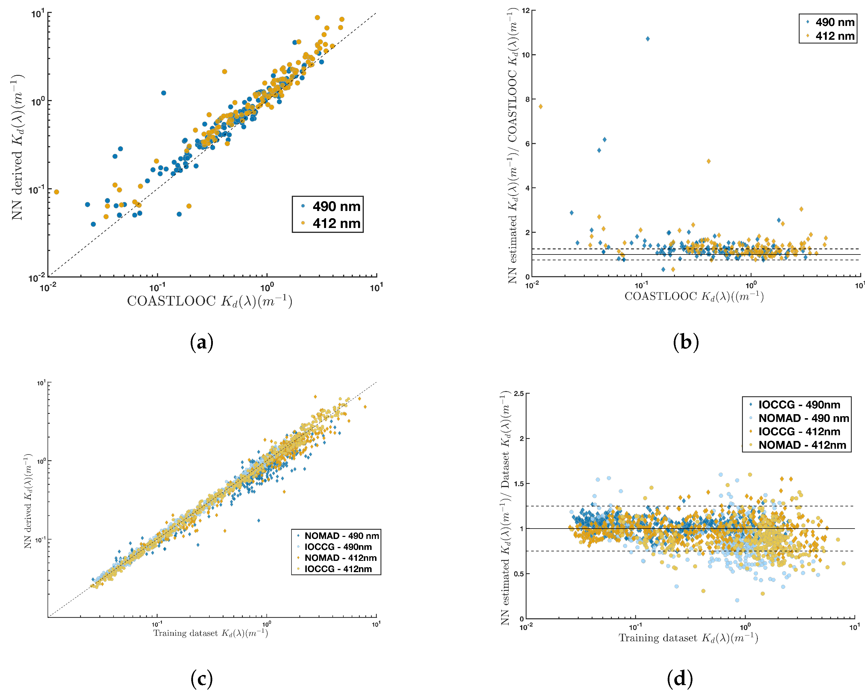
| COASTLOOC | NOMAD | IOCCG | ||||
|---|---|---|---|---|---|---|
| 490 | 412 | 490 | 412 | 490 | 412 | |
| Slope | 1.10 | 1.43 | 0.68 | 0.82 | 1.00 | 1.02 |
| Intercept | 0.060 | −0.132 | 0.103 | 0.095 | −0.002 | −0.019 |
| r | 0.92 | 0.92 | 0.89 | 0.90 | 0.99 | 0.99 |
| RMSD | 0.319 | 0.855 | 0.373 | 0.530 | 0.062 | 0.206 |
Appendix D. Satellite-Floats Retrieval Slopes Forced to 0
| Sensor & Algorithm | BIAS | APD | RMSD | r | Slope |
|---|---|---|---|---|---|
| MODIS-Terra: | 1.19 | 27.14 | 0.018 | 0.87 | 1.11 |
| MODIS-Terra: | 1.24 | 30.76 | 0.020 | 0.84 | 1.16 |
| MODIS-Terra: | 1.08 | 19.97 | 0.018 | 0.86 | 1.04 |
| MODIS-Aqua: | 1.229 | 29.25 | 0.026 | 0.705 | 1.144 |
| MODIS-Aqua: | 1.219 | 29.88 | 0.021 | 0.804 | 1.132 |
| MODIS-Aqua: | 1.081 | 20.08 | 0.019 | 0.830 | 1.049 |
| VIIRS-SNPP: | 1.289 | 34.65 | 0.022 | 0.828 | 1.190 |
| VIIRS-SNPP: | 1.017 | 19.46 | 0.021 | 0.833 | 0.979 |
| VIIRS-JPSS: | 1.272 | 32.91 | 0.021 | 0.836 | 1.174 |
| VIIRS-JPSS: | 1.007 | 18.89 | 0.020 | 0.840 | 0.969 |
| OLCI-S3A: | 1.280 | 30.73 | 0.019 | 0.708 | 1.205 |
| OLCI-S3A: | 1.154 | 25.91 | 0.020 | 0.648 | 1.073 |
| OLCI-S3A: | 1.050 | 18.34 | 0.018 | 0.715 | 1.013 |
| OLCI-S3B: | 1.384 | 39.70 | 0.017 | 0.895 | 1.314 |
| OLCI-S3B: | 1.360 | 40.97 | 0.020 | 0.818 | 1.304 |
| OLCI-S3A: | 1.116 | 19.44 | 0.013 | 0.905 | 1.061 |
Appendix E. Variation in Solar Zenith Angle
| Sensor & Algorithm | BIAS | APD | RMSD | r | Slope | Intercept |
|---|---|---|---|---|---|---|
| MODIS-Terra: | 1.21 | 29.49 | 0.023 | 0.85 | 0.88 | 0.012 |
| MODIS-Terra: | 1.27 | 34.11 | 0.025 | 0.82 | 0.88 | 0.014 |
| MODIS-Terra: | 1.07 | 19.83 | 0.023 | 0.85 | 0.91 | 0.006 |
| MODIS-Aqua: | 1.24 | 32.05 | 0.038 | 0.62 | 0.86 | 0.016 |
| MODIS-Aqua: | 1.24 | 34.04 | 0.028 | 0.79 | 0.75 | 0.020 |
| MODIS-Aqua: | 1.08 | 21.98 | 0.025 | 0.82 | 0.89 | 0.009 |
| VIIRS-SNPP: | 1.30 | 35.65 | 0.027 | 0.84 | 0.84 | 0.018 |
| VIIRS-SNPP: | 1.02 | 19.76 | 0.026 | 0.85 | 0.83 | 0.008 |
| VIIRS-JPS: | 1.28 | 33.79 | 0.026 | 0.85 | 0.92 | 0.013 |
| VIIRS-JPSS: | 1.01 | 18.98 | 0.025 | 0.86 | 0.85 | 0.007 |
| OLCI-S3A: | 1.26 | 28.99 | 0.021 | 0.71 | 0.93 | 0.009 |
| OLCI-S3A: | 1.15 | 25.41 | 0.022 | 0.66 | 0.88 | 0.007 |
| OLCI-S3A: | 1.02 | 18.42 | 0.021 | 0.71 | 0.74 | 0.008 |
| OLCI-S3B: | 1.32 | 34.68 | 0.016 | 0.93 | 0.61 | 0.022 |
| OLCI-S3B: | 1.25 | 32.64 | 0.018 | 0.90 | 0.61 | 0.020 |
| OLCI-S3B: | 1.08 | 17.45 | 0.015 | 0.93 | 0.63 | 0.014 |
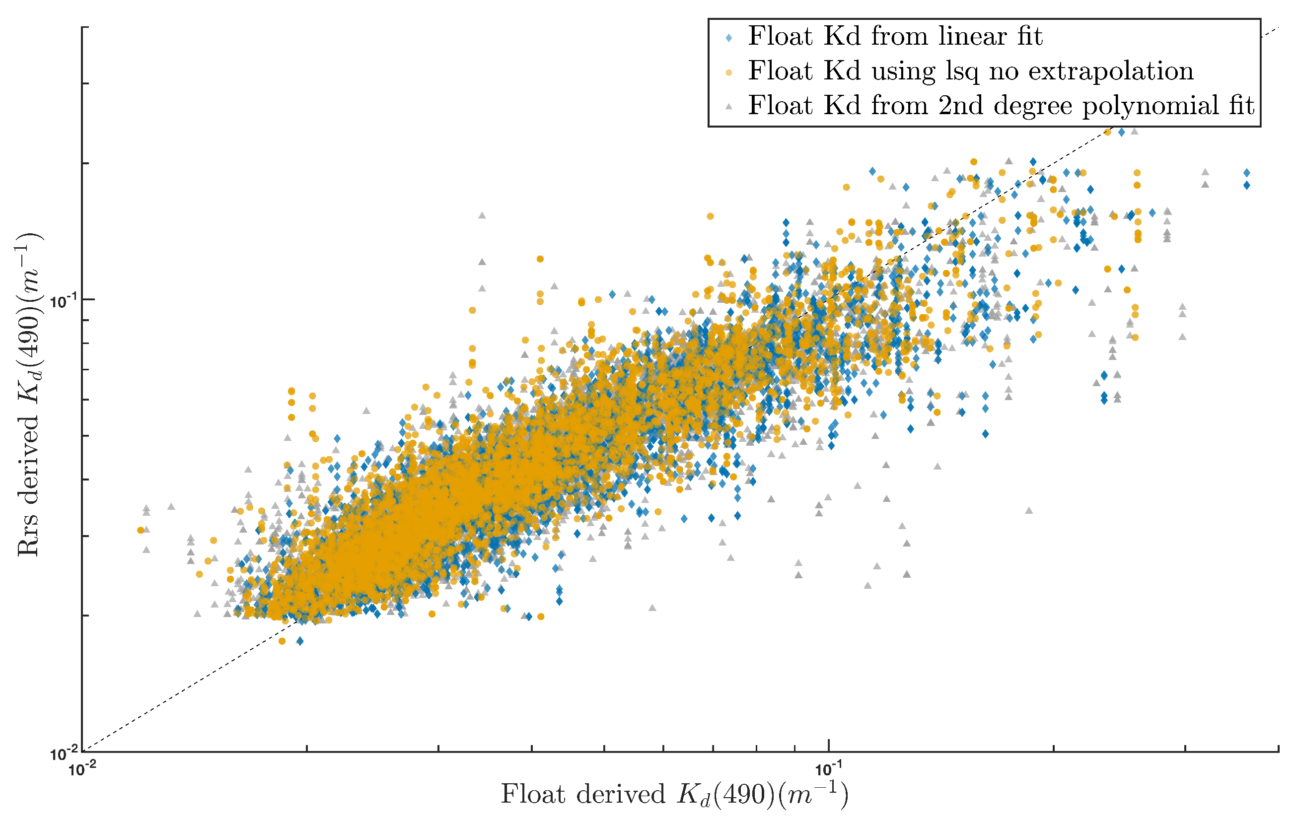
Appendix F. Retrieval Method for Float
Appendix G. Biomes Correlation and Analysis
| MODIS-TERRA | |||||||||||||||||||||||||||||||||
|---|---|---|---|---|---|---|---|---|---|---|---|---|---|---|---|---|---|---|---|---|---|---|---|---|---|---|---|---|---|---|---|---|---|
| Biome 4 | Biome 6 | Biome 7 | Biome 8 | Biome 9 | Biome 11 | Biome 13 | Biome 15 | Biome 16 | Biome 18 | Biome 19 | |||||||||||||||||||||||
| Lee | NN | NASA/ESA | Lee | NN | NASA/ESA | Lee | NN | NASA/ESA | Lee | NN | NASA/ESA | Lee | NN | NASA/ESA | Lee | NN | NASA/ESA | Lee | NN | NASA/ESA | Lee | NN | NASA/ESA | Lee | NN | NASA/ESA | Lee | NN | NASA/ESA | Lee | NN | NASA/ESA | |
| BIAS | 1.14 | 1.27 | 1.07 | 1.27 | 1.26 | 1.25 | 1.45 | 1.50 | 1.13 | 0.99 | 1.13 | 0.91 | 1.02 | 1.00 | 0.95 | 1.27 | 1.31 | 1.00 | 1.40 | 1.49 | 1.07 | 1.16 | 1.15 | 1.12 | 1.32 | 1.35 | 1.14 | 1.11 | 1.12 | 1.05 | 1.21 | 1.25 | 1.07 |
| ADP | 22.15 | 31.17 | 15.84 | 22.61 | 28.31 | 30.18 | 36.78 | 41.05 | 18.28 | 51.63 | 52.92 | 45.05 | 25.64 | 29.51 | 24.12 | 28.41 | 32.04 | 19.49 | 38.76 | 46.87 | 15.80 | 27.76 | 27.33 | 22.25 | 28.97 | 33.40 | 18.51 | 26.61 | 28.05 | 21.95 | 25.18 | 29.51 | 18.59 |
| RMSD | 0.01 | 0.01 | 0.01 | 0.01 | 0.01 | 0.01 | 0.01 | 0.01 | 0.01 | 0.04 | 0.04 | 0.03 | 0.04 | 0.05 | 0.04 | 0.01 | 0.01 | 0.01 | 0.01 | 0.01 | 0.01 | 0.03 | 0.03 | 0.03 | 0.02 | 0.02 | 0.02 | 0.02 | 0.02 | 0.01 | 0.01 | 0.01 | 0.01 |
| r | 0.64 | 0.52 | 0.73 | 0.02 | 0.32 | 0.26 | 0.74 | 0.80 | 0.85 | −0.65 | −0.70 | −0.70 | 0.79 | 0.73 | 0.78 | 0.55 | 0.45 | 0.47 | 0.34 | 0.32 | 0.30 | 0.58 | 0.59 | 0.59 | 0.84 | 0.83 | 0.84 | 0.85 | 0.82 | 0.85 | 0.91 | 0.90 | 0.90 |
| Slope | 0.48 | 0.49 | 0.51 | 1.12 | 1.05 | 1.04 | 0.82 | 0.78 | 1.15 | −0.55 | −0.63 | −0.22 | 0.60 | 0.49 | 0.55 | 0.56 | 0.47 | 0.54 | 0.49 | 0.48 | 0.47 | 0.44 | 0.41 | 0.47 | 1.35 | 1.14 | 1.19 | 0.72 | 0.72 | 0.76 | 0.80 | 0.83 | 0.67 |
| Intercept | 0.02 | 0.02 | 0.02 | 0.00 | 0.01 | 0.01 | 0.01 | 0.01 | 0.00 | 0.12 | 0.13 | 0.09 | 0.03 | 0.04 | 0.03 | 0.02 | 0.02 | 0.01 | 0.02 | 0.02 | 0.01 | 0.04 | 0.04 | 0.03 | −0.01 | 0.01 | 0.00 | 0.02 | 0.02 | 0.01 | 0.01 | 0.01 | 0.01 |
| MODIS-AQUA | |||||||||||||||||||||||||||||||||
| Biome 4 | Biome 6 | Biome 7 | Biome 8 | Biome 9 | Biome 11 | Biome 13 | Biome 15 | Biome 16 | Biome 18 | Biome 19 | |||||||||||||||||||||||
| Lee | NN | NASA/ESA | Lee | NN | NASA/ESA | Lee | NN | NASA/ESA | Lee | NN | NASA/ESA | Lee | NN | NASA/ESA | Lee | NN | NASA/ESA | Lee | NN | NASA/ESA | Lee | NN | NASA/ESA | Lee | NN | NASA/ESA | Lee | NN | NASA/ESA | Lee | NN | NASA/ESA | |
| BIAS | 1.44 | 1.39 | 1.21 | 1.27 | 1.26 | 1.25 | 1.32 | 1.37 | 1.00 | 1.16 | 1.19 | 1.07 | 1.07 | 1.03 | 1.00 | 1.33 | 1.39 | 1.00 | 1.44 | 1.52 | 1.08 | 1.13 | 1.11 | 1.02 | 1.26 | 1.34 | 1.13 | 1.09 | 1.08 | 1.00 | 1.22 | 1.24 | 1.03 |
| ADP | 40.01 | 37.00 | 24.63 | 22.61 | 28.31 | 30.18 | 38.86 | 38.41 | 15.05 | 34.26 | 38.25 | 26.67 | 25.92 | 28.71 | 23.96 | 35.42 | 35.33 | 19.79 | 34.62 | 41.40 | 13.50 | 31.23 | 31.09 | 24.66 | 33.05 | 38.08 | 26.42 | 27.56 | 26.79 | 20.16 | 27.95 | 28.51 | 18.09 |
| RMSD | 0.01 | 0.01 | 0.01 | 0.01 | 0.01 | 0.01 | 0.01 | 0.01 | 0.00 | 0.03 | 0.03 | 0.02 | 0.04 | 0.04 | 0.04 | 0.01 | 0.01 | 0.01 | 0.01 | 0.01 | 0.01 | 0.03 | 0.03 | 0.03 | 0.02 | 0.02 | 0.02 | 0.02 | 0.02 | 0.02 | 0.01 | 0.01 | 0.01 |
| r | −0.56 | −0.46 | −0.29 | 0.02 | 0.32 | 0.26 | 0.92 | 0.90 | 0.94 | −0.10 | −0.15 | −0.05 | 0.75 | 0.70 | 0.74 | 0.64 | 0.68 | 0.69 | 0.84 | 0.81 | 0.87 | 0.51 | 0.47 | 0.53 | 0.80 | 0.79 | 0.76 | 0.81 | 0.79 | 0.82 | 0.87 | 0.87 | 0.84 |
| Slope | −0.72 | −0.75 | −0.45 | 1.12 | 1.05 | 1.04 | 0.89 | 0.72 | 1.12 | −0.93 | −1.00 | −0.77 | 0.56 | 0.45 | 0.58 | 0.68 | 0.64 | 0.75 | 0.77 | 0.76 | 0.87 | 0.47 | 0.43 | 0.51 | 1.14 | 1.02 | 1.04 | 0.84 | 0.78 | 0.88 | 0.85 | 0.79 | 0.73 |
| Intercept | 0.06 | 0.06 | 0.05 | 0.00 | 0.01 | 0.01 | 0.01 | 0.02 | 0.00 | 0.15 | 0.16 | 0.13 | 0.04 | 0.04 | 0.03 | 0.02 | 0.02 | 0.01 | 0.01 | 0.02 | 0.00 | 0.04 | 0.04 | 0.03 | 0.01 | 0.01 | 0.00 | 0.02 | 0.02 | 0.01 | 0.01 | 0.02 | 0.01 |
| VIIRS SNPP | |||||||||||||||||||||||||||||||||
| Biome 4 | Biome 6 | Biome 7 | Biome 8 | Biome 9 | Biome 11 | Biome 13 | Biome 15 | Biome 16 | Biome 18 | Biome 19 | |||||||||||||||||||||||
| Lee | NN | NASA/ESA | Lee | NN | NASA/ESA | Lee | NN | NASA/ESA | Lee | NN | NASA/ESA | Lee | NN | NASA/ESA | Lee | NN | NASA/ESA | Lee | NN | NASA/ESA | Lee | NN | NASA/ESA | Lee | NN | NASA/ESA | Lee | NN | NASA/ESA | Lee | NN | NASA/ESA | |
| BIAS | 1.34 | NaN | 1.07 | 1.33 | NaN | 1.11 | 1.37 | NaN | 0.97 | 1.12 | NaN | 0.94 | 1.05 | NaN | 0.91 | 1.41 | NaN | 1.00 | 1.47 | 1.01 | 1.23 | NaN | 1.03 | 1.31 | NaN | 1.02 | 1.17 | NaN | 0.95 | 1.36 | NaN | 1.03 | |
| ADP | 36.85 | NaN | 11.91 | 38.28 | NaN | 22.57 | 45.05 | NaN | 14.01 | 30.78 | NaN | 33.20 | 28.43 | NaN | 25.23 | 41.28 | NaN | 14.28 | 42.20 | 14.48 | 33.26 | NaN | 20.21 | 40.02 | NaN | 22.51 | 31.46 | NaN | 20.01 | 36.50 | NaN | 18.68 | |
| RMSD | 0.01 | NaN | 0.00 | 0.01 | NaN | 0.01 | 0.01 | NaN | 0.00 | 0.03 | NaN | 0.03 | 0.04 | NaN | 0.04 | 0.01 | NaN | 0.00 | 0.01 | 0.01 | 0.02 | NaN | 0.02 | 0.02 | NaN | 0.02 | 0.02 | NaN | 0.02 | 0.02 | NaN | 0.02 | |
| r | 0.63 | NaN | 0.73 | 0.64 | NaN | 0.49 | 0.84 | NaN | 0.86 | −0.08 | NaN | −0.12 | 0.73 | NaN | 0.74 | 0.67 | NaN | 0.69 | 0.78 | 0.80 | 0.58 | NaN | 0.59 | 0.57 | NaN | 0.53 | 0.77 | NaN | 0.77 | 0.81 | NaN | 0.80 | |
| Slope | 0.81 | NaN | 0.79 | 0.29 | NaN | 0.39 | 0.92 | NaN | 0.96 | −0.48 | NaN | −0.40 | 0.61 | NaN | 0.58 | 0.68 | NaN | 0.60 | 0.87 | 0.87 | 0.53 | NaN | 0.52 | 0.74 | NaN | 0.65 | 0.74 | NaN | 0.73 | 0.66 | NaN | 0.56 | |
| Intercept | 0.02 | NaN | 0.01 | 0.04 | NaN | 0.03 | 0.01 | NaN | 0.00 | 0.11 | NaN | 0.09 | 0.04 | NaN | 0.03 | 0.02 | NaN | 0.01 | 0.01 | 0.00 | 0.04 | NaN | 0.03 | 0.02 | NaN | 0.02 | 0.02 | NaN | 0.01 | 0.02 | NaN | 0.01 | |
| VIIRS JPSS | |||||||||||||||||||||||||||||||||
| Biome 4 | Biome 6 | Biome 7 | Biome 8 | Biome 9 | Biome 11 | Biome 13 | Biome 15 | Biome 16 | Biome 18 | Biome 19 | |||||||||||||||||||||||
| Lee | NN | NASA/ESA | Lee | NN | NASA/ESA | Lee | NN | NASA/ESA | Lee | NN | NASA/ESA | Lee | NN | NASA/ESA | Lee | NN | NASA/ESA | Lee | NN | NASA/ESA | Lee | NN | NASA/ESA | Lee | NN | NASA/ESA | Lee | NN | NASA/ESA | Lee | NN | NASA/ESA | |
| BIAS | 1.36 | NaN | 1.06 | 1.34 | NaN | 1.12 | 1.28 | NaN | 0.94 | 0.99 | NaN | 0.85 | 1.07 | NaN | 0.90 | 1.38 | NaN | 0.98 | 1.39 | NaN | 0.96 | 1.23 | NaN | 1.02 | 1.23 | NaN | 0.94 | 1.14 | NaN | 0.93 | 1.33 | NaN | 1.02 |
| ADP | 32.62 | NaN | 10.48 | 36.67 | NaN | 16.84 | 38.38 | NaN | 11.95 | 22.87 | NaN | 29.39 | 26.94 | NaN | 24.07 | 40.59 | NaN | 15.13 | 39.60 | NaN | 14.95 | 33.88 | NaN | 22.69 | 36.31 | NaN | 19.07 | 30.09 | NaN | 19.25 | 34.61 | NaN | 18.16 |
| RMSD | 0.01 | NaN | 0.00 | 0.01 | NaN | 0.01 | 0.01 | NaN | 0.00 | 0.02 | NaN | 0.03 | 0.04 | NaN | 0.04 | 0.01 | NaN | 0.01 | 0.01 | NaN | 0.01 | 0.03 | NaN | 0.03 | 0.02 | NaN | 0.01 | 0.02 | NaN | 0.02 | 0.02 | NaN | 0.02 |
| r | 0.53 | NaN | 0.66 | 0.59 | NaN | 0.57 | 0.83 | NaN | 0.85 | −0.05 | NaN | −0.07 | 0.75 | NaN | 0.76 | 0.23 | NaN | 0.23 | 0.80 | NaN | 0.83 | 0.51 | NaN | 0.52 | 0.88 | NaN | 0.84 | 0.79 | NaN | 0.78 | 0.80 | NaN | 0.80 |
| Slope | 0.68 | NaN | 0.65 | 0.86 | NaN | 1.04 | 0.89 | NaN | 0.94 | −0.56 | NaN | −0.47 | 0.67 | NaN | 0.61 | 0.57 | NaN | 0.47 | 0.76 | NaN | 0.75 | 0.47 | NaN | 0.47 | 0.98 | NaN | 0.86 | 0.77 | NaN | 0.76 | 0.67 | NaN | 0.56 |
| Intercept | 0.02 | NaN | 0.01 | 0.02 | NaN | 0.00 | 0.01 | NaN | 0.00 | 0.12 | NaN | 0.10 | 0.03 | NaN | 0.03 | 0.02 | NaN | 0.01 | 0.01 | NaN | 0.01 | 0.04 | NaN | 0.03 | 0.01 | NaN | 0.01 | 0.02 | NaN | 0.01 | 0.02 | NaN | 0.01 |
| OLCI-S3A | |||||||||||||||||||||||||||||||||
| Biome 4 | Biome 6 | Biome 7 | Biome 8 | Biome 9 | Biome 11 | Biome 13 | Biome 15 | Biome 16 | Biome 18 | Biome 19 | |||||||||||||||||||||||
| Lee | NN | NASA/ESA | Lee | NN | NASA/ESA | Lee | NN | NASA/ESA | Lee | NN | NASA/ESA | Lee | NN | NASA/ESA | Lee | NN | NASA/ESA | Lee | NN | NASA/ESA | Lee | NN | NASA/ESA | Lee | NN | NASA/ESA | Lee | NN | NASA/ESA | Lee | NN | NASA/ESA | |
| BIAS | 1.31 | 1.17 | 1.05 | 1.25 | 1.22 | 1.04 | 1.21 | 1.07 | 0.96 | 0.83 | 0.78 | 0.74 | 1.01 | 1.00 | 0.89 | 1.34 | 1.15 | 1.04 | 1.40 | 1.26 | 1.08 | 1.23 | 1.24 | 1.02 | 1.23 | 1.24 | 0.94 | 1.04 | 0.92 | 0.85 | 1.23 | 1.05 | 0.99 |
| ADP | 26.90 | 22.85 | 17.54 | 43.62 | 44.44 | 25.28 | 24.28 | 23.40 | 17.45 | 52.60 | 78.07 | 74.93 | 12.40 | 14.11 | 15.95 | 29.48 | 21.40 | 14.75 | 32.93 | 26.03 | 12.64 | 33.88 | 28.51 | 22.69 | 36.31 | 28.51 | 19.07 | 32.75 | 32.76 | 20.51 | 32.88 | 25.26 | 17.77 |
| RMSD | 0.01 | 0.01 | 0.01 | 0.02 | 0.02 | 0.01 | 0.01 | 0.01 | 0.01 | 0.04 | 0.05 | 0.05 | 0.01 | 0.01 | 0.01 | 0.01 | 0.01 | 0.00 | 0.01 | 0.01 | 0.00 | 0.03 | 0.01 | 0.03 | 0.02 | 0.01 | 0.01 | 0.02 | 0.02 | 0.01 | 0.02 | 0.02 | 0.01 |
| r | 0.52 | 0.53 | 0.56 | 0.94 | 0.97 | 0.96 | 0.67 | 0.58 | 0.64 | NAN | NaN | NaN | 0.93 | 0.90 | 0.93 | 0.65 | 0.61 | 0.78 | 0.19 | −0.03 | 0.19 | 0.51 | 0.87 | 0.52 | 0.88 | 0.87 | 0.84 | 0.85 | 0.68 | 0.89 | 0.65 | 0.58 | 0.64 |
| Slope | 0.64 | 0.74 | 0.57 | 1.41 | 2.36 | 1.41 | 0.95 | 0.97 | 0.81 | NAN | NaN | NaN | 1.06 | 0.92 | 1.09 | 1.02 | 1.08 | 0.84 | 1.56 | −1.57 | 0.99 | 0.47 | 0.79 | 0.47 | 0.98 | 0.79 | 0.86 | 0.62 | 0.83 | 0.63 | 0.71 | 0.84 | 0.67 |
| Intercept | 0.02 | 0.01 | 0.01 | 0.00 | -0.03 | −0.01 | 0.01 | 0.00 | 0.00 | NAN | NaN | NaN | 0.00 | 0.01 | −0.01 | 0.01 | 0.00 | 0.00 | −0.01 | 0.06 | 0.00 | 0.04 | 0.02 | 0.03 | 0.01 | 0.02 | 0.01 | 0.02 | 0.01 | 0.02 | 0.02 | 0.01 | 0.01 |
| OLCI-S3B | |||||||||||||||||||||||||||||||||
| Biome 4 | Biome 6 | Biome 7 | Biome 8 | Biome 9 | Biome 11 | Biome 13 | Biome 15 | Biome 16 | Biome 18 | Biome 19 | |||||||||||||||||||||||
| Lee | NN | NASA/ESA | Lee | NN | NASA/ESA | Lee | NN | NASA/ESA | Lee | NN | NASA/ESA | Lee | NN | NASA/ESA | Lee | NN | NASA/ESA | Lee | NN | NASA/ESA | Lee | NN | NASA/ESA | Lee | NN | NASA/ESA | Lee | NN | NASA/ESA | Lee | NN | NASA/ESA | |
| BIAS | 1.19 | 1.24 | 1.08 | 1.23 | 1.22 | 1.08 | 1.29 | 0.48 | 1.02 | 1.27 | 0.49 | 1.01 | 1.28 | 1.15 | 1.05 | 1.38 | 1.36 | 1.12 | 1.44 | 1.28 | 1.12 | 1.31 | 1.35 | 1.08 | 1.45 | 1.34 | 1.15 | 0.79 | 0.79 | 0.69 | 1.31 | 1.41 | 1.25 |
| ADP | 27.14 | 30.76 | 19.97 | 29.13 | 30.00 | 20.19 | 34.71 | 158.21 | 19.46 | 32.89 | 140.55 | 18.76 | 30.73 | 25.91 | 18.34 | 39.70 | 40.97 | 19.44 | 38.86 | 33.61 | 17.74 | 30.59 | 36.75 | 14.38 | 32.17 | 27.25 | 14.13 | 58.61 | 56.02 | 71.42 | 12.90 | 23.58 | 11.17 |
| RMSD | 0.02 | 0.02 | 0.02 | 0.02 | 0.02 | 0.02 | 0.02 | 0.03 | 0.02 | 0.02 | 0.03 | 0.02 | 0.02 | 0.02 | 0.02 | 0.02 | 0.02 | 0.01 | 0.01 | 0.01 | 0.01 | 0.01 | 0.01 | 0.00 | 0.01 | 0.01 | 0.01 | 0.04 | 0.04 | 0.05 | 0.01 | 0.02 | 0.01 |
| r | 0.87 | 0.84 | 0.86 | 0.83 | 0.81 | 0.83 | 0.82 | 0.73 | 0.82 | NaN | NaN | NaN | 0.71 | 0.65 | 0.71 | 0.90 | 0.82 | 0.91 | 0.70 | 0.46 | 0.87 | 1.00 | 1.00 | 1.00 | 0.97 | 0.97 | 0.97 | 0.79 | 1.00 | 1.00 | 0.96 | 0.81 | 0.96 |
| Slope | 0.79 | 0.78 | 0.80 | 0.83 | 0.75 | 0.86 | 0.79 | 0.91 | 0.76 | NaN | NaN | NaN | 0.92 | 0.83 | 0.72 | 0.87 | 0.67 | 0.63 | 0.55 | 0.51 | 0.52 | 0.10 | 1.40 | 0.00 | 0.82 | 1.08 | 0.79 | 0.08 | 0.07 | 0.07 | 0.94 | 0.78 | 1.01 |
| Intercept | 0.01 | 0.02 | 0.01 | 0.02 | 0.02 | 0.01 | 0.02 | −0.01 | 0.01 | NaN | NaN | NaN | 0.01 | 0.01 | 0.01 | 0.02 | 0.02 | 0.02 | 0.03 | 0.02 | 0.02 | 0.04 | 0.00 | 0.04 | 0.02 | 0.01 | 0.01 | 0.06 | 0.06 | 0.05 | 0.01 | 0.03 | 0.00 |
References
- Mobley, C. The Oceanic Optics Book; International Ocean Colour Coordinating Group (IOCCG): Monterey, CA, USA, 2022. [Google Scholar] [CrossRef]
- Xing, X.; Boss, E.; Zhang, J.; Chai, F. Evaluation of Ocean Color Remote Sensing Algorithms for Diffuse Attenuation Coefficients and Optical Depths with Data Collected on BGC-Argo Floats. Remote Sens. 2020, 12, 2367. [Google Scholar] [CrossRef]
- Jamet, C.; Loisel, H.; Dessailly, D. Retrieval of the spectral diffuse attenuation coefficient Kd(λ) in open and coastal ocean waters using a neural network inversion: Retrieval of Diffuse Attenuation. J. Geophys. Res. Ocean. 2012, 117, C10023. [Google Scholar] [CrossRef]
- Morel, A.; Huot, Y.; Gentili, B.; Werdell, P.J.; Hooker, S.B.; Franz, B.A. Examining the consistency of products derived from various ocean color sensors in open ocean (Case 1) waters in the perspective of a multi-sensor approach. Remote Sens. Environ. 2007, 111, 69–88. [Google Scholar] [CrossRef]
- Incorporated, S. OCR 504 User Manual; Technical Report. Available online: https://www.seabird.com/asset-get.download.jsa?id=54627868876 (accessed on 21 July 2022).
- Organelli, E.; Claustre, H.; Bricaud, A.; Barbieux, M.; Uitz, J.; D’Ortenzio, F.; Dall’Olmo, G. Bio-optical anomalies in the world’s oceans: An investigation on the diffuse attenuation coefficients for downward irradiance derived from Biogeochemical Argo float measurements: WORLD’S OCEAN BIO-OPTICAL ANOMALIES. J. Geophys. Res. Ocean. 2017, 122, 3543–3564. [Google Scholar] [CrossRef]
- Gordon, H.R.; McCluney, W.R. Estimation of the Depth of Sunlight Penetration in the Sea for Remote Sensing. Appl. Opt. 1975, 14, 413. [Google Scholar] [CrossRef] [PubMed]
- Mueller, J. SeaWiFS Algorithm for the Diffuse Attenuation Coefficient, K(490), Using Water-Leaving Radiances at 490 and 555 nm; Technical Report Part 3; NASA Goddard Space Flight Center: Greenbelt, MD, USA, 2000. [Google Scholar]
- Morel, A. Optical modeling of the upper ocean in relation to its biogenous matter content (case I waters). J. Geophys. Res. Ocean. 1988, 93, 10749–10768. [Google Scholar] [CrossRef]
- Werdell, P.J.; Bailey, S.W. An improved in-situ bio-optical dataset for ocean color algorithm development and satellite data product validation. Remote Sens. Environ. 2005, 98, 122–140. [Google Scholar] [CrossRef]
- IOCCG. Remote Sensing of Inherent Optical Properties: Fundamentals, Tests of Algorithms, and Applications; Technical Report 5; IOCCG: Dartmouth, NS, Canada, 2006. [Google Scholar]
- Fay, A.R.; McKinley, G.A. Global open-ocean biomes: Mean and temporal variability. Earth Syst. Sci. Data 2014, 6, 273–284. [Google Scholar] [CrossRef]
- Bailey, S.W.; Werdell, P.J. A multi-sensor approach for the on-orbit validation of ocean color satellite data products. Remote Sens. Environ. 2006, 102, 12–23. [Google Scholar] [CrossRef]
- Bisson, K.M.; Boss, E.; Westberry, T.K.; Behrenfeld, M.J. Evaluating satellite estimates of particulate backscatter in the global open ocean using autonomous profiling floats. Opt. Express 2019, 27, 30191. [Google Scholar] [CrossRef]
- Zhang, T.; Fell, F. An empirical algorithm for determining the diffuse attenuation coefficient Kd in clear and turbid waters from spectral remote sensing reflectance: Kd in clear and turbid waters. Limnol. Oceanogr. Methods 2007, 5, 457–462. [Google Scholar] [CrossRef]
- Dierssen, H.M.; Vandermeulen, R.A.; Barnes, B.B.; Castagna, A.; Knaeps, E.; Vanhellemont, Q. QWIP: A Quantitative Metric for Quality Control of Aquatic Reflectance Spectral Shape Using the Apparent Visible Wavelength. Front. Remote. Sens. 2022, 3, 869611. [Google Scholar] [CrossRef]
- Austin, R.W.; Petzold, T.J. The Determination of the Diffuse Attenuation Coefficient of Sea Water Using the Coastal Zone Color Scanner. In Oceanography from Space; Gower, J.F.R., Ed.; Springer: Boston, MA, USA, 1981; pp. 239–256. [Google Scholar] [CrossRef]
- Lee, Z.P. Diffuse attenuation coefficient of downwelling irradiance: An evaluation of remote sensing methods. J. Geophys. Res. 2005, 110, C02017. [Google Scholar] [CrossRef]
- Lee, Z.; Carder, K.L.; Arnone, R.A. Deriving inherent optical properties from water color: A multiband quasi-analytical algorithm for optically deep waters. Appl. Opt. 2002, 41, 5755. [Google Scholar] [CrossRef]
- Lee, Z.; Hu, C.; Shang, S.; Du, K.; Lewis, M.; Arnone, R.; Brewin, R. Penetration of UV-visible solar radiation in the global oceans: Insights from ocean color remote sensing: Penetration of UV-Visible Solar Light. J. Geophys. Res. Ocean. 2013, 118, 4241–4255. [Google Scholar] [CrossRef]
- Westberry, T.K.; Boss, E.; Lee, Z. Influence of Raman scattering on ocean color inversion models. Appl. Opt. 2013, 52, 5552. [Google Scholar] [CrossRef]
- Loisel, H.; Stramski, D.; Dessailly, D.; Jamet, C.; Li, L.; Reynolds, R.A. An Inverse Model for Estimating the Optical Absorption and Backscattering Coefficients of Seawater From Remote-Sensing Reflectance Over a Broad Range of Oceanic and Coastal Marine Environments: Inversion of Seawater IOPS. J. Geophys. Res. Ocean. 2018, 123, 2141–2171. [Google Scholar] [CrossRef]
- Xing, X.; Boss, E. Chlorophyll-Based Model to Estimate Underwater Photosynthetically Available Radiation for Modeling, In-Situ, and Remote-Sensing Applications. Geophys. Res. Lett. 2021, 48, e2020GL092189. [Google Scholar] [CrossRef]
- Lee, Z. Penetration of solar radiation in the upper ocean: A numerical model for oceanic and coastal waters. J. Geophys. Res. 2005, 110, C09019. [Google Scholar] [CrossRef]
- Brewin, R.J.; Sathyendranath, S.; Müller, D.; Brockmann, C.; Deschamps, P.Y.; Devred, E.; Doerffer, R.; Fomferra, N.; Franz, B.; Grant, a.; et al. The Ocean Colour Climate Change Initiative: III. A round-robin comparison on in-water bio-optical algorithms. Remote Sens. Environ. 2015, 162, 271–294. [Google Scholar] [CrossRef]
- Yu, X.; Salama, M.S.; Shen, F.; Verhoef, W. Retrieval of the diffuse attenuation coefficient from GOCI images using the 2SeaColor model: A case study in the Yangtze Estuary. Remote Sens. Environ. 2016, 175, 109–119. [Google Scholar] [CrossRef]
- Zhang, Y.; Xu, Z.; Yang, Y.; Wang, G.; Zhou, W.; Cao, W.; Li, Y.; Zheng, W.; Deng, L.; Zeng, K.; et al. Diurnal Variation of the Diffuse Attenuation Coefficient for Downwelling Irradiance at 490 nm in Coastal East China Sea. Remote Sens. 2021, 13, 1676. [Google Scholar] [CrossRef]
- Zheng, X.; Dickey, T.; Chang, G. Variability of the downwelling diffuse attenuation coefficient with consideration of inelastic scattering. Appl. Opt. 2002, 41, 6477. [Google Scholar] [CrossRef] [PubMed]
- Organelli, E.; Leymarie, E.; Zielinski, O.; Uitz, J.; D’Ortenzio, F.; Hervé, C. Hyperspectral Radiometry on Biogeochemical-Argo Floats: A Bright Perspective for Phytoplankton Diversity. Oceanography 2021, 34, 90–91. [Google Scholar] [CrossRef]
- Babin, M. Variations in the light absorption coefficients of phytoplankton, nonalgal particles, and dissolved organic matter in coastal waters around Europe. J. Geophys. Res. 2003, 108, 3211. [Google Scholar] [CrossRef]

| Symbol | Definition |
|---|---|
| APD | Absolute Percentage Difference |
| Absorption | |
| Backscattering | |
| Chlorophyll a concentration | |
| Downwelling irradiance | |
| Downwelling irradiance below the surface | |
| Simulated downwelling irradiance with spectral response function | |
| Relative contribution of molecular scattering to total scattering | |
| Instantaneous Downwelling Photosynthetically Available Radiation | |
| Diffuse attenuation coefficient at 490 nm due to material co-varying with chlorophyll | |
| ESA L2 operational algorithm based on Morel | |
| (,) | Centroid pair, average of and |
| -retrieved | |
| The layer averaged diffuse attenuation coefficient | |
| The layer averaged diffuse attenuation coefficient from the surface to the penetration depth | |
| Lee’s semi-analytical algorithm | |
| Lee’s semi-analytical algorithm retrieving PAR | |
| Morel’s empirical algorithm retrieving PAR | |
| NASA L2 operational algorithm based on Austin& Werdell | |
| Jamet’s neural network algorithm | |
| -retrieved | |
| -retrieved | |
| Diffuse attenuation coefficient at 490 nm of pure water | |
| Simulated water leaving radiance corrected for the spectral response function | |
| Water leaving radiance | |
| Downwelling Photosynthetically Available Radiation | |
| Irradiance reflectance below the surface | |
| Remote Sensing Reflectance | |
| Satellite Remote sensing reflectance | |
| Water leaving reflectance ratio of 490/560 | |
| Sun zenith angle over the surface of the ocean | |
| ,, | Constants for computation of |
| Penetration depth |
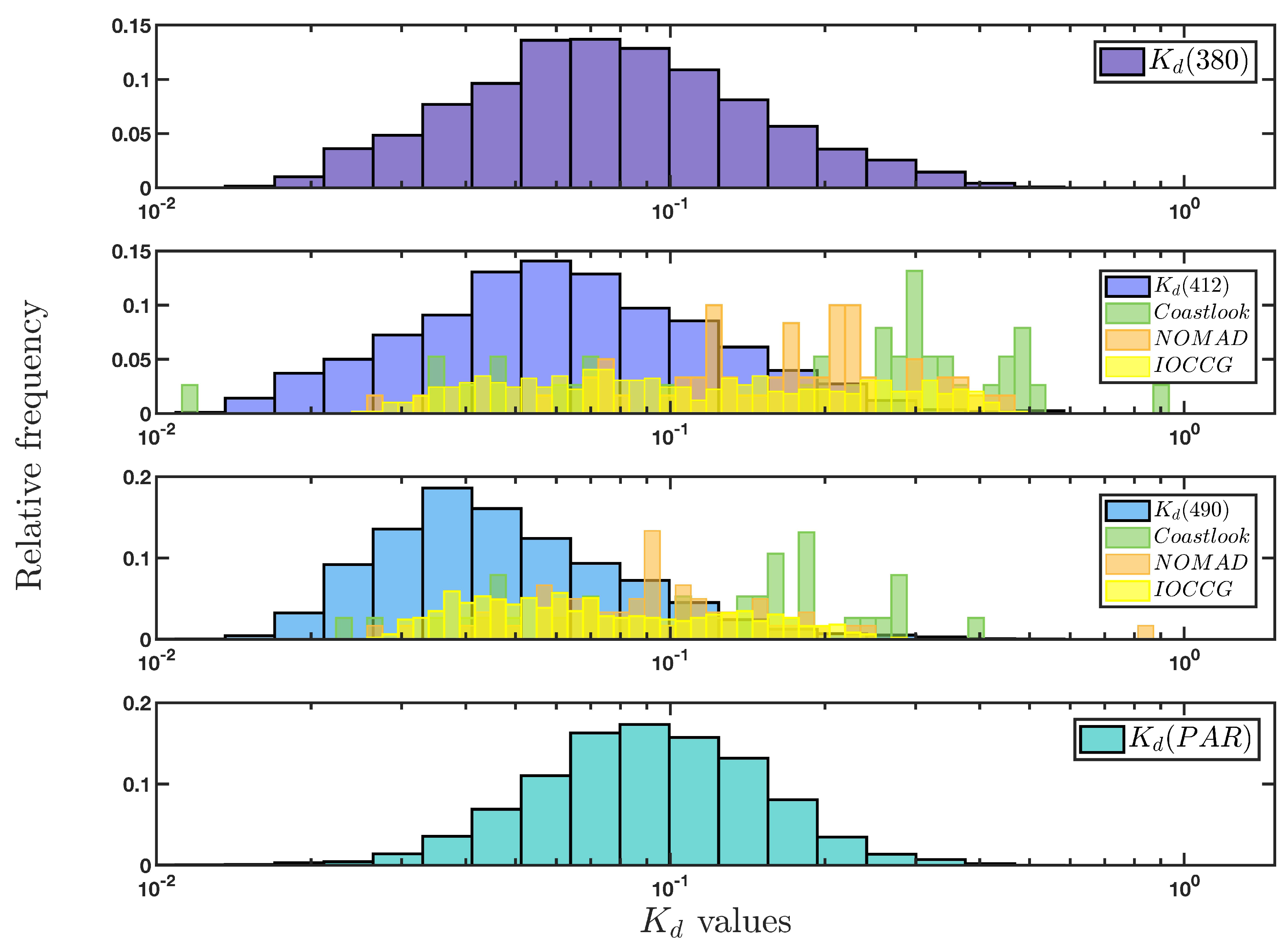
| Wavelengths () | N |
|---|---|
| 380 nm | 22,167 |
| 412 nm | 19,813 |
| 490 nm | 14,876 |
| PAR | 12,552 |
| Total unique float profiles | 29,004 |
| Sensor & Algo | BIAS | APD (%) | RMSD (m−1) | r | Slope | Intercept | N |
|---|---|---|---|---|---|---|---|
| MODIS-Terra: KdLee05 | 1.08 | 18.62 | 0.01 | 0.90 | 0.78 | 0.010 | |
| MODIS-Terra: KdNN | 1.31 | 33.72 | 0.02 | 0.87 | 0.76 | 0.018 | 2144 |
| MODIS-Terra: KdNASA | 1.13 | 20.37 | 0.01 | 0.90 | 0.84 | 0.010 | |
| MODIS-Aqua: KdLee05 | 1.11 | 19.58 | 0.01 | 0.89 | 0.82 | 0.011 | |
| MODIS-Aqua: KdNN | 1.27 | 31.19 | 0.02 | 0.86 | 0.79 | 0.017 | 1802 |
| MODIS-Aqua: KdNASA | 1.12 | 19.67 | 0.01 | 0.89 | 0.89 | 0.009 | |
| VIIRS-SNPP: KdLee05 | 1.16 | 22.46 | 0.02 | 0.88 | 0.77 | 0.013 | 3290 |
| VIIRS-SNPP: KdNASA | 1.06 | 17.36 | 0.02 | 0.88 | 0.78 | 0.010 | |
| VIIRS-SNPP: KdLee05 | 1.16 | 22.46 | 0.02 | 0.88 | 0.77 | 0.013 | 2445 |
| VIIRS-SNPP: KdNASA | 1.06 | 17.36 | 0.02 | 0.88 | 0.78 | 0.010 | |
| OLCI-S3A: KdLee05 | 1.16 | 21.46 | 0.01 | 0.84 | 0.79 | 0.012 | 651 |
| OLCI-S3A: KdNN | 1.19 | 26.62 | 0.01 | 0.77 | 0.91 | 0.008 | |
| OLCI-S3A: KdESA | 1.08 | 17.85 | 0.01 | 0.83 | 0.82 | 0.008 | |
| OLCI-S3B: KdLee05 | 1.25 | 27.73 | 0.01 | 0.91 | 0.68 | 0.018 | |
| OLCI-S3B: KdNN | 1.42 | 43.24 | 0.02 | 0.85 | 0.84 | 0.019 | 382 |
| OLCI-S3B: KdESA | 1.18 | 20.88 | 0.01 | 0.92 | 0.71 | 0.013 |
| Sensor & Algo | BIAS | APD (%) | RMSD | r | Slope | Intercept | N |
|---|---|---|---|---|---|---|---|
| MODIS-Terra: KdLee05 | 1.13 | 11.60 | 0.06 | 0.68 | 0.91 | 0.010 | 1633 |
| MODIS-Terra: KdNN | 1.19 | 19.49 | 0.03 | 0.87 | 1.01 | 0.018 | |
| MODIS-Aqua: KdLee05 | 1.10 | 8.91 | 0.02 | 0.86 | 0.88 | 0.011 | 1384 |
| MODIS-Aqua: KdNN | 1.15 | 16.01 | 0.03 | 0.88 | 1.09 | 0.017 | |
| OLCI-S3A: KdLee05 | 1.19 | 20.68 | 0.02 | 0.93 | 0.98 | 0.012 | 269 |
| OLCI-S3A: KdNN | 1.15 | 13.67 | 0.02 | 0.88 | 0.92 | 0.008 | |
| OLCI-S3B: KdLee05 | 1.23 | 23.23 | 0.02 | 0.92 | 0.85 | 0.018 | 326 |
| OLCI -S3B: KdNN | 1.34 | 35.02 | 0.02 | 0.87 | 1.20 | 0.019 |
| MODIS-Terra | MODIS-Aqua | VIIRS-SNPP | VIIRS-JPSS | OLCI-S3A | OLCI-S3B | |||||||
|---|---|---|---|---|---|---|---|---|---|---|---|---|
| Lee05 | Morel07 | Lee05 | Morel07 | Lee05 | Morel07 | Lee05 | Morel07 | Lee05 | Morel07 | Lee05 | Morel07 | |
| Bias | 1.24 | 1.20 | 1.28 | 1.23 | 1.28 | 1.26 | 1.28 | 1.24 | 1.21 | 1.17 | 1.25 | 1.28 |
| ADP | 23.88 | 21.05 | 28.72 | 26.34 | 30.89 | 29.81 | 28.74 | 28.07 | 20.77 | 15.97 | 33.73 | 33.31 |
| RMSD | 0.027 | 0.032 | 0.031 | 0.035 | 0.031 | 0.037 | 0.029 | 0.035 | 0.028 | 0.034 | 0.026 | 0.028 |
| r | 0.87 | 0.75 | 0.86 | 0.76 | 0.86 | 0.75 | 0.88 | 0.77 | 0.81 | 0.65 | 0.92 | 0.85 |
| Slope | 0.83 | 0.61 | 0.90 | 0.68 | 0.82 | 0.57 | 0.77 | 0.53 | 0.85 | 0.53 | 0.94 | 0.69 |
| Intercept | 0.029 | 0.044 | 0.028 | 0.044 | 0.035 | 0.053 | 0.036 | 0.053 | 0.024 | 0.045 | 0.025 | 0.042 |
| Biome 4 (N = 113) | Biome 6 (N = 35) | Biome 7 (N = 239) | Biome 8 (N = 76) | Biome 9 (N = 435) | |||||||||||
|---|---|---|---|---|---|---|---|---|---|---|---|---|---|---|---|
| Lee | Jamet | Austin | Lee | Jamet | Austin | Lee | Jamet | Austin | Lee | Jamet | Austin | Lee | Jamet | Austin | |
| BIAS | 1.13 | 1.25 | 1.08 | 1.16 | 1.35 | 1.20 | 1.18 | 1.31 | 1.11 | 0.95 | 1.04 | 0.88 | 0.97 | 1.01 | 0.96 |
| ADP | 17.57 | 29.58 | 13.65 | 18.38 | 35.04 | 21.08 | 19.92 | 35.38 | 14.38 | 25.38 | 30.85 | 25.90 | 21.03 | 25.30 | 20.72 |
| RMSD | 0.01 | 0.01 | 0.01 | 0.01 | 0.02 | 0.01 | 0.01 | 0.01 | 0.01 | 0.02 | 0.03 | 0.02 | 0.03 | 0.03 | 0.03 |
| r | 0.55 | 0.52 | 0.75 | 0.54 | 0.90 | 0.66 | 0.90 | 0.87 | 0.89 | −0.05 | −0.32 | 0.00 | 0.85 | 0.77 | 0.84 |
| Slope | 0.51 | 0.34 | 0.57 | 0.41 | 0.87 | 0.43 | 0.77 | 0.74 | 0.86 | −0.31 | −0.50 | −0.18 | 0.60 | 0.45 | 0.57 |
| Intercept | 0.02 | 0.03 | 0.02 | 0.03 | 0.02 | 0.03 | 0.01 | 0.02 | 0.01 | 0.09 | 0.11 | 0.08 | 0.03 | 0.05 | 0.03 |
| Biome 10 (N = 6) | Biome 11 (N = 225) | Biome 12 (N = 21) | Biome 13 (N = 308) | Biome 14 (N = 10) | |||||||||||
| Lee | Jamet | Austin | Lee | Jamet | Austin | Lee | Jamet | Austin | Lee | Jamet | Austin | Lee | Jamet | Austin | |
| BIAS | 1.14 | 1.31 | 1.11 | 1.13 | 1.27 | 1.03 | 1.07 | 1.12 | 1.05 | 1.17 | 1.42 | 1.07 | 1.06 | 1.25 | 0.99 |
| ADP | 22.21 | 43.08 | 15.02 | 19.21 | 32.40 | 14.55 | 15.77 | 17.32 | 11.97 | 19.35 | 40.94 | 13.39 | 7.71 | 23.60 | 11.31 |
| RMSD | 0.02 | 0.03 | 0.01 | 0.01 | 0.01 | 0.00 | 0.01 | 0.01 | 0.01 | 0.01 | 0.01 | 0.00 | 0.00 | 0.01 | 0.01 |
| r | 0.61 | −0.65 | 0.82 | 0.53 | 0.50 | 0.60 | 0.63 | 0.59 | 0.69 | 0.83 | 0.70 | 0.84 | 0.84 | 0.12 | 0.64 |
| Slope | 0.43 | −0.47 | 0.65 | 0.43 | 0.46 | 0.49 | 0.52 | 0.56 | 0.62 | 0.64 | 0.59 | 0.70 | 1.11 | 0.24 | 1.29 |
| Intercept | 0.04 | 0.12 | 0.03 | 0.02 | 0.02 | 0.01 | 0.02 | 0.02 | 0.01 | 0.01 | 0.02 | 0.01 | 0.00 | 0.04 | −0.01 |
| Biome 15 (N = 246) | Biome 16 (N = 184) | Biome 18 (N = 1554) | Biome 19 (N = 1986) | ||||||||||||
| Lee | Jamet | Austin | Lee | Jamet | Austin | Lee | Jamet | Austin | Lee | Jamet | Austin | ||||
| BIAS | 1.07 | 1.17 | 1.08 | 1.11 | 1.28 | 1.07 | 1.05 | 1.17 | 1.04 | 1.10 | 1.27 | 1.05 | |||
| ADP | 23.50 | 30.17 | 22.35 | 19.52 | 34.44 | 17.00 | 17.59 | 24.43 | 16.80 | 17.58 | 29.20 | 15.42 | |||
| RMSD | 0.03 | 0.03 | 0.03 | 0.01 | 0.02 | 0.01 | 0.01 | 0.02 | 0.01 | 0.01 | 0.01 | 0.01 | |||
| r | 0.57 | 0.52 | 0.57 | 0.85 | 0.88 | 0.85 | 0.85 | 0.82 | 0.85 | 0.92 | 0.89 | 0.90 | |||
| Slope | 0.49 | 0.49 | 0.52 | 0.69 | 0.87 | 0.73 | 0.73 | 0.73 | 0.78 | 0.74 | 0.80 | 0.73 | |||
| Intercept | 0.03 | 0.04 | 0.03 | 0.02 | 0.02 | 0.02 | 0.01 | 0.02 | 0.01 | 0.01 | 0.02 | 0.01 | |||
Publisher’s Note: MDPI stays neutral with regard to jurisdictional claims in published maps and institutional affiliations. |
© 2022 by the authors. Licensee MDPI, Basel, Switzerland. This article is an open access article distributed under the terms and conditions of the Creative Commons Attribution (CC BY) license (https://creativecommons.org/licenses/by/4.0/).
Share and Cite
Begouen Demeaux, C.; Boss, E. Validation of Remote-Sensing Algorithms for Diffuse Attenuation of Downward Irradiance Using BGC-Argo Floats. Remote Sens. 2022, 14, 4500. https://doi.org/10.3390/rs14184500
Begouen Demeaux C, Boss E. Validation of Remote-Sensing Algorithms for Diffuse Attenuation of Downward Irradiance Using BGC-Argo Floats. Remote Sensing. 2022; 14(18):4500. https://doi.org/10.3390/rs14184500
Chicago/Turabian StyleBegouen Demeaux, Charlotte, and Emmanuel Boss. 2022. "Validation of Remote-Sensing Algorithms for Diffuse Attenuation of Downward Irradiance Using BGC-Argo Floats" Remote Sensing 14, no. 18: 4500. https://doi.org/10.3390/rs14184500
APA StyleBegouen Demeaux, C., & Boss, E. (2022). Validation of Remote-Sensing Algorithms for Diffuse Attenuation of Downward Irradiance Using BGC-Argo Floats. Remote Sensing, 14(18), 4500. https://doi.org/10.3390/rs14184500