Article

Landslide Identification and Gradation Method Based on Statistical Analysis and Spatial Cluster Analysis

1
Key Laboratory of Digital Earth Science, Aerospace Information Research Institute, Chinese Academy of Sciences, Beijing 100094, China
2
International Research Center of Big Data for Sustainable Development Goals, Beijing 100094, China
3
College of Geoscience and Surveying Engineering, China University of Mining and Technology-Beijing, Beijing 100083, China
4
College of Resources and Environment, University of Chinese Academy of Sciences, Beijing 100049, China
*
Author to whom correspondence should be addressed.
Remote Sens. 2022, 14(18), 4504; https://doi.org/10.3390/rs14184504
Submission received: 25 July 2022 / Revised: 4 September 2022 / Accepted: 5 September 2022 / Published: 9 September 2022

Abstract

:
As a type of earth observation technology, interferometric synthetic aperture radar (InSAR) is increasingly widely used in the field of geological disaster detection. However, the application of InSAR in low-coherence areas, such as alpine canyon areas and vegetation coverage areas, is subject to considerable limitations. How to accurately identify landslides from InSAR measurement data in these areas remains the subject of several challenges and shortcomings. Based on statistical analysis and spatial cluster analysis, in this paper, we propose an automatic landslide identification and gradation method suitable for low-coherence areas. The proposed method combines the small baseline subset InSAR (SBAS-InSAR) method and the interferogram stacking (stacking-InSAR) method to obtain a deformation map in the study area, using statistical analysis and spatial cluster analysis to extract deformation regions and landslide polygons to propose a landslide screening model (LSM) based on multivariate features to screen landslides and reduce the interference of noise in landslide identification, in addition to proposing a landslide gradation model (LGM) based on signum function to grade the identified landslides and provide support to distinguish landslides with different deformation degrees. The method was applied to landslide identification in the upper section of the Jinsha River basin, and 47 potential landslides were identified, including 15 high-risk landslides and 13 landslides endangering villages. The experimental results show that the proposed method can identify landslides accurately and hierarchically in low-coherence areas, providing support for geological hazard investigation agencies and local departments.

Graphical Abstract

1. Introduction

Due to the intensification of modern human activities, the global climate is gradually warming, which has led to a considerable increase in the frequency of landslides [1,2]. In the past 30 years, the occurrence of many large-scale landslide disasters has caused considerable casualties and property losses. The effective identification and subsequent continuous monitoring of unknown hidden landslides can protect people’s lives and property to a considerable extent.
Interferometric synthetic aperture radar (InSAR) is a new space observation technology that has been used to monitor surface deformation since the 1990s; it has also been widely used in the field of geological hazard monitoring based on its outstanding advantages, such as non-contact, all-weather, all-time, high-precision, and wide coverage operation [3,4,5]. Multitemporal InSAR (MT-InSAR) is a general term for a variety of InSAR techniques that can obtain long time-series deformation, represented by Persistent Scatterer InSAR (PS-InSAR) [6,7] and SqueeSAR [8] proposed by Ferretti, small baseline subset InSAR (SBAS-InSAR) [9,10] proposed by Berardino, the Stanford method for persistent scatterers (StaMPS) [11] proposed by Hooper, and interferogram stacking (stacking-InSAR) [12] proposed by Sandwell. By using mutitemporal SAR images, MT-InSAR can minimize the influence of spatiotemporal decorrelation [13], atmospheric delay [14,15], and satellite orbit error [16] of traditional differential InSAR (D-InSAR) [17] and can obtain high-precision and long time series of surface deformation results. The time series deformation information obtained by MT-InSAR can be used to retrieve the formation mechanism and kinematic evolution process of landslides, including landslide types, trigger factors, failure modes, depth and volume estimation, and risk assessment [18,19,20,21,22,23,24]. Scholars have carried out a considerable among research on the application of MT-InSAR for landslide monitoring. Some scholars have analyzed the influencing factors of landslides in various areas based on the results of MT-InSAR and found that rainfall is the main factor affecting the occurrence of landslides, whereas river distribution, fault zone distribution, slope, and slope direction are also important factors [25,26,27,28]. Some scholars have detected and identified landslides in large areas based on MT-InSAR results and verified the effectiveness of MT-InSAR in landslide identification combined with measured data [29,30]. Some scholars have uses InSAR to predict landslides, including early detection of unstable landslides, spatiotemporal prediction of large-scale landslides, risk assessment of landslide collapse, etc. [31,32,33].
The identification and detection of landslides in low-coherence areas, such as alpine canyon areas and vegetation coverage areas, have always been a difficult problem. On the one hand, large noise error occurs in low-coherence areas; on the other hand, the lack of data caused by decorrelation leads to landslide leakage. In the natural environment, the lack of persistent scatterers limits the application of PS-InSAR, although the SBAS-InSAR method makes up for this defect. However, the SBAS-InSAR method is also affected by spatiotemporal decorrelation. Excessive deformation or low coherence result in a lack of high-coherence points in the study area using SBAS and a consequential lack of results. Some scholars have attempted to use the stacking-InSAR method to improve the results in low-coherence areas [34,35,36]. This method suppresses the influence of random phases by weighted averaging of interferograms and does not involve the selection of coherence points so that the landslide displacement information can be better preserved in low-coherence areas. Furthermore, the technical premise of stacking-InSAR assumes that there is only linear deformation in the study area, which is consistent with the mainstream translation landslide deformation model [37]; therefore, stacking-InSAR has considerable advantages in the field of geological hazard monitoring.
In the identification of landslides using InSAR involves two important concepts: the extraction of deformation regions and the identification of suspicious landslides. Threshold segmentation is the most commonly used method to extract the deformation regions at present [38,39]. However, the geological structure, lithology, and surface cover differ depending on the region. Using the same threshold to extract the deformation from different regions leads to inaccurate results, and the use of different thresholds by different researchers results in landslide identification results that are considerably influenced by the subjectivity. Invariant thresholds are no longer used to extract deformation regions and identify landslides; instead, adaptive thresholds based on statistical characteristics of the phase are used [40,41]. Given the need for landslide identification in large areas, some automatic procedures have been proposed according to statistical indicators to automatically identify and classify landslides [42,43,44]. In terms of the identification of suspicious landslides, most of current research still employs the human visual interpretation method to identify landslides, which is not suitable for the identification and continuous monitoring of landslides in large areas. Deep learning methods have also been attempted for landslide identification and detection. For example, mapping of regional landslide susceptibility maps based on deep learning can provide a reference for landslide risk prevention in small areas [45,46]. Some morphological methods, such as hotspot analysis, are used to process deformation results, which can extract landslides with spatial aggregation characteristics [47,48]. These methods can aid in the automatic identification of landslides in a given area, but there are also some drawbacks: deep learning methods rely on the quality of prior datasets, and morphological methods cannot eliminate landslide false alarms caused by phase noise.
Based on these existing problems and previous studies, an automatic landslide identification and classification method based on statistical analysis and spatial cluster analysis is proposed in this study, which is suitable for landslide identification in low-coherence areas, such as alpine canyon areas and vegetation coverage areas. The primary contributions of this method include the following:
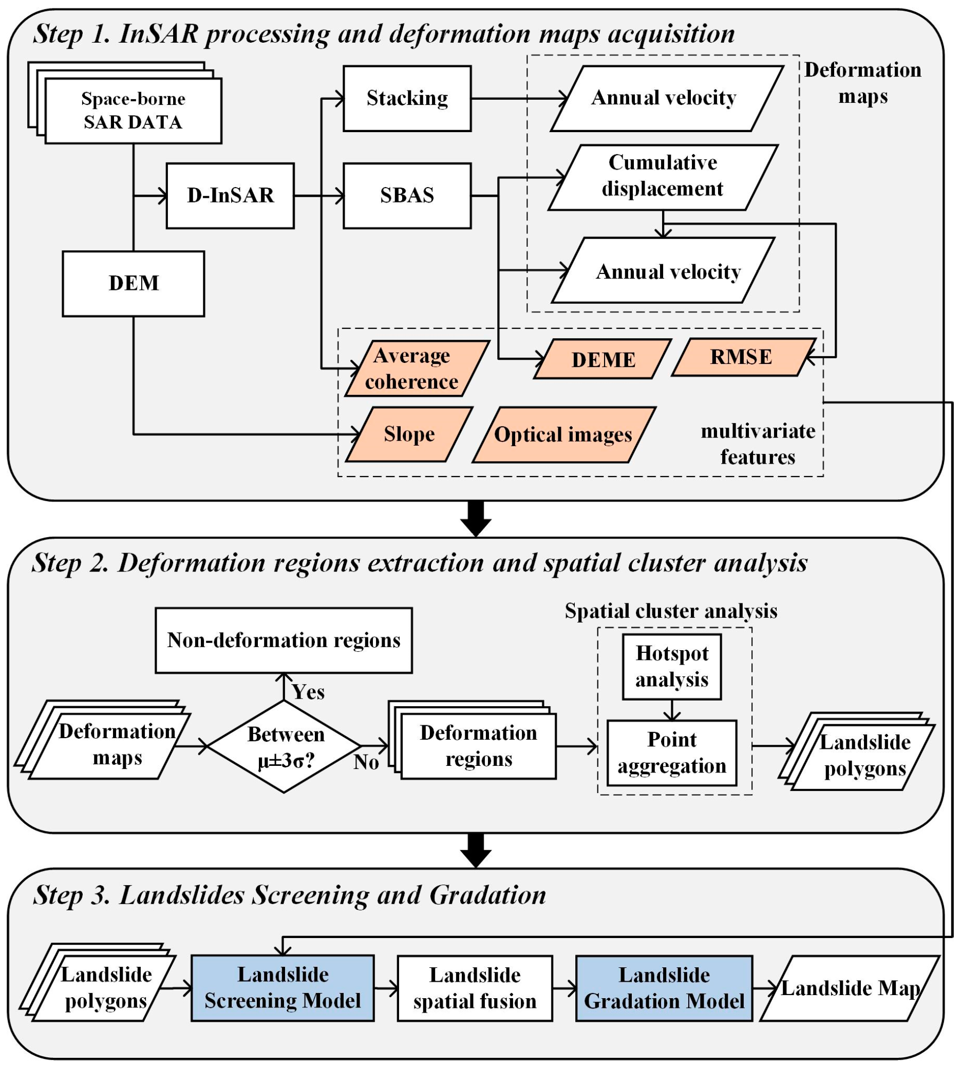
  • SBAS-InSAR and stacking-InSAR are combined to generate deformation maps in the study area, which can obtain more information to avoid the omission of landslides in the study area;
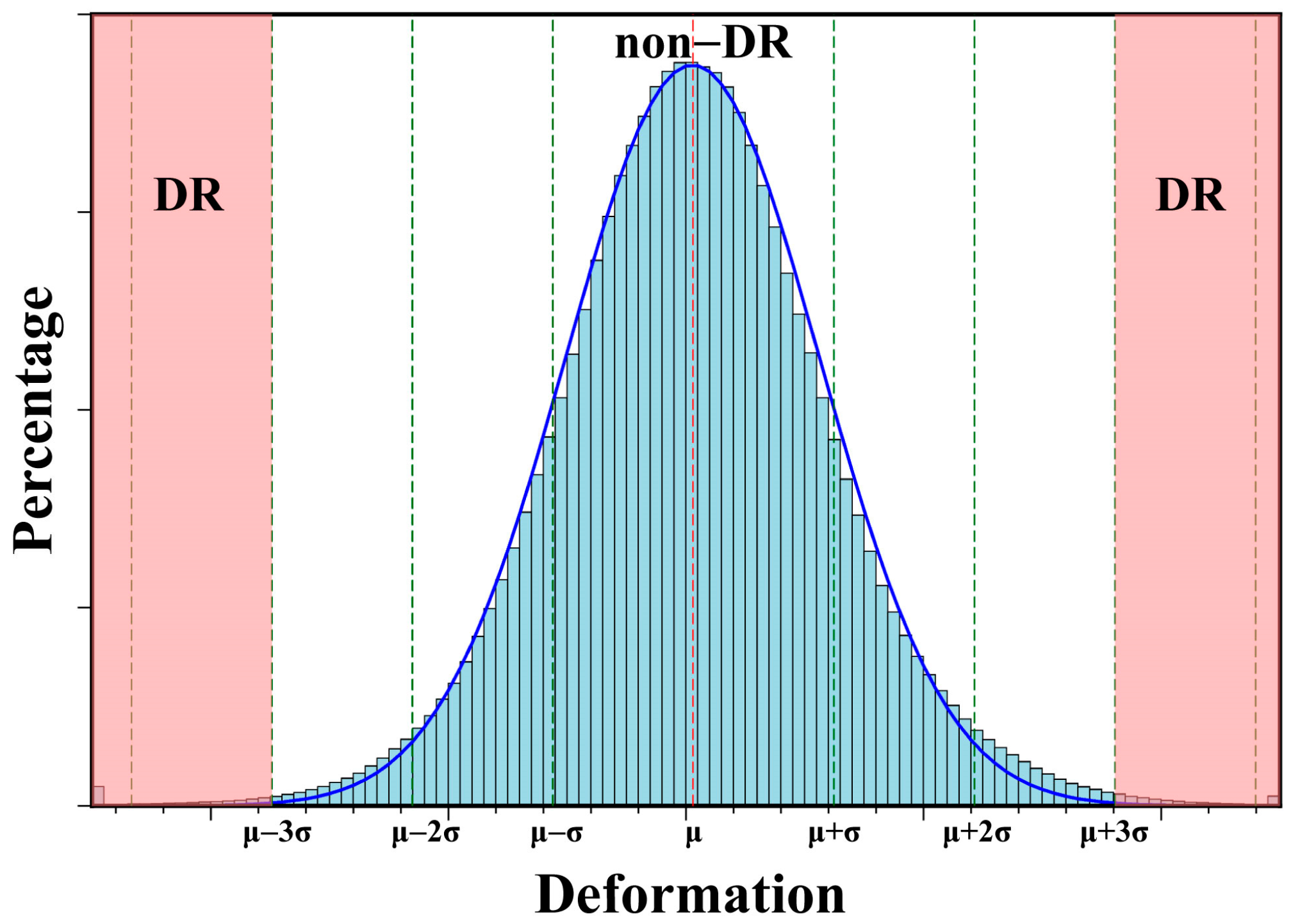
  • Statistical analysis and spatial cluster analysis are used to extract deformation regions and landslide polygons, which can provide a unified benchmark for landslide identification in different regions;
  • A landslides screening model (LSM) based on multivariate features is proposed to screen landslide polygons, which can reduce the interference of noise in landslide identification; and
  • A landslides gradation model (LGM) based on the signum function is proposed to divide screened landslides into four risk grades for geological disaster monitoring and risk assessment to provide effective information.
The structure of this paper is arranged as follows. In Section 2, we describe the principle and details of the proposed method. In Section 3, we introduce the experimental area. In Section 4, we demonstrate the specific implementation steps of the proposed method in the Jinsha River basin and verify the validity of the proposed model. In Section 5 and Section 6, we discuss the obtained results and present our conclusions.

2. Methods

In this section, we describe how to accurately and reliably identify potential landslides in low-coherence areas, such as alpine canyon areas and vegetation coverage areas. Figure 1 shows the workflow of the proposed method. The specific process can be divided into the following three parts.

2.1. InSAR Processing and Deformation Results Acquisition

Through D-InSAR processing, SBAS-InSAR processing, and stacking-InSAR processing, three deformation maps of the study area are obtained, including the annual velocity map obtained by SBAS, a time-series cumulative displacement map obtained by SBAS, and an annual velocity map obtained by stacking.
  • D-InSAR processing.
GMTSAR software [49] is used to process Sentinel-1 images to generate interferograms. Based on the principle of the shortest total temporal baseline, the super master image is selected for registration. The spatiotemporal baseline between each image is calculated according to precise orbit determination ephemerides, which are used to select interferogram pairs according to the SBAS-InSAR algorithm strategy. The interferograms are unwrapped using the statistical-cost network-flow algorithm for phase unwrapping (SNAPHU) [50,51]. The topographic phase is removed using a digital elevation model (DEM) from the Shuttle Radar Topography Mission [52].
2.
SBAS-InSAR processing.
The basic principle of SBAS-InSAR is to minimize the error and spatiotemporal decorrelation caused by the difference in viewing angles between interferogram pairs by setting the spatiotemporal baseline threshold, and the time-series deformation results are obtained by least square solution and singular value decomposition (SVD). Through the SBAS program encapsulated by GMTSAR, four results are obtained: annual velocity, cumulative displacement, root mean square error (RMSE) during linear deformation fitting, and estimated DEM error (DEME).
3.
Stacking-InSAR processing.
Stacking-InSAR can further weaken the influence of orbit, atmosphere, and terrain errors by weighting together N unwrapped interferograms [34,53]. Stacking-InSAR assumes that the annual velocity is the ratio of cumulative displacement to time and does not consider the distribution of other noise elements in the process of phase unwrapping with different interferograms; that is, only linear deformation is considered in the study area. The mainstream landslide sliding model assumes that the landslide moves along the steepest downhill slope [37], constituting a linear deformation model. Therefore, using stacking-InSAR technology to identify landslides is a more effective method. The annual velocity in the time series is calculated using Equation (1).
V s t a c k i n g = λ 4 π i = 1 N φ i Δ T i i = 1 N Δ T i 2
where V s t a c k i n g is the annual velocity in mm/yr, λ is the radar wavelength in millimeters, N is the number of interferogram pairs, φ i is the unwrapped interferometric phase, and Δ T i is the temporal baseline length of interferogram pairs in years.

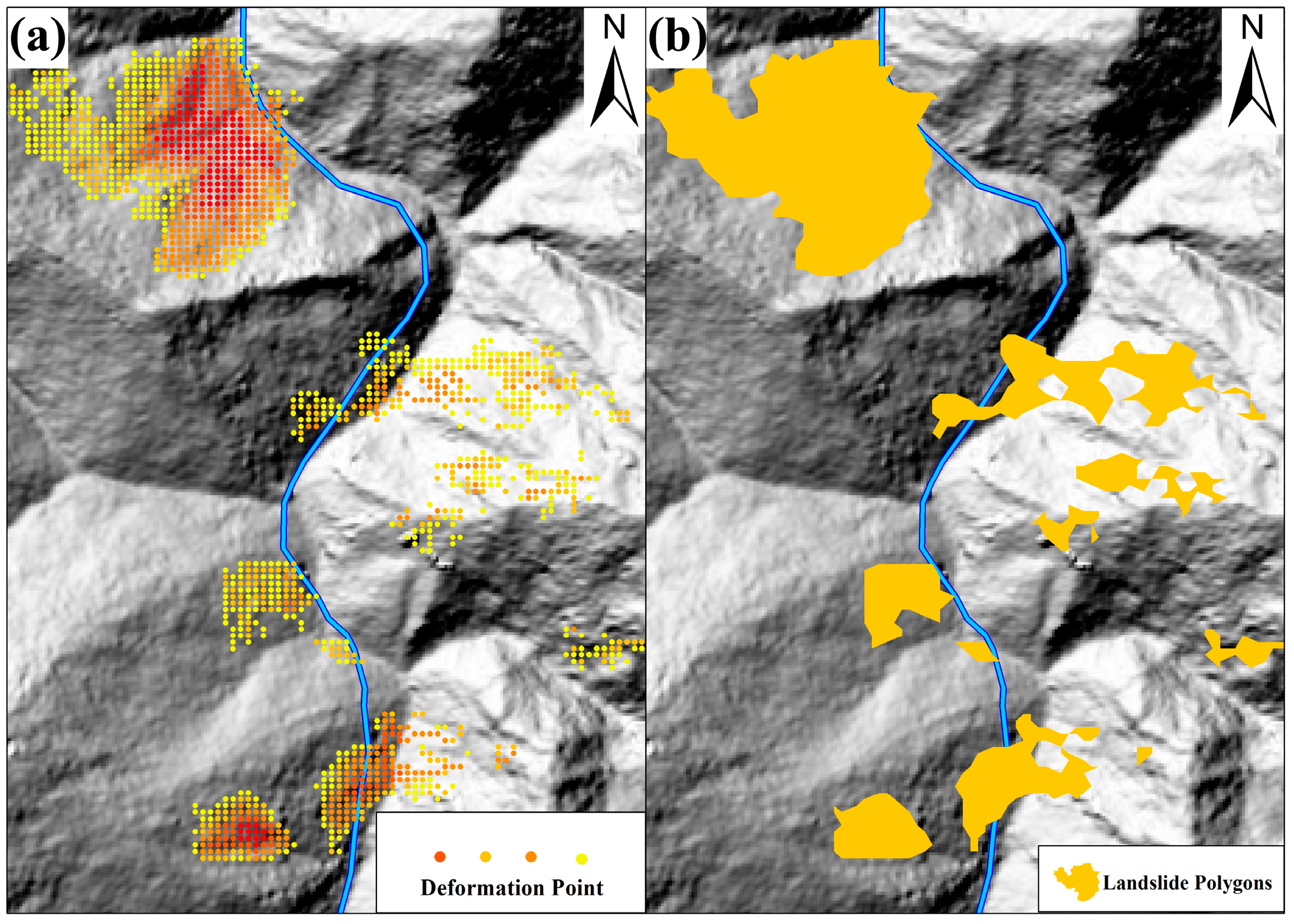
2.2. Deformation Region Extraction and Spatial Cluster Analysis

SBAS-InSAR considerably reduces the influence of spatiotemporal decorrelation and atmospheric delay by setting a baseline threshold and spatiotemporal filtering. Stacking-InSAR also weakens the influence of orbital error, terrain error, and atmospheric error in interferograms by stacking. The residual noise phase after application of the above noise reduction methods has random characteristics.
According to the central limit theorem, the distribution of a large number of random variables is close to the normal distribution. Based on the assumption of normal distribution, deformation regions and non-deformation regions are extracted from the statistical indicators (mean and standard deviation; μ and σ, respectively) of three deformation maps. Assuming that an area without any deformation, the results of surface deformation obtained by InSAR should obey the distribution of N(0,σ). Due to the existence of a series of noise reduction methods and random noise phases, the actual obtained distribution is close to the normal distribution (N(μ,σ)). For the normal distribution, the random variables distributed in the range of μ ± 3σ account for 99.74%. After calculating μ and σ of the deformation map according to this theory, the results outside the range of μ ± 3σ are categorized as deformation regions (DR), and the results within the range of μ ± 3σ are categorized as non-deformation regions (non-DR). The deformation regions map is obtained, as well as the distribution histogram of deformation results and its fitting normal distribution curve, as shown in Figure 2.
Spatial cluster analysis is a method to quickly screen points with aggregated deformation, which can remove the interference of discrete points. A landslide is a collection of clustered points, so the spatial cluster analysis method can be used to identify suspicious landslide areas in a deformation regions map. The hotspot analysis method based on the Getis-Ord Gi* statistics [54] and the point aggregation method are used for spatial cluster analysis to obtain landslide polygons in the study area. As a hypothesis-testing method, the hotspot analysis method judges whether deformation points are significantly aggregated by checking the difference between adjacent elements within the specified critical distance range; this method can identify spatial clusters with large deformation on a deformation regions map. The hotspot analysis method uses the Getis-Ord Gi* statistic [47] to determine the spatial aggregation of the deformation points. Equation (2) can calculate a value of Gi*(d) for each deformation point; the larger the absolute value of Gi*(d), the stronger the aggregation of deformation points. In the present study, the confidence of the hypothesis test is set to 0.99, and the corresponding critical value (|Gi*(d)|) of the deformation point is 2.58.
G i * ( d ) = j = 1 n i j x j + x i n i j x ¯ S * n n i j n i j 2 n 1
where n represents the total number of deformation points; nij represents the number of deformation points within the search distance (d) of the i-th deformation point (i = 1, 2, …, n; j = 1, 2, …, nij; j ≠ i); x represents the value of a deformation point (annual velocity and cumulative displacement); and x ¯ and S * represent the mean and standard deviation of all deformation point values, respectively. With a confidence of 0.99, if the |Gi*(d)| value of a deformation point is greater than 2.58, the deformation point is considered to have strong spatial aggregation.
After hotspot analysis, all feature points with high aggregation are extracted, but there are still a small number of discrete points. The point aggregation method is used to further eliminate these discrete points. The point aggregation method aggregates the points into faces by setting a certain distance threshold, which can extract landslide polygons with aggregation features on a deformation regions map, as shown in Figure 3.
Hotspot analysis and point aggregation are clustered based on the distance between deformation points. Selecting an appropriate distance threshold is the key to correctly identifying landslides. Using the smallest possible distance threshold for hotspot analysis and point aggregation can maximize the spatial differences between deformation point clusters.

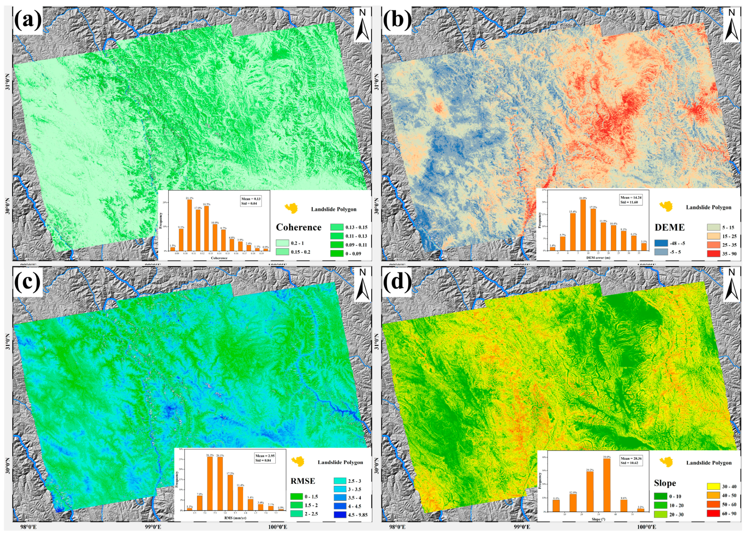
2.3. Landslide Screening Based on LSM

After spatial cluster analysis of the deformation regions extracted from these three InSAR results, the landslide polygons of each deformation result are obtained, although most are phase noise, not real landslides. To remove these noises, LSM-based multivariate features is proposed to screen all landslide polygons. Figure 4 shows LSM-screened landslide polygons based on six features: time-series average coherence (γmean) [55], DEME, RMSE, slope, area, and optical image features.
The time-series average coherence (γmean) from the coherence maps of all interferogram pairs is calculated by Equation (3).
γ mean = 1 1 m k = 1 m ( 1 γ k 2 γ k 2 + 1 )  
where γk is the coherence map of each interferogram pair, and m is the number of interferograms. DEME and RMSE are the results generated by the SBAS program encapsulated by GMTSAR software. According to the statistics [56], landslides mostly develop on terrain slopes in the range of 25° to 45°. The slope threshold of landslide polygons is set to 25°, and the average slope value is calculated based on DEM data. The area threshold is set to 0.1 km2 to screen landslide polygons larger than medium size. For each landslide polygon obtained based on SBAS-InSAR data, the μ and σ of the five indicators are calculated and used as thresholds to screen all landslide polygons. For landslide polygons obtained by stacking-InSAR, because there is no DEME and RMSE, only three indicators are used for screening: γmean, area, and slope. To avoid missing dangerous landslides, the landslide polygons with maximum deformation values outside the range of μ ± 6σ are also screened.
After the above processing steps, it is also necessary to observe whether the polygonal area of the landslide shows the topographic and geomorphic characteristics of landslides in optical images [57,58,59,60]. Unstable landslides usually exhibit some macroscopic features before sliding (downward gentle dip and unleveled phenomena; new gullies on the surface of landslides; loose soil and rocks in front of landslide and face the danger of river erosion; the surface of the landslide is bare and not covered by vegetation). Google Earth optical images are used to judge whether the landslide polygon has any of the above characteristics, and landslide polygons are further screened to obtain a landslide map of the study area.

2.4. Landslide Gradation Based on LGM

After the above screening process, the screened landslides are obtained based on the three deformation results and spatially fused to obtain a landslide map of the study area, as shown in Figure 5.
It is necessary to evaluate the grade of the landslide to estimate the risk of disasters after obtaining the basic landslide information. In this paper, LGM based on the signum function is proposed to grade screened landslides, as shown in Figure 6.
The signum function adds a graded label corresponding to three deformation maps to each landslide according to Equation (4).
c l a s s i f y i = { 1 , others 0 ,     μ 6 σ < m a x < μ + 6 σ                                      
g r a d e = i = 1 3 c l a s s i f y i
Here, μ ± 6σ is set as the threshold of deformation gradation [61]; max refers to the maximum value for the positive value of LOS direction and the minimum value for the negative value of LOS direction. The gradation result of each landslide (Equation (5)) is obtained by superimposing graded labels corresponding to three deformation maps.
According to the gradation results, the screened landslides are divided into four grades: L-I, L-II, L-III, and L-IV. The higher the grade, the greater the degree of landslide sliding and the greater the risk of landslide disaster. It is necessary to strengthen the monitoring of high-grade landslides.

3. Study Area and Datasets
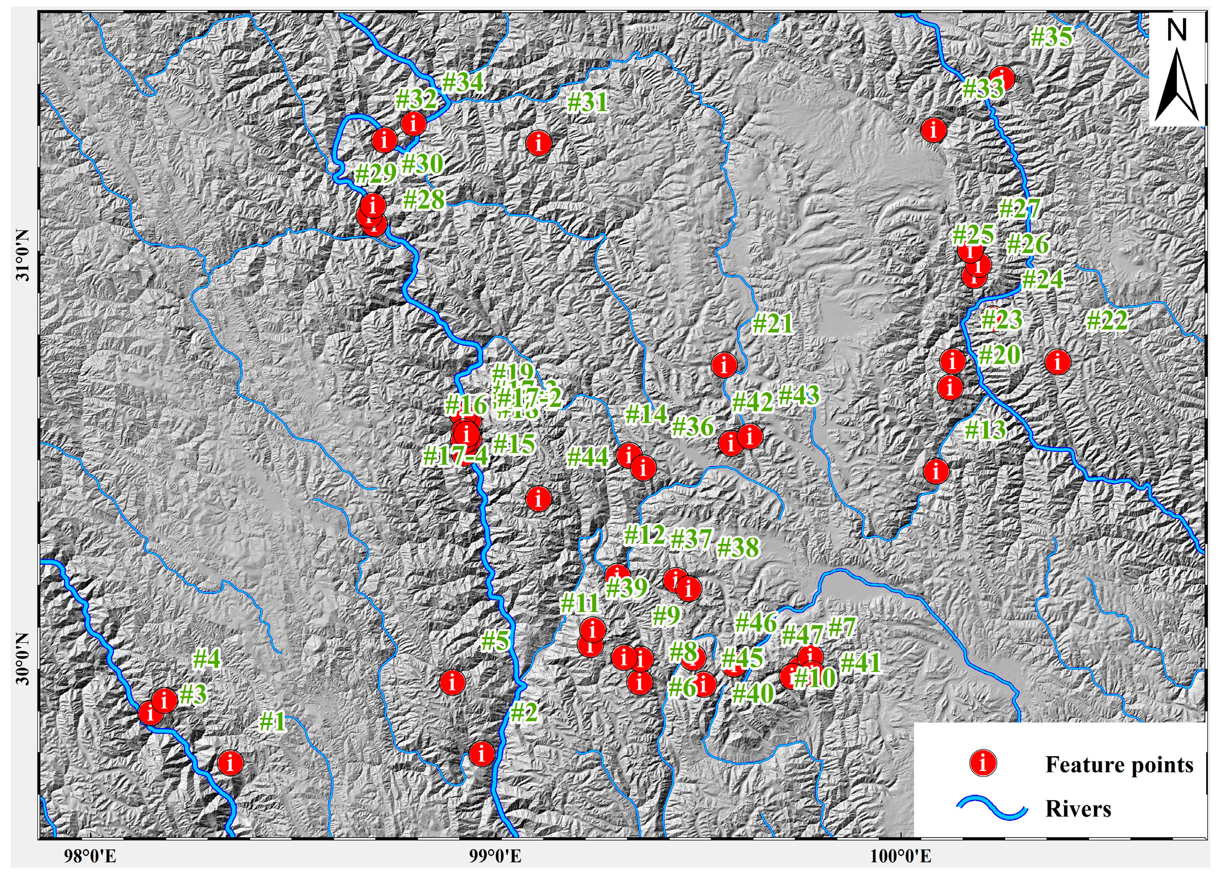
3.1. Study Area

The Jinsha River constitutes the upper reaches of the Yangtze River, which flows through the four provinces of Qinghai, Sichuan, Tibet, and Yunnan. It originates from the Tanggula Mountains and joins the Yangtze River in Yibin, Sichuan. The terrain of the Jinsha River basin is undulating, and the drop of up as much as 3300 m provides considerable kinetic energy to the river water. Under the impact of the river and the uplift of the Qinghai-Tibet Plateau, a “V”-shaped structure of alpine valleys is formed. The Jinsha River basin is a high-incidence area of landslides, with many landslides, collapses, and blockages recorded throughout history.
The study area is located in the upper section of the Jinsha River basin, as shown in Figure 7. The latitude and longitude ranges are 97°52′E–100°46′E and 29°33′N–31°36′N, respectively, and the altitude span is 2300–6000 m, covering an area of 46,157 km2. The study area comprises typical alpine and canyon terrain, with dense vegetation coverage, numerous snow-capped mountains, and densely developed rivers. The climatic zones of the study area are the temperate humid climate zone of the western Sichuan Plateau and the temperate semi-humid climate zone of the eastern Tibetan Plateau [36], and vertical climate change is obvious, depending on the altitude image. The study area experiences considerable rainfall in summer, with rainfall lasts for a long time due to the large area of the watershed. The flood season occurs from late June to mid-October, especially from July to September. The temperature difference between day and night in the study area is large, and the effect of freeze–thaw weathering is extremely strong. Coupled with river scouring, the stability of the rock mass in the basin is poor.

3.2. Datasets

The SAR data used in this paper comprise Sentinel-1 images. For the selected research area, we intended to used ascending and descending images for joint observation to obtain more landslide information. After actual processing, serious decorrelation of the descending images was observed, and more effective information could not be obtained. Therefore, we only used ascending images to demonstrate the proposed method.
Sentinel-1 images and the corresponding precise orbit determination ephemeris files were obtained from the European Space Agency (ESA) website. The data acquisition period was from September 2018 to February 2021, with 76 scenes in total. Details of used data and relevant processing parameters are presented in Table 1, and the combinations of interferogram pairs are shown in Figure 8. The cropped DEM data of the research area were obtained from the official website of GMTSAR software, with a 1 s arc resolution corresponding to 30 m ground resolution.

4. Results and Analysis

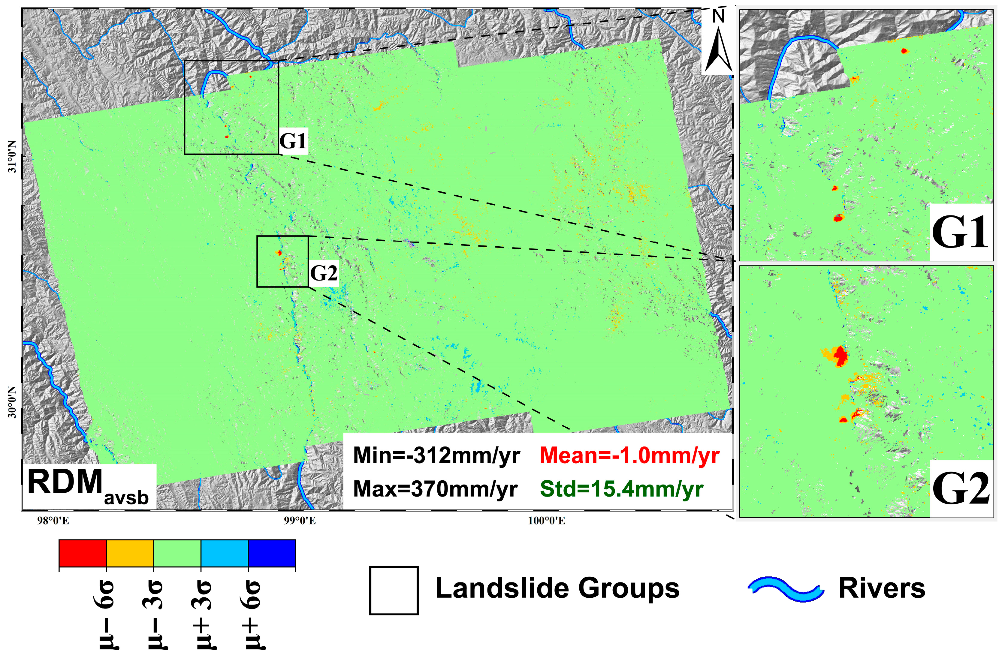
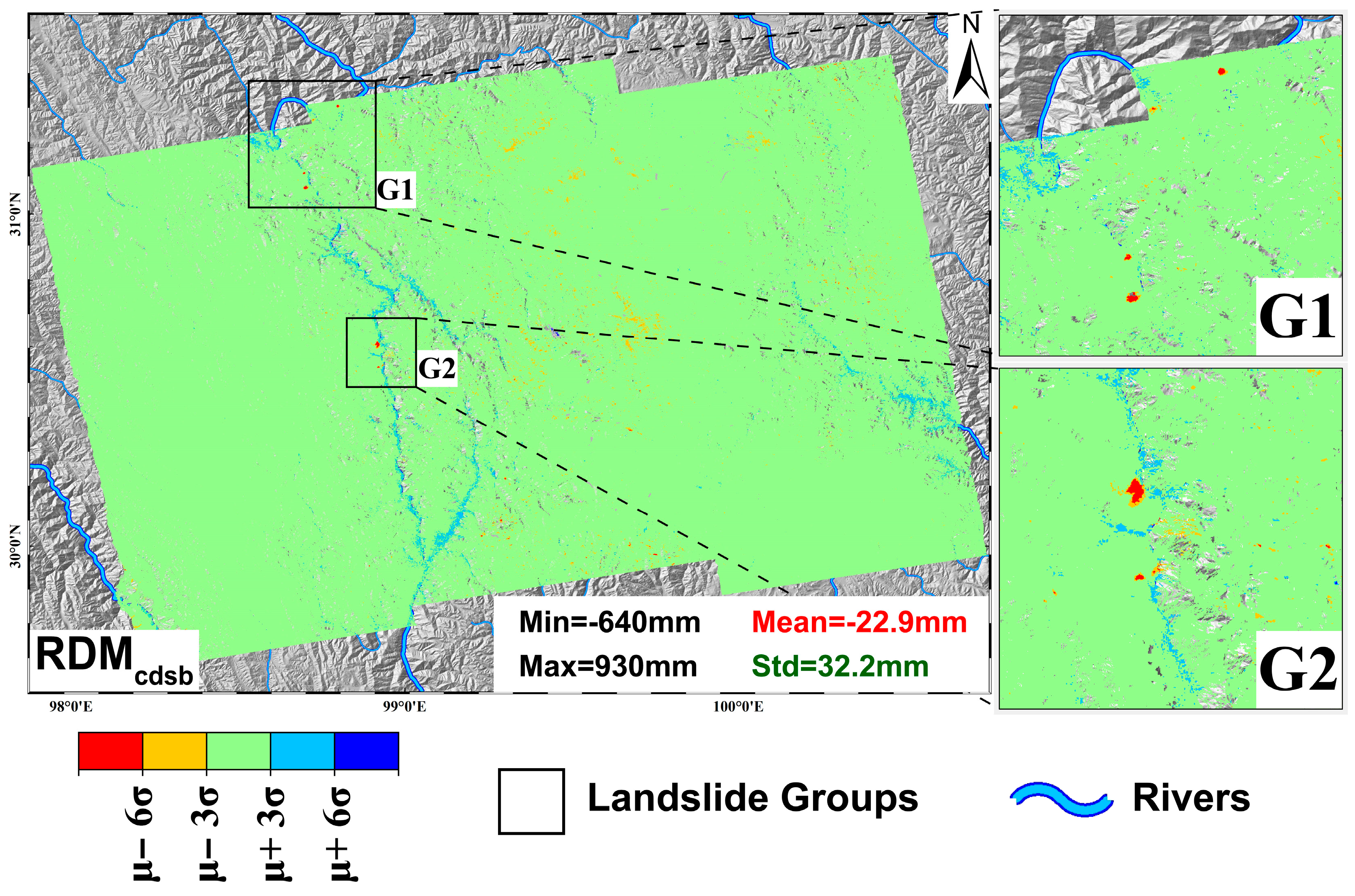
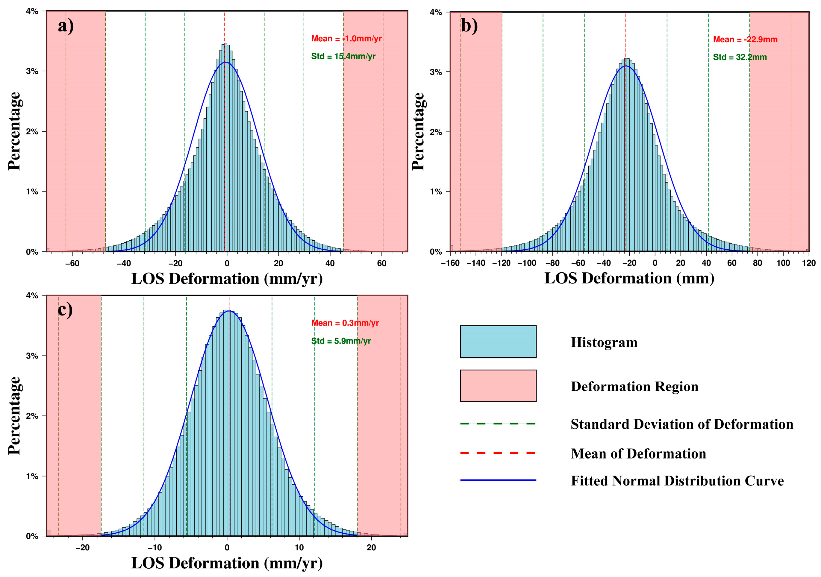
4.1. Deformation Results

Using the SBAS-InSAR and stacking-InSAR methods, three deformation maps were obtained from the ascending data in the study area, as shown in Figure 9, Figure 10 and Figure 11. Combining the three results revealed two obvious landslide groups: G1 and G2; landslide group G1 comprises four landslides, including the Baige landslide, and landslide group G2 comprises several landslides, including the Xiongba ancient landslide. These results are consistent with previous studies [18,38,39]. The distribution histograms of the three deformation maps were generated (Figure 12), and the normal distribution curves were fitted according to the μ and σ of the three results. The fitted normal distribution curves of the three results are in agreement with the distribution histogram.

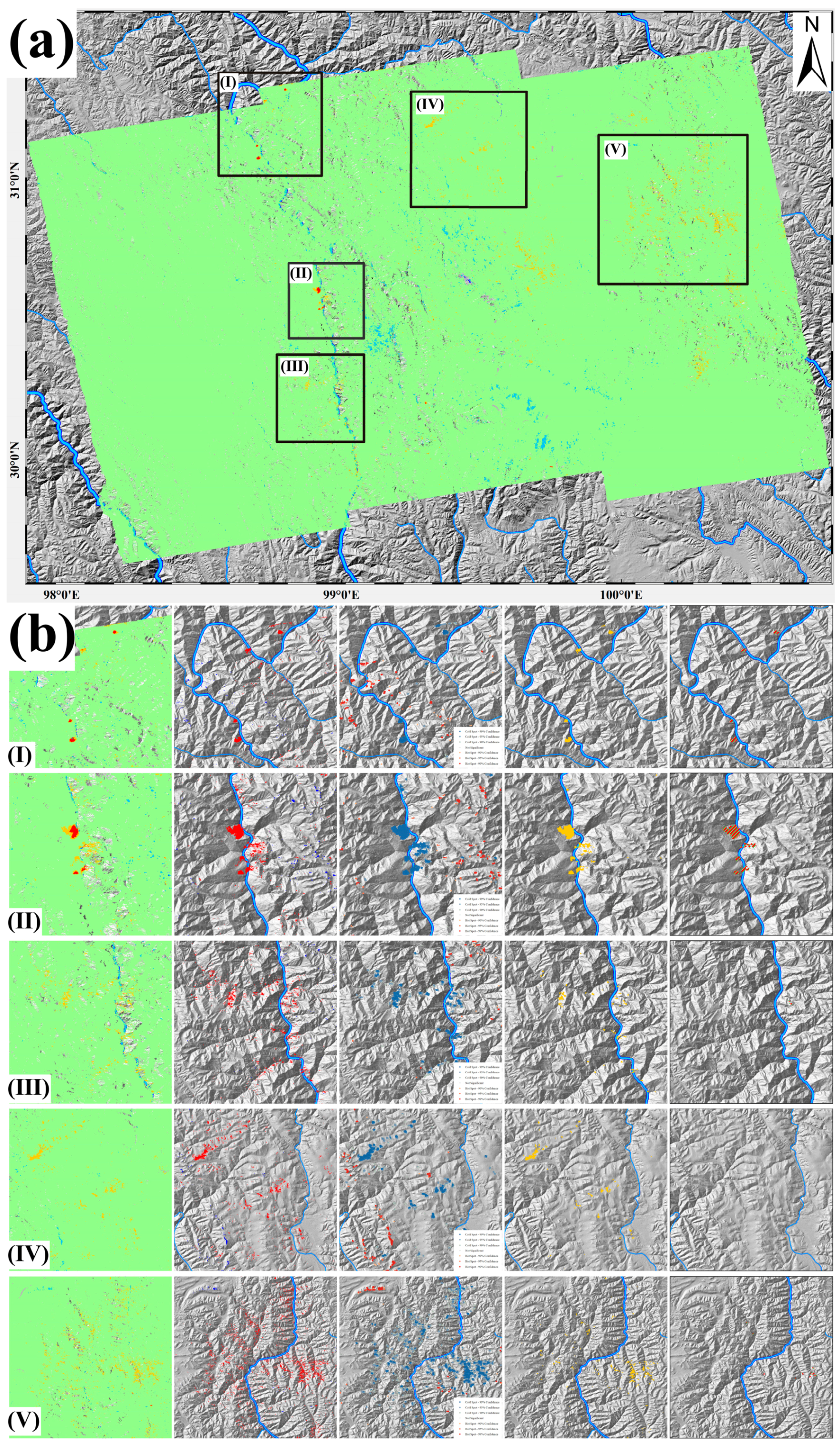
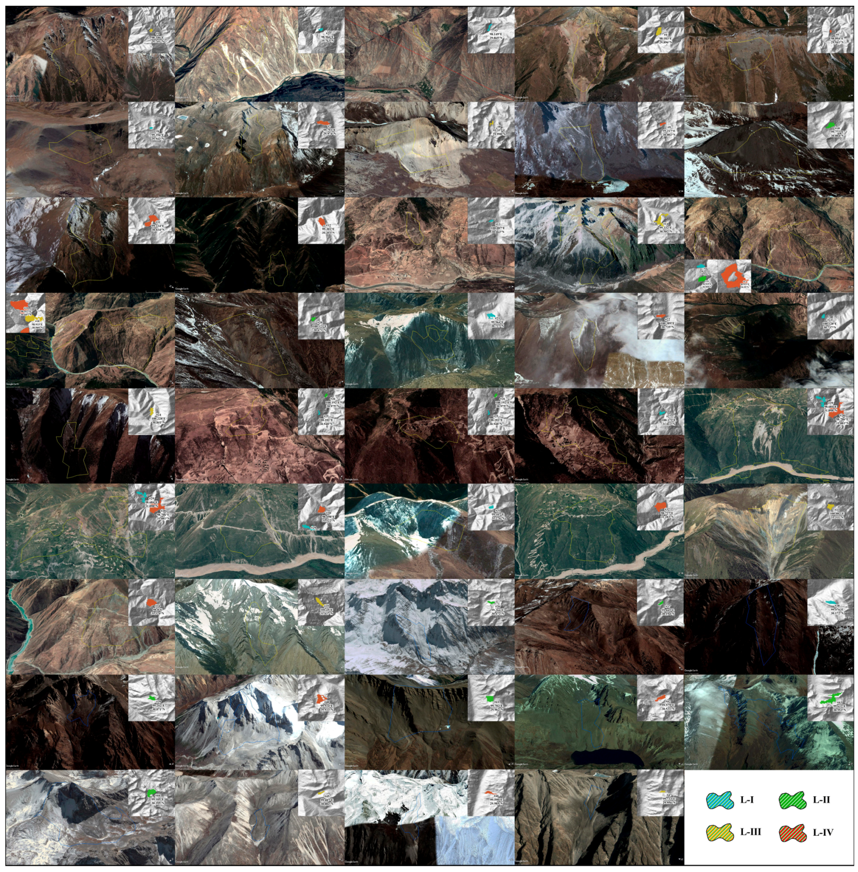
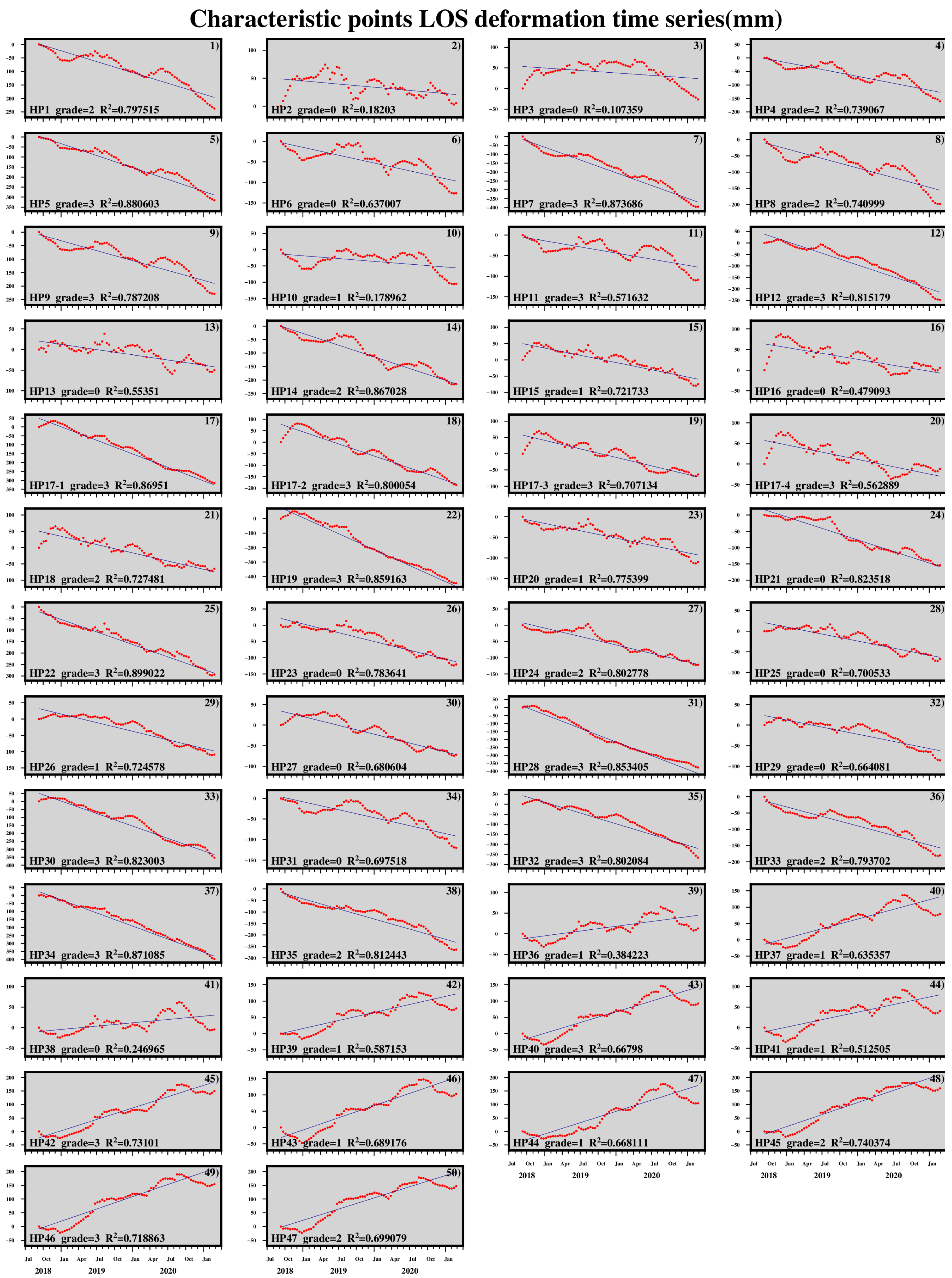
4.2. Landslides Identification and Gradation

Figure 13 shows the process of spatial cluster analysis and landslide screening on annual velocity map obtained by SBAS. Five areas presented with obvious deformation, as shown in Figure 13a, numbered as (I)–(V). The deformation regions were first extracted using statistical analysis, as shown in Figure 13b second column, with negative values in red and positive values in blue. Then, spatial cluster analysis was performed to extract landslide polygons from deformation regions, as shown in Figure 13b third column and fourth column. A total of 72,171 deformation points were identified in the deformation regions map. Via hotspot analysis, 37,674 deformation points with strong aggregation characteristics were extracted, of which 17,356 were negative deformation points (dark blue) and 20,318 were positive deformation points (dark red). Via point aggregation analysis, 595 landslide polygons with negative values were generated. Then, the proposed LSM was used to screen all landslide polygons, as shown in Figure 13b fifth column. The time-series average coherence map, DEME map, RMSE map, and slope map of the study area are shown in Figure 14. The landslide polygon statistics and model parameters are shown in Table 2. The landslide map includes 32 landslides obtained according to the steps outlined above.
Using the same method, 31 landslides were screened from 1011 landslide polygons on the cumulative displacement map obtained by SBAS, and 29 landslides were screened from 477 landslide polygons on the annual velocity map obtained by stacking. These landslides identified by three deformation maps were spatially fused to obtain the landslide map, which included 63 landslides with negative values. Then, an additional 32 landslides with positive values based on this method were included, and a complete landslide map containing 95 landslides was obtained. To reduce the repetitive workload, the optical image screening step that should have been performed before spatial fusion was performed after spatial fusion. Based on the macroscopic features of unstable landslides mentioned in Section 2.3, Google Earth optical images were used to confirm whether the screened landslides had corresponding macroscopic features. Ultimately, 47 landslides were identified, as shown in Figure 15.
These landslides were graded using the proposed LGM. After gradation, among the 47 landslides, 15 were identified as L-IV landslides, 10 as L-III landslides, 10 as L-II landslides, and 12 as L-I landslides. Among the 47 identified landslides, 13 landslides directly endangered villages. If a geological disaster occurs, the villages located below will be directly impacted. Therefore, it was also necessary to strengthen the monitoring of these 13 landslides.

4.3. Validation of Landslide Identification Results

To validate the landslide identification method proposed in this paper, two landslide groups (G1 and G2 in Figure 9) were chosen as the research objects to compare with the results obtained by other researchers. Figure 16a–d corresponds to the G2 landslide group, and Figure 16e,f corresponds to the G1 landslide group. The landslide boundaries identified in the present study were consistent with the landslide boundaries artificially identified by other researchers, and more landslide features can be observed: the pink line of landslide #19 in Figure 16 identifies the boundary reflected by the cumulative displacement map, which was significantly smaller than the blue and green boundaries, indicating that the landslide body was composed of a part of the continuous sliding body and a part of the seasonal sliding body; the pink and blue lines of landslides #17-1 and #17-2 in Figure 16d indicate that the landslide was composed of two independent sliding blocks; landslide #18 in Figure 16d and landslide #28 in Figure 16f indicate that stacking-InSAR can obtain more complete landslide boundary information than SBAS-InSAR, and the combined use of the two InSAR methods can solve the problem of omission or lack of landslide boundaries caused by decorrelation.
To validate the LGM proposed in this paper, feature points were selected among the 47 identified landslides, among which four feature points of landslide #17 were selected. Using the time-series cumulative displacement results obtained by SBAS-InSAR, the deformation on the time series of each feature point was extracted, as shown in Figure 17. The distribution of these 50 feature points is shown in Figure 18. According to the principle of least squares, the linear deformation velocity of each feature point was fitted, and the correlation coefficient (R2) between the fitted linear deformation velocity and the time series deformation was calculated. The R2 under different grades was quantified, and the statistical results are shown in Table 3. With increased deformation grade, the R2 of each landslide feature point increased significantly, indicating that the R2 is obviously positively correlated with the landslide grade. Furthermore, the R2 of the feature points can reflect the linear deformation trend of the landslide point. The larger the deformation degree and the stronger the linear deformation trend, the more urgent the need for landslide monitoring. The proposed LGM can provide a distinction basis for the monitoring of landslides in large areas.

5. Discussion

Frequent landslides in alpine canyon areas and vegetation coverage areas have attracted the research attention of scholars. Accurate identification of potential landslides and monitoring of high-risk landslides in these areas is an important task. Generally speaking, such areas are considerably affected by decorrelation (temporal decorrelation caused by vegetation coverage and spatial decorrelation caused by excessive deformation). In the present study, we combined SBAS-InSAR and stacking-InSAR to weaken the influence of decorrelation and avoid the omission of landslide identification by obtaining more data. In the process of landslide identification, accurate definition of the deformation region of landslides is very important. Based on the random characteristics of the phase noise and statistical analysis method, in the present study, we used the mean and three standard deviations of deformation results to distinguish between deformation regions and non-deformation regions to extract landslide deformation regions for subsequent landslide screening.
In the research presented in this paper, the spatial cluster analysis method was used to extract landslide polygons with clustering characteristics in deformation regions, an LSM based on multivariate features was proposed to screen the landslide polygons, and an LGM based on a signum function was proposed to grade the screened landslides. The proposed LSM uses the multivariate features of landslide polygons to evaluate the reliability of each landslide polygon as “true”, combined with optical image features to screen landslide polygons that are statistically excellent, effectively reducing false alarms of landslides. The proposed LGM uses the signum function to add results labels to each identified landslide and grade the landslides according to the degree of deformation, providing support for risk assessment of landslides in large areas and effectively avoiding waste of human and material resources. The landslide identification method proposed in this paper was automated and parameterized, which can minimize the identification error caused by human subjective factors.
Some of the landslide boundaries automatically identified in this paper were differed from real landslide boundaries. As shown in Figure 5 and Figure 15, landslide #17 comprised fusion of three landslides, the boundary of landslides #18 and #28 spanned the Jinsha River, and the boundary of landslide #33 was smaller than the real landslide boundary. A possible reason why the identified landslide boundary is larger than the real boundary range is that some noise points close to the landslide were classified into the landslide range during the spatial cluster analysis process. The possible reason that the identified landslide boundary is smaller than the real landslide boundary is the decorrelation caused by excessive deformation. To solve this problem, the next step was to introduce the idea of hydrological analysis to extract the ridge and valley lines of the study area, which were used to segment the landslide polygon, solving the problem of the landslide polygon crossing the terrain.

6. Conclusions

In this study, a method for landslide identification and gradation based on statistical analysis and spatial cluster analysis was proposed, which included a landslide screening model (LSM) based on multivariate features and a landslide gradation model (LGM) based on signum function. The proposed method was suitable for landslide hazard identification in low-coherence areas, such as alpine canyon areas and vegetation coverage areas, etc. It minimized the impact of phase noise, accurately identified landslides in large areas, and solved the problem of excessive false alarms and the considerable influence of decorrelation in the current InSAR landslide identification study. The proposed method can identify landslides with deformation characteristics and optical image characteristics in the study area and automatically extract the location, size, and boundary of potential landslides, which can provide support for geological disaster investigation departments.
Based on the landslide identification method proposed in this paper, 47 landslides were identified with obvious landslide characteristics in seven counties in the Jinsha River basin. These landslides were categorized as 15 L-IV landslides, 10 L-III landslides, 10 L-II landslides, and 12 L-I landslides using LGM. Geological disaster investigation agencies and local departments need to conduct real-time monitoring of 15 L-IV landslides and 13 landslides that endanger villages to prevent major geological disasters.
Our follow-up plan involves applying the proposed method to more areas in the southwestern mountainous region and to introduce the idea of hydrological analysis to solve the problem of landslide boundaries crossing terrain.

Author Contributions

Conceptualization, methodology, and software: H.D. (Huayan Dai) and W.T.; validation and formal analysis: H.Z. and H.D. (Huayang Dai); investigation: H.D. (Huayan Dai) and C.W.; resources and data curation: C.W., H.D. (Huayang Dai) and Y.T.; writing—original draft preparation: H.D. (Huayan Dai) and H.Z.; writing—review and editing: H.Z., Y.T. and H.D. (Huayan Dai); visualization: W.T. and L.Z.; supervision and project administration: H.Z. and Y.T. All authors have read and agreed to the published version of the manuscript.

Funding

This paper was funded by the National Natural Science Foundation of China, Grant No. 41930110.

Data Availability Statement

Not applicable.

Acknowledgments

The authors are grateful to the European Space Agency for providing Sentinel-1 A data and the SRTM for providing DEM data. In addition, the authors thank GMTSAR open source software for support and Google Earth for providing optical images.

Conflicts of Interest

The authors declare no conflict of interest.

References

  1. Lewkowicz, A.G.; Way, R.G. Extremes of summer climate trigger thousands of thermokarst landslides in a High Arctic environment. Nat. Commun. 2019, 10, 1329. [Google Scholar] [CrossRef] [PubMed]
  2. Guthrie, R.H. The effects of logging on frequency and distribution of landslides in three watersheds on Vancouver Island, British Columbia. Geomorphology 2002, 43, 273–292. [Google Scholar] [CrossRef]
  3. Achache, J. Applicability of SAR Interferometry for operational monitoring of landslides. In Proceedings of the Second Ers Applications Workshop, London, UK, 6–8 December 1995. [Google Scholar]
  4. Dabbiru, L.; Aanstoos, J.V.; Hasan, K.; Younan, N.H.; Wei, L. Landslide detection on earthen levees with X-band and L-band radar data. In Proceedings of the Applied Imagery Pattern Recognition Workshop, Washington, DC, USA, 23–25 October 2013. [Google Scholar]
  5. Zhao, C.; Liu, X.; Zhang, Q.; Peng, J.; Xu, Q. Research on Loess Landslide Identification, Monitoring and Failure Mode with InSAR Technique in Heifangtai, Gansu. Geomat. Inf. Sci. Wuhan Univ. 2019, 44, 996–1007. [Google Scholar]
  6. Ferretti, A.; Prati, C. Nonlinear subsidence rate estimation using permanent scatterers in differential SAR interferometry. IEEE Trans. Geosci. Remote Sens. 2000, 38, 2202–2212. [Google Scholar] [CrossRef]
  7. Ferretti, A.; Prati, C.; Rocca, F. Permanent scatterers in SAR interferometry. IEEE Trans. Geosci. Remote Sens. 2001, 39, 8–20. [Google Scholar] [CrossRef]
  8. Ferretti, A.; Fumagalli, A.; Novali, F.; Prati, C.; Rucci, A. A New Algorithm for Processing Interferometric Data-Stacks: SqueeSAR. IEEE Trans. Geosci. Remote Sens. 2011, 49, 3460–3470. [Google Scholar] [CrossRef]
  9. Berardino, P.; Fornaro, G.; Lanari, R.; Sansosti, E. A New Algorithm for Surface Deformation Monitoring Based on Small Baseline Differential SAR Interferograms. IEEE Trans. Geosci. Remote Sens. 2002, 40, 2375–2383. [Google Scholar] [CrossRef]
  10. Lanari, R.; Mora, O.; Manunta, M.; Mallorquí, J.J.; Sansosti, E. A small-baseline approach for investigating deformations on full-resolution differential SAR interferograms. IEEE Trans. Geosci. Remote Sens. 2004, 42, 1377–1386. [Google Scholar] [CrossRef]
  11. Hooper, A. A new method for measuring deformation on volcanoes and other natural terrains using InSAR persistent scatterers. Geophys. Res. Lett. 2004, 31, L23611. [Google Scholar] [CrossRef]
  12. Sandwell, D.T.; Price, E.J. Phase gradient approach to stacking interferograms. J. Geophys. Res. Solid Earth 1998, 103, 30183–30204. [Google Scholar] [CrossRef]
  13. Zebker, H.A.; Villasenor, J. Decorrelation in interferometric radar echoes. IEEE Trans. Geosci. Remote Sens. 1992, 30, 950–959. [Google Scholar] [CrossRef] [Green Version]
  14. Hanssen, R.F. Radar Interferometry; Springer: Berlin/Heidelberg, Germany, 2001. [Google Scholar]
  15. Goldstein, R. Atmospheric limitations to repeat-track radar interferometry. Geophys. Res. Lett. 2013, 22, 2517–2520. [Google Scholar]
  16. Pepe, A.; Berardino, P.; Bonano, M.; Euillades, L.D.; Lanari, R. SBAS-Based Satellite Orbit Correction for the Generation of DInSAR Time-Series: Application to RADARSAT-1 Data. IEEE Trans. Geosci. Remote Sens. 2011, 49, 5150–5165. [Google Scholar] [CrossRef]
  17. Gabriel, A.K.; Goldstein, R.M.; Zebker, H.A. Mapping small elevation changes over large areas: Differential radar interferometry. J. Geophys. Res. Solid Earth 1989, 94, 9183–9191. [Google Scholar] [CrossRef]
  18. Liu, X.; Zhao, C.; Zhang, Q.; Yin, Y.; Lu, Z.; Samsonov, S.; Yang, C.; Wang, M.; Tomas, R. Three-dimensional and long-term landslide displacement estimation by fusing C- and L-band SAR observations: A case study in Gongjue County, Tibet, China. Remote Sens. Environ. 2021, 267, 112745. [Google Scholar] [CrossRef]
  19. Burrows, K.; Walters, R.J.; Milledge, D.; Spaans, K.; Densmore, A.L. A New Method for Large-Scale Landslide Classification from Satellite Radar. Remote Sens. 2019, 11, 237. [Google Scholar] [CrossRef]
  20. Hu, X.; Wang, T.; Pierson, T.C.; Lu, Z.; Kim, J.; Cecere, T.H. Detecting seasonal landslide movement within the Cascade landslide complex (Washington) using time-series SAR imagery. Remote Sens. Environ. 2016, 187, 49–61. [Google Scholar] [CrossRef]
  21. Chen, L.; Zhao, C.; Kang, Y.; Chen, H.; Yang, C.; Li, B.; Liu, Y.; Xing, A. Pre-Event Deformation and Failure Mechanism Analysis of the Pusa Landslide, China with Multi-Sensor SAR Imagery. Remote Sens. 2020, 12, 856. [Google Scholar] [CrossRef]
  22. Wang, J.; Wang, C.; Xie, C.; Zhang, H.; Tang, Y.; Zhang, Z.; Shen, C. Monitoring of large-scale landslides in Zongling, Guizhou, China, with improved distributed scatterer interferometric SAR time series methods. Landslides 2020, 17, 1777–1795. [Google Scholar] [CrossRef]
  23. Tang, Y.; Zhang, Z.; Wang, C.; Zhang, H.; Wu, F.; Liu, M. Characterization of the giant landslide at Wenjiagou by the insar technique using TSX-TDX CoSSC data. Landslides 2015, 12, 1015–1021. [Google Scholar] [CrossRef]
  24. Tang, Y.; Zhang, Z.; Wang, C.; Zhang, H.; Wu, F.; Zhang, B.; Liu, M. The deformation analysis of Wenjiagou giant landslide by the distributed scatterer interferometry technique. Landslides 2018, 15, 347–357. [Google Scholar] [CrossRef]
  25. Hilley, G.E.; Burgmann, R.; Ferretti, A.; Novali, F.; Rocca, F. Dynamics of slow-moving landslides from permanent scatterer analysis. Science 2004, 304, 1952–1955. [Google Scholar] [CrossRef] [PubMed] [Green Version]
  26. Zhao, C.; Lu, Z.; Zhang, Q.; de la Fuente, J. Large-area landslide detection and monitoring with ALOS/PALSAR imagery data over Northern California and Southern Oregon, USA. Remote Sens. Environ. 2012, 124, 348–359. [Google Scholar] [CrossRef]
  27. Xiao-jun, S.; Yi, Z.; Xing-min, M.; Dong-xia, Y.; Jin-hui, M.; Fu-yun, G.; Zi-qiang, Z.; Rehman, M.U.; Khalid, Z.; Guan, C.; et al. Landslide mapping and analysis along the China-Pakistan Karakoram Highway based on SBAS-InSAR detection in 2017. J. Mt. Sci.-Engl. 2021, 18, 2540–2564. [Google Scholar]
  28. Tofani, V.; Raspini, F.; Catani, F.; Casagli, N. Persistent Scatterer Interferometry (PSI) Technique for Landslide Characterization and Monitoring. Remote Sens. 2013, 5, 1045–1065. [Google Scholar] [CrossRef]
  29. Ren, T.; Gong, W.; Gao, L.; Zhao, F.; Cheng, Z. An Interpretation Approach of Ascending-Descending SAR Data for Landslide Identification. Remote Sens. 2022, 14, 1299. [Google Scholar] [CrossRef]
  30. Qu, T.; Lu, P.; Liu, C.; Wan, H. Application of Time Series Insar Technique for Deformation Monitoring of Large-Scale Landslides in Mountainous Areas of Western China. Int. Arch. Photogramm. Remote Sens. Spat. Inf. Sci. 2016, 41, 89–91. [Google Scholar] [CrossRef]
  31. Bozzano, F.; Mazzanti, P.; Esposito, C.; Moretto, S.; Rocca, A. Potential of satellite InSAR monitoring for landslide Failure Forecasting. In Landslides and Engineered Slopes. Experience, Theory and Practice; CRC Press: Boca Raton, FL, USA, 2016; pp. 523–530. [Google Scholar]
  32. Jin, J.; Chen, G.; Meng, X.; Zhang, Y.; Shi, W.; Li, Y.; Yang, Y.; Jiang, W. Prediction of river damming susceptibility by landslides based on a logistic regression model and InSAR techniques: A case study of the Bailong River Basin, China. Eng. Geol. 2022, 299, 106562. [Google Scholar] [CrossRef]
  33. Moretto, S.; Bozzano, F.; Mazzanti, P. The Role of Satellite InSAR for Landslide Forecasting: Limitations and Openings. Remote Sens. 2021, 13, 3735. [Google Scholar] [CrossRef]
  34. Nof, R.N.; Baer, G.; Eyal, Y.; Novali, F. Current surface displacement along the carmel Fault system in Israel from InSAR stacking and PSInSAR. Isr. J. Earth Sci. 2008, 57, 71–86. [Google Scholar] [CrossRef]
  35. Wright, T.; Parsons, B.; Fielding, E. Measurement of interseismic strain accumulation across the North Anatolian Fault by satellite radar interferometry. Geophys. Res. Lett. 2001, 28, 2117–2120. [Google Scholar] [CrossRef]
  36. Zhang, L.; Dai, K.; Deng, J.; Ge, D.; Liang, R.; Li, W.; Xu, Q. Identifying Potential Landslides by Stacking-InSAR in Southwestern China and Its Performance Comparison with SBAS-InSAR. Remote Sens. 2021, 13, 3662. [Google Scholar] [CrossRef]
  37. Jia, H.; Wang, Y.; Ge, D.; Deng, Y.; Wang, R. InSAR Study of Landslides: Early Detection, Three-Dimensional, and Long-Term Surface Displacement Estimation—A Case of Xiaojiang River Basin, China. Remote Sens. 2022, 14, 1759. [Google Scholar] [CrossRef]
  38. Liu, X.; Zhao, C.; Zhang, Q.; Lu, Z.; Liu, C. Integration of Sentinel-1 and ALOS/PALSAR-2 SAR datasets for mapping active landslides along the Jinsha River corridor, China. Eng. Geol. 2021, 284, 106033. [Google Scholar] [CrossRef]
  39. Zhang, J.; Zhu, W.; Cheng, Y.; Li, Z. Landslide Detection in the Linzhi–Ya’an Section along the Sichuan–Tibet Railway Based on InSAR and Hot Spot Analysis Methods. Remote Sens. 2021, 13, 3566. [Google Scholar] [CrossRef]
  40. Anna, B.; Lorenzo, S.; Marta, B.; Oriol, M.; Silvia, B.; Gerardo, H.; Michele, C.; Roberto, S.; Elena, G.; Rosa, M. A Methodology to Detect and Update Active Deformation Areas Based on Sentinel-1 SAR Images. Remote Sens. 2017, 9, 1002. [Google Scholar]
  41. Aslan, G.; Foumelis, M.; Raucoules, D.; De Michele, M.; Bernardie, S.; Cakir, Z. Landslide Mapping and Monitoring Using Persistent Scatterer Interferometry (PSI) Technique in the French Alps. Remote Sens. 2020, 12, 1305. [Google Scholar] [CrossRef]
  42. Navarro, J.; Tomás, R.; Barra, A.; Pagán, J.I.; Crosetto, M. ADAtools: Automatic Detection and Classification of Active Deformation Areas from PSI Displacement Maps. Int. J. Geo-Inf. 2020, 9, 584. [Google Scholar] [CrossRef]
  43. Crippa, C.; Valbuzzi, E.; Frattini, P.; Crosta, G.B.; Spreafico, M.C.; Agliardi, F. Semi-automated regional classification of the style of activity of slow rock-slope deformations using PS InSAR and SqueeSAR velocity data. Landslides 2021, 18, 2445–2463. [Google Scholar] [CrossRef]
  44. Tomás, R.; Pagán, J.I.; Navarro, J.A.; Cano, M.; Casagli, N. Semi-Automatic Identification and Pre-Screening of Geological-Geotechnical Deformational Processes Using Persistent Scatterer Interferometry Datasets. Remote Sens. 2019, 11, 1675. [Google Scholar] [CrossRef]
  45. Wang, S.; Zhuang, J.; Mu, J.; Zheng, J.; Zhan, J.; Wang, J.; Fu, Y. Evaluation of landslide susceptibility of the Ya’an-Linzhi section of the Sichuan-Tibet Railway based on deep learning. Environ. Earth Sci. 2022, 81, 250. [Google Scholar] [CrossRef]
  46. Meghanadh, D.; Maurya, V.K.; Tiwari, A.; Dwivedi, R. A multi-criteria landslide susceptibility mapping using deep multi-layer perceptron network: A case study of Srinagar-Rudraprayag region (India). Adv. Space Res. 2022, 69, 1883–1893. [Google Scholar] [CrossRef]
  47. Getis, A.; Ord, J.K. The Analysis of Spatial Association by Use of Distance Statistics. Geogr. Anal. 1992, 24, 127–145. [Google Scholar] [CrossRef]
  48. Ping, L.U.; Casagli, N.; Catani, F.; Tofani, V. Persistent Scatterers Interferometry Hotspot and Cluster Analysis (PSI-HCA) for detection of extremely slow-moving landslides. Int. J. Remote Sens. 2012, 33, 466–489. [Google Scholar]
  49. Sandwell, D.; Mellors, R.; Tong, X.; Wei, M.; Wessel, P. Open radar interferometry software for mapping surface Deformation. EOS Trans. Am. Geophys. Union 2013, 92, 234. [Google Scholar] [CrossRef] [Green Version]
  50. Chen, C.W.; Zebker, H.A. Two-dimensional phase unwrapping with use of statistical models for cost functions in nonlinear optimization. J. Opt. Soc. Am. A 2001, 18, 338–351. [Google Scholar] [CrossRef]
  51. Chen, C.W.; Zebker, H.A. Phase Unwrapping for Large SAR Interferograms: Statistical Segmentation and Generalized Network Models. IEEE Trans. Geosci. Remote Sens. 2002, 40, 1709–1719. [Google Scholar] [CrossRef]
  52. Farr, T.G.; Rosen, P.A.; Caro, E.; Crippen, R.; Duren, R.; Hensley, S.; Kobrick, M.; Paller, M.; Rodriguez, E.; Roth, L.; et al. The shuttle radar topography mission. Rev. Geophys. 2007, 45, RG2004. [Google Scholar] [CrossRef]
  53. Liu, Z.; Qiu, H.; Zhu, Y.; Liu, Y.; Yang, D.; Ma, S.; Zhang, J.; Wang, Y.; Wang, L.; Tang, B. Efficient Identification and Monitoring of Landslides by Time-Series InSAR Combining Single- and Multi-Look Phases. Remote Sens. 2022, 14, 1026. [Google Scholar] [CrossRef]
  54. Ord, J.K.; Getis, A. Local Spatial Autocorrelation Statistics: Distributional Issues and an Application. Geogr. Anal. 1995, 27, 286–306. [Google Scholar] [CrossRef]
  55. Rosen, P.A.; Hensley, S.; Joughin, I.R.; Li, F.K.; Madsen, S.N.; Rodriguez, E.; Goldstein, R.M. Synthetic aperture radar interferometry—Invited paper. Proc. IEEE 2000, 88, 333–382. [Google Scholar] [CrossRef]
  56. Li, Y.; Meng, H.; Dong, Y.; Hu, S. Main Types and characterisitics of geo-hazard in China—Based on the results of geo-hazard survey in 290 counties. Chin. J. Geol. Hazard Control 2004, 15, 32–37. [Google Scholar]
  57. Wang, C.; Zhu, M.; Ma, Z.; He, Z.; Jiang, H.; Li, P.; Zhang, X.; Shi, J.; Chen, K.; Weng, T.; et al. Classification of Landslide Stability Based on Fine Topographic Features. In Proceedings of the 2020 17th International Computer Conference on Wavelet Active Media Technology and Information Processing (ICCWAMTIP), Chengdu, China, 18–20 December 2020; pp. 54–57. [Google Scholar]
  58. Wang, K.; Xu, H.; Zhang, S.; Wei, F.; Xie, W. Identification and Extraction of Geomorphological Features of Landslides Using Slope Units for Landslide Analysis. ISPRS Int. J. Geo-Inf. 2020, 9, 274. [Google Scholar] [CrossRef]
  59. Pawluszek, K. Landslide features identification and morphology investigation using high-resolution DEM derivatives. Nat. Hazards. 2019, 96, 311–330. [Google Scholar] [CrossRef]
  60. Doshida, S. The Difference in the Landslide Information by the Difference Between Geographical Features and Geological Conditions. In Advancing Culture of Living with Landslides; Mikos, M., Tiwari, B., Yin, Y., Sassa, K., Eds.; Springer International Publishing: Cham, Switzerland, 2017; pp. 999–1005. [Google Scholar]
  61. Luo, S.; Feng, G.; Xiong, Z.; Wang, H.; Zhao, Y.; Li, K.; Deng, K.; Wang, Y. An Improved Method for Automatic Identification and Assessment of Potential Geohazards Based on MT-InSAR Measurements. Remote Sens. 2021, 13, 3490. [Google Scholar] [CrossRef]
Figure 1. Flow chart of the proposed method.
Remotesensing 14 04504 g001
Figure 2. Distribution histogram of deformation results and its fitting normal distribution curve. The red dashed line represents the mean value of the deformation result, the green dashed line represents the standard deviation, and the light-red boxes represent the landslide deformation regions.
Remotesensing 14 04504 g002
Figure 3. Schematic diagram of point aggregation. (a) Deformation points extracted by hotspot analysis. (b) Landslide polygons generated by point aggregation.
Remotesensing 14 04504 g003
Figure 4. Landslide screening model.
Remotesensing 14 04504 g004
Figure 5. Landslide spatial fusion. (a) Landslide boundary identified by three deformation maps. (b) Landslide boundary after spatial fusion.
Remotesensing 14 04504 g005
Figure 6. Landslide gradation model. Red (L-IV) represents the highest grade of deformation, and blue (L-I) represents the lowest grade of deformation.
Remotesensing 14 04504 g006
Figure 7. Study area and SAR image coverage. The red box represents the data coverage area of Sentinel-1, the red point indicates the location of the Baige landslide, the pink point indicates the location of the Jinsha River Bridge, and the blue lines represent the river distribution in the study area, with the locations of the Jinsha River, Lancang River, and Yalong River marked. The inset in the upper-left corner shows the location of the study area within China.
Remotesensing 14 04504 g007
Figure 8. Temporal and spatial baseline of interferogram pairs.
Remotesensing 14 04504 g008
Figure 9. Annual velocity map obtained by SBAS.
Remotesensing 14 04504 g009
Figure 10. Time-series cumulative displacement map obtained by SBAS.
Remotesensing 14 04504 g010
Figure 11. Annual velocity map obtained by stacking.
Remotesensing 14 04504 g011
Figure 12. Distribution histogram of three deformation maps and its fitted normal distribution curve. (a) Annual velocity map obtained by SBAS. (b) Time-series cumulative displacement map obtained by SBAS. (c) Annual velocity map obtained by stacking.
Remotesensing 14 04504 g012
Figure 13. Spatial cluster analysis and landslide identification process. (a) Annual velocity map obtained by SBAS. (b) Landslide identification process in the five main deformation regions (I–V) of (a); each region corresponds to a row (I–V). The five columns of (b) are the enlarged deformation maps, the extracted DR, the hotspot analysis results, the polymerized landslide polygons, and the screened landslides, respectively.
Remotesensing 14 04504 g013
Figure 14. Landslide polygon statistics. (a) γmean with its landslide polygons statistic. (b) DEME with its landslide polygons statistic. (c) RMSE with its landslide polygons statistic. (d) Slope with its landslide polygons statistic.
Remotesensing 14 04504 g014
Figure 15. Optical images of identified landslides. The yellow line and blue lines represent landslides identified by the negative and positive deformation maps, respectively. The legend in the lower-right corner indicates the grade of landslides.
Remotesensing 14 04504 g015
Figure 16. Comparison with other research results; the deformation period time is marked. (a,b,e) Results obtained by Liu et al. [18,38]. (c) Results obtained by Zhang et al. [39]. (d,f) Results obtained in the present study. The legend of the original text in the figure was redrawn.
Remotesensing 14 04504 g016
Figure 17. Time-series deformation of each landslide characteristic point. The blue solid line is the fitted linear deformation velocity, and red dots represent time-series displacement. The name, grade, and linear fitting correlation coefficient of landslides are marked in each subgraph. Subfigures (1)–(50) correspond to the numbers of the characteristic points in Figure 18 respectively.
Remotesensing 14 04504 g017
Figure 18. Distribution of feature points.
Remotesensing 14 04504 g018
Table 1. Data information and related processing parameters.
SensorSentinel-1 A
Orbit DirectionAscending
Path Frame99–1280
Acquisition TimeSeptember 2018–February 2021
Number of Images76
Azimuth Angle247.3°
Incidence Angle34.34°
Ground Resolution5 m × 20 m
Multi-looked Ratio8:2
Temporal Baseline25 day
Spatial Baseline100 m
Number of Interferograms130
Table 2. Data statistics and threshold parameters.
FeaturesResearch AreaAverage within Polygons
MinMaxMeanStdMinMaxMeanStdThreshold
γmean0.070.970.230.120.080.40.130.04>0.13
RMSE (mm/yr)09.852.40.641.356.692.950.84<2.95
DEME (m)−48.490.611.610.1−12.5751.0514.2411.6−11.6~11.6
Slope (°)0832412.12.3858.7428.3610.62>25
Area (km2)----0.0034.1850.1240.289>0.1
Note: The first item represents the statistical data of each feature in the whole image range, and the second item represents the average statistical data of each feature in the landslide polygons.
Table 3. Relationship between landslide grade and correlation coefficient.
GradeNumPercentR2
MinMaxMean
L-I1225.53%0.110.820.55
L-II1021.28%0.180.780.59
L-III1021.28%0.700.870.77
L-IV1531.91%0.570.900.80
Publisher’s Note: MDPI stays neutral with regard to jurisdictional claims in published maps and institutional affiliations.

