Impact of Training Set Size and Lead Time on Early Tomato Crop Mapping Accuracy

Abstract

Estimating key crop parameters (e.g., phenology, yield prediction) is a prerequisite for optimizing agrifood supply chains through the use of satellite imagery, but requires timely and accurate crop mapping. The moment in the season and the number of training sites used are two main drivers of crop classification performance. The combined effect of these two parameters was analysed for tomato crop classification, through 125 experiments, using the three main machine learning (ML) classifiers (neural network, random forest, and support vector machine) using a response surface methodology (RSM). Crop classification performance between minority (tomato) and majority (‘other crops’) classes was assessed through two evaluation metrics: Overall Accuracy (OA) and G-Mean (GM), which were calculated on large independent test sets (over 400,000 fields). RSM results demonstrated that lead time and the interaction between the number of majority and minority classes were the two most important drivers for crop classification performance for all three ML classifiers. The results demonstrate the feasibility of preharvest classification of tomato with high performance, and that an RSM-based approach enables the identification of simultaneous effects of several factors on classification performance. SVM achieved the best grading performances across the three ML classifiers, according to both evaluation metrics. SVM reached highest accuracy (0.95 of OA and 0.97 of GM) earlier in the season (low lead time) and with less training sites than the other two classifiers, permitting a reduction in cost and time for ground truth collection through field campaigns.

1. Introduction

Crop production information is crucial for planning and management of agricultural markets [1] and has two components: crop area and crop yield. Area estimation is often thought to be relatively simpler and more straightforward than crop yield estimation. However, crop mapping can be a particularly challenging task because of the complex interactions between the numerous parameters to be considered, as reviewed by Craig and Atkinson [2], implying the need for further investigation of crop mapping in specific contexts. A timely and accurate crop area estimation is essential to generalize a set of information, such as the health and growth status of the crops [3,4], and to monitor the whole production process.

Conventional methods for estimating crop acreage (e.g., methods based on farmers declarations or using land surveying tools) are time-consuming, expensive, and subject to human bias. In this context, remote sensing data acquisition from satellite missions (e.g., Sentinel-2) designed explicitly for agricultural monitoring [5] is one of the most widely used tools to support area sampling schemes [6]. Satellite remote sensing using high temporal and spectral resolution offers the ability to distinguish between different crops with reliable accuracies and obtain accurate land use and land cover maps.

In recent years, remote sensing data have found several applications, including monitoring crop progress [7,8], phenology [9,10], and crop yield prediction [11,12] of various crops. In this study, a case study of crop classification of a specific crop, processing tomatoes (thereafter referred to as tomato), is reported. Tomato is characterized by a multistage harvesting technique that requires rigorous harvest planning and to develop strong ties between producers, producer organizations, and industries. Accurate estimates of tomato acreage enable the organization of the industrial postharvest processes (i.e., transport, storage, transformation) to be optimized, while timely data on processing tomato production can participate in stabilizing market prices, as the latter can be particularly susceptible to uncertainties on expected production [13]. Although several factors can influence the crop type map accuracy (e.g., spatial resolution, classification algorithm, number of phenological stages considered), the factors influencing it the most are the lead time (i.e., moment of the season when the crop map is provided) [14] and the training set size (i.e., the number of training sites) [15,16]. In recent years, the number of training sites has been the focus of several research efforts: a strong positive relationship has been found between training set size and classification accuracy for a wide range of classifiers [16,17,18]. In operational situations, the size of the training dataset can be limited, especially when ground-based observations over a large area are required [18]. The map producer may select the machine learning (ML) classifier depending on the number of training sites available [19]. For example, when the number of training sites is limited or when there are limitations related to computational power or lead time (i.e., moment of the season when the crop map is provided), the choice of the ML classifier is essential to improve classification accuracy. Indeed, different ML classifiers show different accuracies depending on the training set size and lead time. Another crucial aspect of the training set is the partition of the classes involved in the classification process, as these classes must be representative of the monitored site [19]. The lack of a representative definition of the classes can cause an error that may go unnoticed when evaluating classification accuracy [20]. As reported by Ramezan et al. [16], most studies that have examined the effects of training set size [15,21,22] have generally focused on one classifier at a time, making it difficult to compare the dependence of each machine learning classifier to sample size. If a small number of studies have investigated the variation in training set size across different classifiers, they mostly considered a narrow range of sample sizes [23], often focusing on other features of the training set, such as the class prevalence [24,25] or the dimensionality of the feature set [26]. To bridge the gap toward the operational use of satellite imagery for crop and land monitoring, additional studies are required to better understand the simultaneous effects of early crop mapping (low lead time) and training set size. In order to achieve this, response surface methodology (RSM) appears as a valuable technique for simultaneously studying multiple dependent variables’ effect on a response variable. RSM is a statistical methodology for designing experiments, modelling, and evaluating the effects of two or more experimental factors, and for identifying the optimal values of these factors [27].

The primary objective of this study was to analyse the combined effect of the training set size and the lead time on the tomato crop mapping performance. The secondary objective was finding an optimal trade-off between the lead time and training set size of different classification algorithms using RSM.

2. Materials and Methods

2.1. Study Area

This study was conducted in the plain of the Emilia-Romagna region, in Northern Italy (Figure 1; 8.99–12.93°E, 44.09–45.15°N). The climate in this region is categorized as temperate, with hot summers and without dry seasons, and is categorized as “Cfa” in the Köppen–Geiger climate classification [28]. The rationale behind the choice of area is that Emilia-Romagna region represents about half of the tomato acreage in Italy and has a high availability of declared data on cropland use. In this area, the most common crops are lucerne (26.8% of crop area), orchard (26.0%), winter cereal (21.0%), permanent pasture (9.0%), maize (5.7%), sorghum (2.7%), sugar beet (1.7%), tomato (1.3%), sunflower (0.9%), forage (0.8%), soybean (0.8%), legume (0.7%), potato (0.3%), onion and garlic (0.2%), melon and watermelon (0.1%), and other crops (2%).

2.2. Reference Data

The reference dataset was obtained from the “Agenzia regionale per le erogazioni in agricoltura” (Agrea), the regional organization in charges of redistributing EU’s subsidies of the Common Agricultural Policy (CAP). The Agrea’s dataset contains detailed information on crop types at field level, also known as cadastral parcel. Field boundaries delineated by cadastral parcels were used as the base unit for classification. Crop type information is declared to the Agrea by producers and landowners in an annual basis. The high spatial resolution and high reliability (although it is not error-free) makes Agrea’s dataset an excellent reference source. Reference data from the year 2019 were available for the Emilia-Romagna region. In this study, the crop mapping was performed as a binary problem by labelling all crops other than tomato as ‘other crops’. Winter crops (i.e., winter cereal) and perennial crops (orchard, lucerne, permanent pasture) were dropped to avoid including excessive proportions of winter cereals and perennial crops in the training set of other crops, in order to better focus on summer crops.

2.3. Satellite Data Acquisition and Processing

The Sentinel-2 (S2) mission of the European Space Agency’s Copernicus program consists of a pair of satellites (Sentinel-2A and Sentinel-2B), launched in 2015 and 2017, respectively. Sentinel-2A/B MSI acquire images of the Earth’s surface in 13 spectral bands at a spatial resolution of 10, 20, and 60 m [29], ranging from visible and near-infrared (VNIR) to shortwave infrared (SWIR). A selection of cloud-free Sentinel-2 images at Level 2A and captured from February to mid-September 2019 were downloaded from the Theia Land Data Center [30]. Figure S1 displays the cloud cover for the entire scene analysed. The Theia Land Data Center provides a time series of top-canopy surface reflectance, which is orthorectified, terrain-flattened, and atmospherically corrected using the MACCS-ATCOR Joint Algorithm (MAJA) [31]. The temporal period (from February to September 2019) was chosen to represent the tomato-growing season. Sentinel-2 image processing involved resampling and stacking the 20 m spectral bands to 10 m, performed using Geospatial Data Abstraction Library (GDAL) [32].

2.4. Feature Set Devolpment

Six vegetation indices (VIs) were calculated from the Sentinel-2 bands (

Table 1. Vegetation indices adopted for crop mapping.

Vegetation Indices	Abbreviation	Equation	Reference
Normalized Difference Vegetation Indices	NDVI	$\left(B8-B4\right)/\left(B8+B4\right)$	[34]
Normalized Difference Red-Edge	NDRE	$\left(B8-B5\right)/\left(B8+B5\right)$	[35]
Normalized Difference Water Index	NDWI	$\left(B8-B11\right)/\left(B8+B11\right)$	[36]
Green Normalized Difference Vegetation Index	GNDVI	$\left(B8-B3\right)/\left(B8+B3\right)$	[37]
Chlorophyll Vegetation Index	CVI	$\left(B8/B3\right)\ast \left(B4/B3\right)$	[38]
Green Wide Dynamic Range Vegetation Index	greenWDRVI	$\left(0.1B8-B3\right)/\left(0.1B8+B3\right)+\left(1-0.1\right)/\left(1+0.1\right)$	[39]

). Mean values of each of the six VIs for each image were extracted for each agricultural field (i.e., cadastral parcel). The VI time series were interpolated with 10-day intervals to ensure a consistent and equidistant time series over the entire study area, which is beneficial for machine learning-based classification methods [33]. Using VIs enables greater discrimination between certain crop types than using spectral bands alone. In addition, calculating VIs over time provides additional information on varying crop spectral behaviour and phenology. A principal component analysis (PCA) was performed, maintaining the principal component (PCs) up to 95% explained variance. PCA was applied to avoid the multicollinearity problem.

A comparison of the VIs during the extracted time profiles for different crops during the growing season is shown in Figure 2. The temporal profiles of the different crops show similarities during the planting and postharvest periods, but their spectral features were more distinct during maturity, enabling better discrimination. Tomato, maize, sorghum, and soybeans are sown in mid-April and harvested in September, so the trait trends for these four crops are similar. Between DOY 190 and 220, the differences in the values of VIs between tomato and the other crops are obvious, most peaks were different. During the harvest period, the characteristics of the three crops also behave differently.

2.5. Experimental Design

Response surface methodology (RSM) procedure [27] was used to analyse the input variables of a multivariable system, optimizing the evaluated factors and reducing the number of experiments. The experimental design was a central composite rotational design (CCRD) and was performed using three factors: the number of tomato training sets, the number of ‘other crops’ training sets, and the lead time. The response variables of the experimental design were the classification evaluation metrics (see Section 2.7.2). Each input variable in this experimental design was studied on five levels (−2.0, −1.0, 0.0, +1.0 and +2.0), with zero as the central coded value (

Table 2. Experimental ranges and levels of independent variables for central composite rotational design (CCRD) used in the optimization of tomato crop mapping. The lead time is expressed in day of the year (DOY).

Variables		Range and Levels
	Coded Variable	−2.0	−1.0	0.0	+1.0	+2.0
Number of tomato training sites	X1	100	300	500	700	900
Number of ‘other crops’ training sites	X2	100	300	500	700	900
Lead time (DOY)	X3	168 (17 June)	189 (8 July)	210 (29 July)	231 (19 August)	252 (9 September)

). In total, 125 experiments were conducted from the combination of the five levels with the three factors. Three machine learning (ML) classifiers were evaluated on an independent dataset (test dataset) for each experiment. Hyperparameters from each ML classifier were optimized using a cross-validation strategy (see Section 2.7.1). From the entire Sentinel-2 dataset acquired from February to mid-September 2019, the six VIs (per image) were stacked from the first to the last date of each lead time. Subsequently, a principal component analysis (PCA) was performed, retaining the principal component (PCs) up to 95% explained variance. RSM enabled the effects of training set size (number of training sites for tomato and for ‘other crops’) and lead time (expressed as day of the year—DOY) on tomato crop mapping performance to be evaluated simultaneously using ML classifiers. Both factors are considered as quantitative variables in order to interpolate their effect on the response variables. The optimal values from the RSM were retrieved by solving the quadratic regression equation and analysing the response surface contour plots. ANOVA with 95% confidence intervals was used to determine the significance of the effects. The R package “rsm” [40] was used to perform ANOVA and to determine the regression coefficients.

2.6. Training and Test Samples

After excluding winter cereals and perennial crops for a total of 426,213 agricultural fields, the entire available dataset was randomly divided into training and test samples to avoid bias in the evaluated accuracy. The dataset covers the whole study area uniformly. The test samples were completely separate from training samples. The number of training sites was changed for each experiment by changing the numerosity of the two classes, ’tomato’ and ‘other crops’, according to the combination that was being evaluated (Table 2). The ‘other crops’ class was subdivided into subclasses which corresponded to the summer crops other than tomato (e.g., maize, soybean). The natural proportions of these other summer crops were maintained constant within the ‘other crops’ class in all 125 experiments (

Table 3. Details of sample proportion of ‘other crops’ class. For all experiments, the proportion remains the same.

Nr	Crops	%	Nr	Crops	%
1	Maize	42.99	7	Legume	4.89
2	Sorghum	19.76	8	Potato	2.49
3	Sugar beet	9.22	9	Onion	1.79
4	Sunflower	6.20	10	Melon	0.53
5	Forage	6.16	11	Watermelon	0.29
6	Soybean	5.69

).

2.7. Machine Learning Workflow

2.7.1. Machine Learning Classifiers

In this study, the three main ML classifiers were selected and compared: random forest (RF [41], neural networks (NNET [42] and support vector regression with radial basis function kernels (SVMr [43]). ML classifiers were implemented using the R package “caret” [44]. Each ML classifier is composed by a set of hyperparameters that must be tuned. To determine the best hyperparameters, thereby avoiding overfitting issues [45,46,47], a repeated k-fold cross-validation was used. The numbers of folds and replications were both set to five. The range of values tested for each hyperparameter is presented in

Table 4. Algorithm hyperparameters tuned, and the range of values tested for each of them. N is the total number of hyperparameter combinations tested for each algorithm.

Acronym	ML Algorithm	Hyperparameter	Values Tested	N
SVMr	Support vector machines radial basis function	Cost function parameter c; Margin of error tolerance ɛ	c: From 1 to 10 by step 1; ɛ: From 0.005 to 1.5 by step 0.1	150
RF	Random forest	Number of variables available at each node	2, 3, 5, 10, 20, 30, 50	7
NNET	Single-layer perceptron feedforward neural networks	Number of neurons in the hidden layer (size) and decay weight	size: From 2 to 30 by step of 5; decay: From 0.1 to 20 by step of 0.5	240

.

2.7.2. Model Evaluation

Two evaluation metrics were derived from confusion matrices to evaluate the performance of tomato mapping. Overall Accuracy (OA) was the first metric derived, which returns the proportion of correctly classified instances. The second metric was the G-Mean (GM), which provides an assessment of the classifier’s performance for unbalanced classification [48,49]. These two metrics (OA and GM) taken together provide a synoptic assessment of the accuracy of majority and minority classes [50]. OA and GM were calculated according to Equations (1) and (2):

$$\mathrm{OA}=\frac{\mathrm{Number} \mathrm{of} \mathrm{correctly} \mathrm{classified} \mathrm{instances}}{\mathrm{Total} \mathrm{number} \mathrm{of} \mathrm{instances} \mathrm{classified}}$$

(1)

$$\mathrm{GM}=\sqrt{\left(\mathrm{Sensitivity}\times \mathrm{Specificity}\right)}$$

(2)

with sensitivity being the proportion of correctly classified positive instances (in this case, tomato); and specificity being the proportion of correctly classified negative instances (‘other crops’).

3. Results

A total of 125 experiments of crop classification (replicated five times) were performed with different combinations of independent variables X₁, X₂, and X₃ (number of tomato training sites, number of ‘other crops’ training sites, and lead time, respectively), using a central composite rotational design (CCRD) (Table 2).

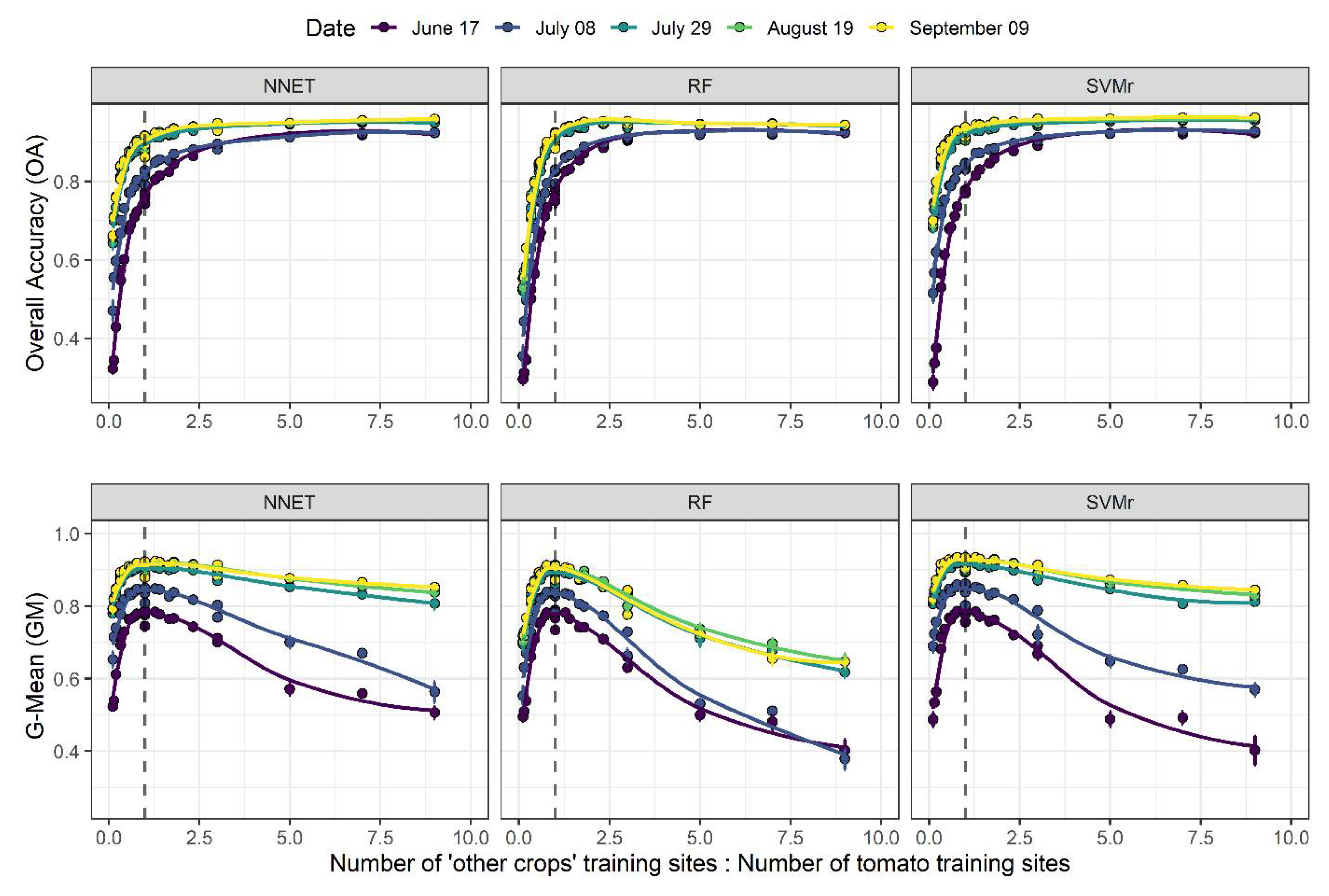
3.1. Simulation Results

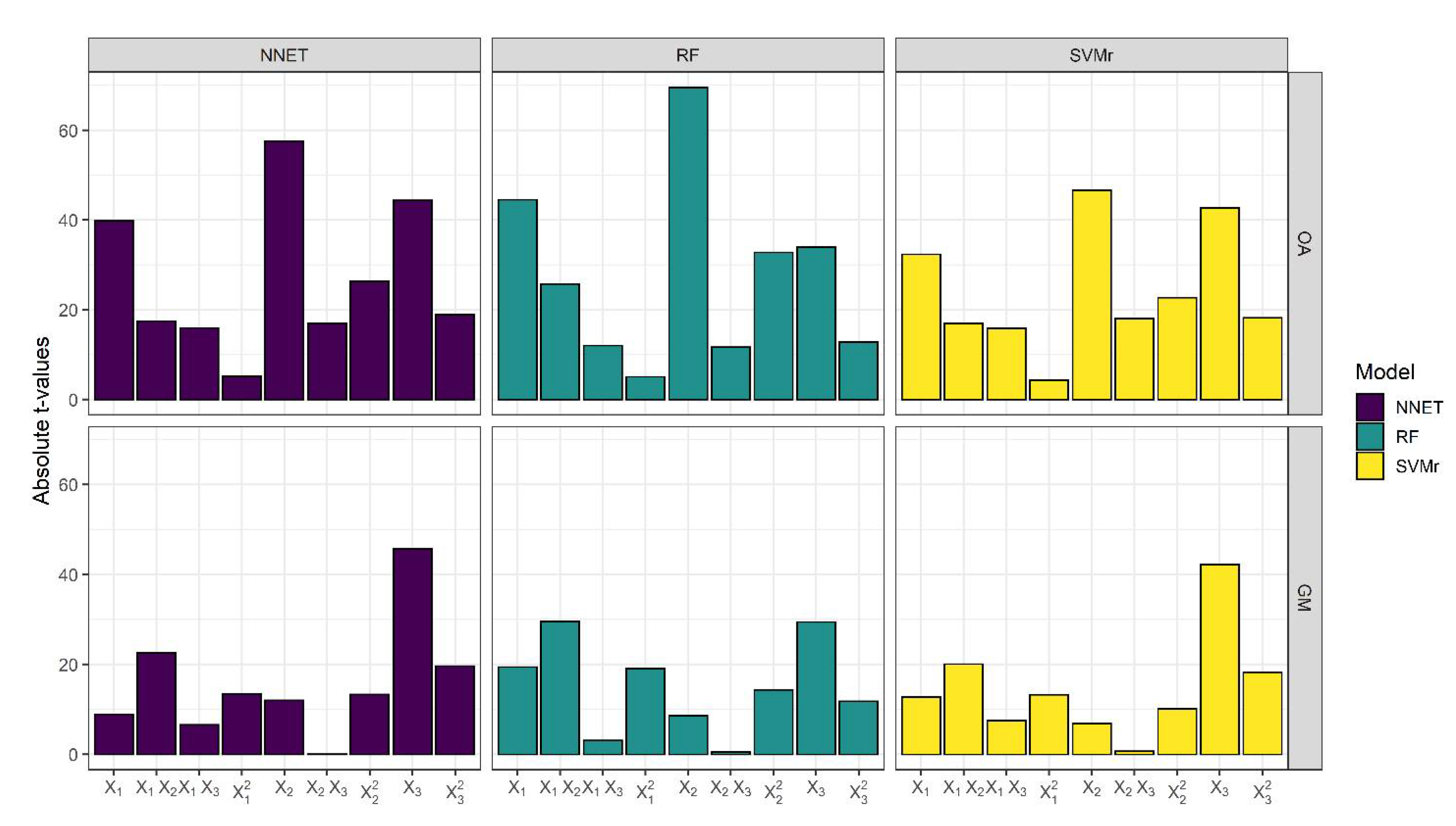
Figure 3 and Figure 4 display the evolution of OA and GM, respectively, as a function of the numerosity of tomato and ‘other crops’ training sites, for each of the three algorithms and for each lead time. In general, OA increases with the number of training sites and as the growing season progresses. At the beginning of the growing season (i.e., 17 June), OA increases the most when the number of ‘other crops’ training sites increases from low starting values, and this increment is even more important at high numbers of tomato training sites (e.g., 900). In addition, GM also increases with the increasing number of ‘other crops’ training sites, but only when the number of tomato training sites is high enough. When the number of tomato training sites is low (e.g., 100), the increment of ‘other crops’ training sites leads to a lowering of GM accuracy (Figure 4). This shows well that GM accuracy is strongly linked with the proportionality between the two classes. A reduction in performance is less evident as the growing season progresses and with the NNET and SVMr algorithms. This result is particularly evident in Figure 5, where the highest G-Mean performance is obtained when the training dataset has a ratio close to 1:1 between the majority and minority classes. The importance of the ratio of majority to minority class declines as the season progresses, and especially for the RF algorithm, which shows a more pronounced decline in performance as the ratio of the number of training sites to other crops to the number of tomato training sites increases above 1.

3.2. RSM Models

Multiple regression analysis using response surface methodology (RSM) was implemented to model the crop classification performance as a function of the three selected variables. The analysis was performed separately for both response variables (OA and GM) and for all three selected ML classifiers (SVMr, RF, and NNET).

The results of the analysis of variance (ANOVA) for the quadratic model for both response variables (OA and GM) and for all three ML classifiers (SVMr, RF, and NNET) are reported in Tables S1–S6. Linear, quadratic, and interaction terms were all highly statistically significant (p ≤ 0.001). The regression coefficient for linear terms X₁, X₂, and X₃ were highly significant (p ≤ 0.001) for both response variables and all ML classifiers. Most of the interactions of each linear term were also highly significant (p ≤ 0.001) for both response variables (Tables S7–S9). The only exception was the interaction between X₂ and X₃ for response variable GM that was not significant for all ML classifiers. Analysing the absolute t-value of the regression coefficients for the response variable GM (Tables S7–S9; Figure 6), it was observed that the linear term X₃ (lead time) was the most important independent variable in the GM maximization, followed by the interaction term X₁X₂ (number of tomato training sites and number of ‘other crops’ training sites, respectively). On the contrary, OA was mainly influenced by X₂ followed by X₃ (lead time) when SVMr and NNET were applied and by X₁ when RF was applied. The quadratic equation that best fit the data and the goodness of fit (R² and Adj. R²) is reported in

Table 5. Best fit of the quadratic equation for each classifier and each response variable. The independent variables X₁, X₂, and X₃ are the coded values for the number of tomato training sites, the number of ‘other crops’ training sites, and lead time.

ML Classifier	Response Variable	Equation	R2	Adj. R2
SVMr	OA	0.914 − 0.034X1 + 0.049X2 + 0.045X3 + 0.012X1X2 + 0.011X1X3 − 0.013X2X3 + 0.003X12 − 0.020X22 − 0.016X32	0.917	0.916
	GM	0.924 + 0.016X1 + 0.008X2 + 0.053X3 + 0.018X1X2 − 0.006X1X3 − 0.0006X2X3 − 0.014X12 − 0.010X22 − 0.019X32	0.833	0.830
RF	OA	0.884 − 0.047X1 + 0.074X2 + 0.036X3 + 0.019X1X2 + 0.009X1X3 − 0.008X2X3 + 0.004X12 − 0.029X22 − 0.011X32	0.943	0.9420
	GM	0.891 + 0.027X1 + 0.012X2 + 0.041X3 + 0.029X1X2 − 0.003X1X3 − 0.0005X2X3 − 0.022X12 − 0.017X22 − 0.014X32	0.826	0.823
NNET	OA	0.892 − 0.036X1 + 0.052X2 + 0.040X3 + 0.011X1 X2 + 0.010X1 X3 − 0.011X2X3 + 0.0039X12 − 0.020X22 − 0.014X32	0.935	0.934
	GM	0.911 + 0.009X1 + 0.012X2 + 0.047X3 + 0.016X1X2 − 0.004 X1X3 − 0.00002X2X3 − 0.011X12 − 0.011X22 − 0.017X32	0.854	0.852

. The R² and Adj. R² values for all responses are close to 1, showing the reliability and the strength of the relationship between the independent variable and the response. The Adj. R² values for GM were 0.830, 0.823, and 0.852 for SVMr, RF, and NNET, respectively. Higher adjusted R² values were observed for OA than for GM for each ML classifier: 0.916, 0.942, and 0.938 (SVMr, RF, and NNET, respectively). Hence, the multiple regression model was significant and adequately described response variables.

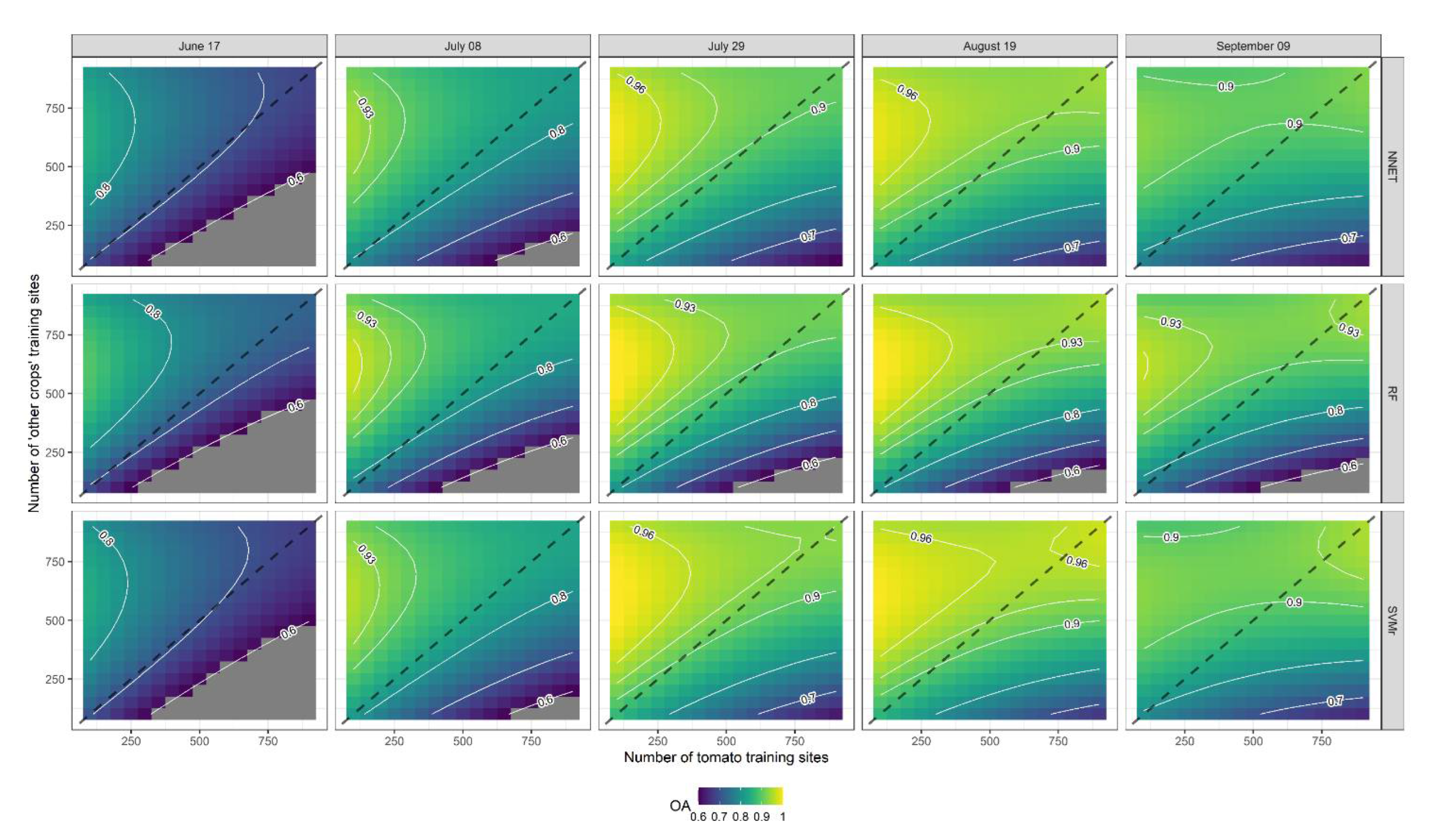
3.3. Effect of Training Set Size and Lead Time

Response contour plots of GM for each ML classifier (SVMr, NNET and RF) at each level of lead time (DOY 168, 189, 210, 231, and 252) are presented in Figure 7. In general, GM increases with the number of training sites, and as the season progresses until DOY 231 (19 August), while performance decreases on the subsequent date (DOY 252, 9 September). The GM response variable exhibited similar trends for all ML classifiers. The highest GM was observed near the 1:1 line when the number of training sites of tomato and ‘other crops’ were similar. In more detail, SVMr performed as the best ML classifier, achieving high levels of accuracy with a smaller number of training sites and a shorter lead time than the other two ML classifiers. It can be observed from OA contour plots (Figure 8) that SVMr achieved higher levels of accuracy with a shorter lead time than the other two algorithms (RF and NNET). However, the trend of OA as a response to the number of tomato and ‘other crops’ training sites is very different from that observed for GM. As observed from the analysis of the t-value in Figure 6, the number of ‘other crops’ training sites is one of the independent variables affecting the response variable (OA).

3.4. Optimization Using RSM

The independent variables X₁, X₂, and X₃, were optimized for both response variables (OA and GM) and all ML classifiers by solving the quadratic regression equation.

Table 6. Best condition for Overall Accuracy (OA) and G-Mean (GM) as a function of the number of tomato training sites (X₁), the number of other crop training sites (X₂), and the lead time (X₃).

ML Classifier	Response Variable	Y	X1	X2	X3
SVMr	OA	0.952	660	710	236
	GM	0.970	721	756	234
RF	OA	0.938	684	769	239
	GM	0.951	832	854	236
NNET	OA	0.931	720	749	237
	GM	0.953	702	749	235

reports the conditions for which the response variables and the three ML classifiers are maximized. The best combination of independent variables is slightly different for each algorithm. In general, all ML classifiers reach their maximum accuracy at the DOY 230–240 interval (18–28 August). At this interval of lead time, SVMr achieves the highest performance values, both in terms of OA and GM (0.95 and 0.97, respectively), with a combination of 660 and 721 of the number of tomato training sites and 710 and 756 of the number of ‘other crops’ training sites, respectively, for OA and GM.

4. Discussion

This study evaluates how tomato crop mapping accuracy is affected by the lead time and by the training set size, namely the number of ‘other crops’ training sites (majority class) and the number of tomato training sites (minority class). A CCRD and an RSM were applied to jointly analyse these effects and to fit them with a quadratic model. The analysis was performed separately for both response variables (OA and GM) and for all the three selected ML classifiers (SVMr, RF, and NNET). In general, the results confirmed that the characteristics of the training set (e.g., proportions between classes, size, number of classes) have a greater impact on performance than the choice of ML classifier [16,17,51].

4.1. Effect of Lead Time

The absolute t-values of the regression coefficients of these models enabled the importance of the three independent variables to be analysed. In particular, it was observed that the lead time (X₃) had the highest effect on the performance of crop classification for both evaluation metrics (OA and GM) and all three ML classifiers (SVMr, RF, and NNET). In mid-June (DOY 168), both evaluation metrics had the lowest values and then progressively increased during the growing season (Figure 3 and Figure 4). Low levels of early-season accuracy were also obtained in previous work and were attributed to the high similarity of the spectral responses of the crops to be classified [14,52]. When crops reach maturation, they instead develop distinctive properties, providing ML classifiers with more information, allowing for a more efficient discrimination between crops. In this way, the performances increase dramatically, reaching the maximum of their accuracy when the differences between vegetation indices are the most marked (i.e., mid-August, DOY 231).

In addition, for example, soybeans start their senescence at beginning of August, making them easily distinguishable from processing tomato. With the advancement of the season (i.e., 9 September, DOY 252), there is a general decline in performance (OA and GM) for all three ML classifiers, likely due to the sudden removal of biomass and to the scalarity of harvest dates for tomato [52,53]. In fact, the number of hectares harvested in tomatoes begins to be significant (approximately 50% of the areas) causing substantial intraclass variability, which results in reduced performance in tomato mapping. Similar results were reported by Azar and colleagues [14], who studied the trend of OA over time in a study area very close to the one used in the present work (Lombardy, Northern Italy). They observed that OA increased by 14–20% from the beginning of the season (13 May) to the 25 July, when it reached a plateau, and then decreased up to the end of the season (12 December).

4.2. Effect of Training Set Size

The second most important variable in modelling the GM response variable after the lead time (X₃) for all classifiers was the interaction between X₁ and X₂ (number of tomato training sites and number of ‘other crops’ training sites, respectively). This result is consistent with what the authors of [51] reported, that the algorithms evaluated were more sensitive to the proportion between classes rather than to the size of the training dataset. In the present work, GM maximization was achieved when the number of training sites of tomato and ‘other crops’ were balanced (1:1 ratio). This contrasts with reports from other studies, in which the authors argue that a 1:1 ratio between the two classes does not optimize accuracy unless this 1:1 ratio approaches the actual proportion of the observed territory [22,51,54]. However, the optimal proportion of the training set is often strongly influenced by the distance in feature space between the classes analysed [15], the evaluation metric one attempts to optimize, and the classes considered within the classification. In general, in this study, GM increased as the overall size of the dataset increased, consistently with what was reported in other studies [23,55]. Nevertheless, when extreme combinations of the number of training sites of tomato or ‘other crops’ were employed, even with only one of the two classes having few training sites (e.g., 100 training sites of tomato and 900 training sites of ‘other crops’ or vice versa), low levels of GM were achieved. This is due to the algorithm performing better when trained to correctly classify the most abundant class (either tomato or ‘other crops’) with a high number of training sites in the training set, reducing errors in this sense and maximizing sensitivity (or specificity). On the other hand, a ratio close to 1:1 balance sensitivity and sensibility, simultaneously, enables a high GM to be reached. Furthermore, the OA response variable (evaluation metric) showed a strong dependence on the ‘other crops’ class (majority class) [51]. This is due to the high disproportion between tomato and other crop fields within the test dataset (1:15). The high imbalance entails those high levels of OA are achieved already with a low number of tomato training sites. However, as the number of tomato training sites increases, classifiers will also be able to classify tomato fields correctly, and thus OA will increase as well.

4.3. Tomato Crop Mapping Optimization

Solving the quadratic model describing the response surface as a function of X₁, X₂, and X₃ enabled the identification of stationary points (local maxima) for each classifier and for both evaluation metrics (Table 6). SVMr was the best ML classifier, confirming previous studies [26,51]. SVMr achieved higher OA and GM (0.95 and 0.97, respectively) using fewer training sites than the other ML classifiers (RF and NNET). According to [56], the high performance of SVMr can be attributed to SVMr being less sensitive to intraclass variation. This, in turn, can be attributed to the fact that SVMr only needs a subsample for the computation of support vectors to define the separation hyperplane. Therefore, only the samples that lie on the edge of the class distribution in the feature space are needed to achieve high levels of crop mapping accuracy [56]. In addition, SVMr—as can be seen from the contour plot in Figure 3—despite reaching its peak performance at 660 (X₁) and 710 (X₂) for OA and 721 (X₁) and 756 (X₂) for GM, reaches levels above 0.93 already with much lower numbers of training sites. In general, all classifiers showed the highest levels of accuracy between DOY 230–240, the peak performance having been reached in mid-August (i.e., DOY 231), i.e., approximately 120–140 days after the nominal start of the growing season, when the maximum vegetation indices are exceeded [57,58].

These results are supposed to be due to the fact that crops reach their maximum difference in vegetation index trends in mid-August, while low accuracies in tomato classification are due to vegetation index trends of the crops being in overlap (at the start of the growing season) and influenced by crop senescence, biomass removal, and tomato harvest (at the end of the growing season).

5. Conclusions

This study analysed the combined effects of training set size and lead time on the performance of three ML classifiers (RF, SVMr, and NNET) in tomato classification, by identifying the optimal trade-off for each of the classifiers. The performance exceeded 0.95 for both evaluation metrics analysed (OA and GM), showing that tomato mapping provides reliable information that enables a range of field information such as phenology, health status, and production potential to be derived to better optimize the management of the tomato supply chain. The results show that lead time is the main factor for maximizing classification performance according to both evaluation metrics analysed. The second most important factor (for GM) is the ratio of the number of tomato and ‘other crops’ training sites, which maximizes the classification performance when close to 1. These findings provide useful information for building and planning the tomato classification workflow, and highlight the need to update the tomato crop mapping up to DOY 230–240 to achieve maximum performance and to train the classifiers with a balanced number of training sites between the two classes (tomato and ‘other crops’ classes). In addition, the use of SVMr is recommended as this classifier reached its peak performance sooner in the season (low lead time) than the other two. SVMr also needed fewer training sites, allowing for reduced cost and time for ground truth collection through field expeditions.

References

1. Gallego, F.J.; Kussul, N.; Skakun, S.; Kravchenko, O.; Shelestov, A.; Kussul, O. Efficiency Assessment of Using Satellite Data for Crop Area Estimation in Ukraine. Int. J. Appl. Earth Obs. Geoinf. 2014, 29, 22–30. [Google Scholar] [CrossRef]
2. Craig, M.; Atkinson, D. A Literature Review of Crop Area Estimation; FAO Publication: Rome, Italy, 2013. [Google Scholar]
3. Miranda, J.; Ponce, P.; Molina, A.; Wright, P. Sensing, Smart and Sustainable Technologies for Agri-Food 4.0. Comput. Ind. 2019, 108, 21–36. [Google Scholar] [CrossRef]
4. Lezoche, M.; Hernandez, J.E.; Alemany Díaz, M.D.M.E.; Panetto, H.; Kacprzyk, J. Agri-Food 4.0: A Survey of the Supply Chains and Technologies for the Future Agriculture. Comput. Ind. 2020, 117, 103187. [Google Scholar] [CrossRef]
5. Immitzer, M.; Vuolo, F.; Atzberger, C. First Experience with Sentinel-2 Data for Crop and Tree Species Classifications in Central Europe. Remote Sens. 2016, 8, 166. [Google Scholar] [CrossRef]
6. Olofsson, P.; Foody, G.M.; Herold, M.; Stehman, S.V.; Woodcock, C.E.; Wulder, M.A. Good Practices for Estimating Area and Assessing Accuracy of Land Change. Remote Sens. Environ. 2014, 148, 42–57. [Google Scholar] [CrossRef]
7. Kavats, O.; Khramov, D.; Sergieieva, K.; Vasyliev, V. Monitoring of Sugarcane Harvest in Brazil Based on Optical and {SAR} Data. Remote Sens. 2020, 12, 4080. [Google Scholar] [CrossRef]
8. Kavats, O.; Khramov, D.; Sergieieva, K.; Vasyliev, V. Monitoring Harvesting by Time Series of Sentinel-1 {SAR} Data. Remote Sens. 2019, 11, 2496. [Google Scholar] [CrossRef]
9. Gao, F.; Zhang, X. Mapping Crop Phenology in Near Real-Time Using Satellite Remote Sensing: Challenges and Opportunities. J. Remote Sens. 2021, 2021, 1–14. [Google Scholar] [CrossRef]
10. Meroni, M.; d’Andrimont, R.; Vrieling, A.; Fasbender, D.; Lemoine, G.; Rembold, F.; Seguini, L.; Verhegghen, A. Comparing Land Surface Phenology of Major European Crops as Derived from {SAR} and Multispectral Data of Sentinel-1 and -2. Remote Sens. Environ. 2021, 253, 112232. [Google Scholar] [CrossRef]
11. Kamir, E.; Waldner, F.; Hochman, Z. Estimating Wheat Yields in Australia Using Climate Records, Satellite Image Time Series and Machine Learning Methods. ISPRS J. Photogramm. Remote Sens. 2020, 160, 124–135. [Google Scholar] [CrossRef]
12. Meroni, M.; Waldner, F.; Seguini, L.; Kerdiles, H.; Rembold, F. Yield Forecasting with Machine Learning and Small Data: What Gains for Grains? Agric. For. Meteorol. 2021, 308–309, 108555. [Google Scholar] [CrossRef]
13. FAO; IFAD; IMF; OECD; UNCTAD; WFP; World Bank; WTO; IFPRI; United Nations High Level Task Force on Global Food and Nutrition. Price Volatility in Food and Agricultural Markets: Policy Responses; World Bank: Washington, DC, USA, 2011. [Google Scholar]
14. Azar, R.; Villa, P.; Stroppiana, D.; Crema, A.; Boschetti, M.; Brivio, P.A. Assessing In-Season Crop Classification Performance Using Satellite Data: A Test Case in Northern Italy. Eur. J. Remote Sens. 2016, 49, 361–380. [Google Scholar] [CrossRef]
15. Foody, G.M.; Mathur, A.; Sanchez-Hernandez, C.; Boyd, D.S. Training Set Size Requirements for the Classification of a Specific Class. Remote Sens. Environ. 2006, 104, 1–14. [Google Scholar] [CrossRef]
16. Ramezan, C.A.; Warner, T.A.; Maxwell, A.E.; Price, B.S. Effects of Training Set Size on Supervised Machine-Learning Land-Cover Classification of Large-Area High-Resolution Remotely Sensed Data. Remote Sens. 2021, 13, 368. [Google Scholar] [CrossRef]
17. Foody, G.M.; Arora, M.K. An Evaluation of Some Factors Affecting the Accuracy of Classification by an Artificial Neural Network. Int. J. Remote Sens. 1997, 18, 799–810. [Google Scholar] [CrossRef]
18. Foody, G.M.; Mathur, A. A Relative Evaluation of Multiclass Image Classification by Support Vector Machines. IEEE Trans. Geosci. Remote Sens. 2004, 42, 1335–1343. [Google Scholar] [CrossRef]
19. Congalton, R.G.; Green, K. Assessing the Accuracy of Remotely Sensed Data: Principles and Practices, 2nd ed.; CRC Press: Boca Raton, FL, USA, 2008. [Google Scholar]
20. Foody, G.M. Status of Land Cover Classification Accuracy Assessment. Remote Sens. Environ. 2002, 80, 185–201. [Google Scholar] [CrossRef]
21. Foody, G.M.; McCulloch, M.B.; Yates, W.B. The Effect of Training Set Size and Composition on Artificial Neural Network Classification. Int. J. Remote Sens 1995, 16, 1707–1723. [Google Scholar] [CrossRef]
22. Millard, K.; Richardson, M. On the Importance of Training Data Sample Selection in Random Forest Image Classification: A Case Study in Peatland Ecosystem Mapping. Remote Sens. 2015, 7, 8489–8515. [Google Scholar] [CrossRef]
23. Qian, Y.; Zhou, W.; Yan, J.; Li, W.; Han, L. Comparing Machine Learning Classifiers for Object-Based Land Cover Classification Using Very High Resolution Imagery. Remote Sens 2015, 7, 153–168. [Google Scholar] [CrossRef]
24. Heydari, S.S.; Mountrakis, G. Effect of Classifier Selection, Reference Sample Size, Reference Class Distribution and Scene Heterogeneity in per-Pixel Classification Accuracy Using 26 Landsat Sites. Remote Sens. Environ. 2018, 204, 648–658. [Google Scholar] [CrossRef]
25. Noi, P.T.; Kappas, M. Comparison of Random Forest, k-Nearest Neighbor, and Support Vector Machine Classifiers for Land Cover Classification Using Sentinel-2 Imagery. Sensors 2018, 18, 18. [Google Scholar]
26. Myburgh, G.; van Niekerk, A. Effect of Feature Dimensionality on Object-Based Land Cover Classification: A Comparison of Three Classifiers. South Afr. J. Geomat. 2013, 2, 13–27. [Google Scholar]
27. Dean, A.; Voss, D.; Draguljić, D. Response Surface Methodology. In Springer Texts in Statistics; Springer International Publishing: Cham, Switzerland, 2017; pp. 565–614. [Google Scholar]
28. Peel, M.C.; Finlayson, B.L.; McMahon, T.A. Updated World Map of the Köppen-Geiger Climate Classification. Hydrol. Earth Syst. Sci. Discuss. 2007, 4, 439–473. [Google Scholar] [CrossRef]
29. Drusch, M.; del Bello, U.; Carlier, S.; Colin, O.; Fernandez, V.; Gascon, F.; Hoersch, B.; Isola, C.; Laberinti, P.; Martimort, P.; et al. Sentinel-2: ESA’s Optical High-Resolution Mission for GMES Operational Services. Remote Sens. Environ. 2012, 120, 25–36. [Google Scholar] [CrossRef]
30. THEIA Value-Adding Products and Algorithms for Land Surfaces. Available online: https://www.theia-land.fr/ (accessed on 20 January 2021).
31. Lonjou, V.; Desjardins, C.; Hagolle, O.; Petrucci, B.; Tremas, T.; Dejus, M.; Makarau, A.; Auer, S. MACCS-ATCOR Joint Algorithm (MAJA). In Proceedings of the Remote Sensing of Clouds and the Atmosphere XXI; Comerón, A., Kassianov, E.I., Schäfer, K., Eds.; SPIE: Washington, DC, USA, 2016. [Google Scholar]
32. GDAL Documentation. Available online: www.gdal.org (accessed on 20 December 2021).
33. Griffiths, P.; Nendel, C.; Hostert, P. Intra-Annual Reflectance Composites from Sentinel-2 and Landsat for National-Scale Crop and Land Cover Mapping. Remote Sens. Environ. 2019, 220, 135–151. [Google Scholar] [CrossRef]
34. Rouse, J.W.; Hass, R.H.; Schell, J.A.; Deering, D.W. Monitoring Vegetation Systems in the Great Plains with ERTS. NASA ERTS Symp. 1973, 1, 309–313. [Google Scholar]
35. Gitelson, A.; Merzlyak, M.N. Quantitative Estimation of Chlorophyll-a Using Reflectance Spectra: Experiments with Autumn Chestnut and Maple Leaves. J. Photochem. Photobiol. B 1994, 22, 247–252. [Google Scholar] [CrossRef]
36. Gao, B.-C. NDWI—A Normalized Difference Water Index for Remote Sensing of Vegetation Liquid Water from Space. Remote Sens. Environ. 1996, 58, 257–266. [Google Scholar] [CrossRef]
37. Louhaichi, M.; Borman, M.M.; Johnson, D.E. Spatially Located Platform and Aerial Photography for Documentation of Grazing Impacts on Wheat. Geocarto Int. 2001, 16, 65–70. [Google Scholar] [CrossRef]
38. Vincini, M.; Frazzi, E.; D’Alessio, P. A Broad-Band Leaf Chlorophyll Vegetation Index at the Canopy Scale. Precis. Agric. 2008, 9, 303–319. [Google Scholar] [CrossRef]
39. Gitelson, A.A. Wide Dynamic Range Vegetation Index for Remote Quantification of Biophysical Characteristics of Vegetation. J. Plant Physiol. 2004, 161, 165–173. [Google Scholar] [CrossRef] [PubMed]
40. Lenth, R.V. Response-Surface Methods InR, Usingrsm. J. Stat. Softw. 2009, 32, 1–17. [Google Scholar] [CrossRef] [Green Version]
41. Breiman, L. Random Forests. Mach. Learn. 2001, 45, 5–32. [Google Scholar] [CrossRef]
42. Murtagh, F. Multilayer Perceptrons for Classification and Regression. Neurocomputing 1991, 2, 183–197. [Google Scholar] [CrossRef]
43. Vapnik, V. The Support Vector Method of Function Estimation. In Nonlinear Modeling; Springer US: Boston, MA, USA, 1998; pp. 55–85. [Google Scholar]
44. Kuhn, M.; Johnson, K. Applied Predictive Modeling; Springer: New York, NY, USA, 2019. [Google Scholar]
45. Arlot, S.; Celisse, A. A Survey of Cross-Validation Procedures for Model Selection. Stat. Surv. 2010, 4, 40–79. [Google Scholar] [CrossRef]
46. Ramezan, C.A.; Warner, T.A.; Maxwell, A.E. Evaluation of Sampling and Cross-Validation Tuning Strategies for Regional-Scale Machine Learning Classification. Remote Sens. 2019, 11, 185. [Google Scholar] [CrossRef]
47. Picard, R.R.; Cook, R.D. Cross-Validation of Regression Models. J. Am. Stat. Assoc. 1984, 79, 575. [Google Scholar] [CrossRef]
48. He, H.; Garcia, E.A. Learning from Imbalanced Data. IEEE Trans. Knowl. Data Eng. 2009, 21, 1263–1284. [Google Scholar]
49. Waldner, F.; Chen, Y.; Lawes, R.; Hochman, Z. Needle in a Haystack: Mapping Rare and Infrequent Crops Using Satellite Imagery and Data Balancing Methods. Remote Sens. Environ. 2019, 233, 111375. [Google Scholar] [CrossRef]
50. Fowler, J.; Waldner, F.; Hochman, Z. All Pixels Are Useful, but Some Are More Useful: Efficient in Situ Data Collection for Crop-Type Mapping Using Sequential Exploration Methods. ITC J. 2020, 91, 102114. [Google Scholar] [CrossRef]
51. Waldner, F.; Jacques, D.C.; Löw, F. The Impact of Training Class Proportions on Binary Cropland Classification. Remote Sens. Lett. 2017, 8, 1122–1131. [Google Scholar] [CrossRef]
52. Maponya, M.G.; van Niekerk, A.; Mashimbye, Z.E. Pre-Harvest Classification of Crop Types Using a Sentinel-2 Time-Series and Machine Learning. Comput. Electron. Agric. 2020, 169, 105164. [Google Scholar] [CrossRef]
53. Veloso, A.; Mermoz, S.; Bouvet, A.; le Toan, T.; Planells, M.; Dejoux, J.F.; Ceschia, E. Understanding the Temporal Behavior of Crops Using Sentinel-1 and Sentinel-2-like Data for Agricultural Applications. Remote Sens. Environ. 2017, 199, 415–426. [Google Scholar] [CrossRef]
54. Zhu, Z.; Gallant, A.L.; Woodcock, C.E.; Pengra, B.; Olofsson, P.; Loveland, T.R.; Jin, S.; Dahal, D.; Yang, L.; Auch, R.F. Optimizing Selection of Training and Auxiliary Data for Operational Land Cover Classification for the LCMAP Initiative. ISPRS J. Photogramm. Remote Sens. 2016, 122, 206–221. [Google Scholar] [CrossRef]
55. Shang, M.; Wang, S.-X.; Zhou, Y.; Du, C. Effects of Training Samples and Classifiers on Classification of Landsat-8 Imagery. J. Ind. Soc. Remote Sens. 2018, 46, 1333–1340. [Google Scholar] [CrossRef]
56. Zheng, B.; Myint, S.W.; Thenkabail, P.S.; Aggarwal, R.M. A Support Vector Machine to Identify Irrigated Crop Types Using Time-Series Landsat NDVI Data. ITC J. 2015, 34, 103–112. [Google Scholar] [CrossRef]
57. Van Niel, T.G.; McVicar, T.R. Determining Temporal Windows for Crop Discrimination with Remote Sensing: A Case Study in South-Eastern Australia. Comput. Electron. Agric. 2004, 45, 91–108. [Google Scholar] [CrossRef]
58. Matton, N.; Canto, G.; Waldner, F.; Valero, S.; Morin, D.; Inglada, J.; Arias, M.; Bontemps, S.; Koetz, B.; Defourny, P. An Automated Method for Annual Cropland Mapping along the Season for Various Globally-Distributed Agrosystems Using High Spatial and Temporal Resolution Time Series. Remote Sens. 2015, 7, 13208–13232. [Google Scholar] [CrossRef] [Green Version]
Figure 1. The study area was in the Emilia-Romagna region in the North of Italy (orange area, covered by Sentinel-2 tiles 32TNQ, 32TPQ, and 32TQQ).
Remotesensing 14 04540 g001
Figure 2. Temporal profiles based on the NDVI, NDRE, NDWI, GNDVI, CVI and greenWDRVI of the targeted crops during the growing season in the study area. The lines represent the average values of VIs, and the grey shadow represents the period between DOY 190 and 220.
Remotesensing 14 04540 g002
Figure 3. Overall Accuracy progress over the number of ‘other crops’ training sites at different number of tomato training sites and lead time.
Remotesensing 14 04540 g003
Figure 4. G-Mean progress over the number of ‘other crops’ training sites at different numbers of tomato training sites and lead time.
Remotesensing 14 04540 g004
Figure 5. Overall Accuracy and G-Mean progress over the ratio between the number of ‘other crops’ training sites and the number of tomato training sites at different lead time. The dotted line represents the 1:1 ratio.
Remotesensing 14 04540 g005
Figure 6. Absolute t-value of each regression coefficient retrieved by RSM models.
Remotesensing 14 04540 g006
Figure 7. Response contour plots for G-Mean (GM) as a function of the number of tomato training sites (X1) and the number of ‘other crops’ training sites (X2). The dashed line represents a 1:1 line between X1 and X2.
Remotesensing 14 04540 g007
Figure 8. Response contour plots for Overall Accuracy (OA) as a function of the number of tomato training sites (X1) and the number of other crop training sites (X2). The dashed line represents a 1:1 line between X1 and X2.
Remotesensing 14 04540 g008