
Satellite-Derived Bottom Depth for Optically Shallow Waters Based on Hydrolight Simulations
 , ,
, ,
Abstract
:
1. Introduction
2. Materials and Methods
2.1. ICESat-2 Data
2.1.1. Identification of Water Surface and Bottom Signals
2.1.2. Bathymetric Correction
2.2. Sentinel-2 Satellite Imagery
2.3. Extraction of Optically Shallow Waters
2.4. Radiative Transfer Simulations by the Hydrolight
3. Development of the Bottom Depth Retrieval Model
3.1. Generation of Simulated Datasets
3.2. Model Training and Evaluation
4. Results
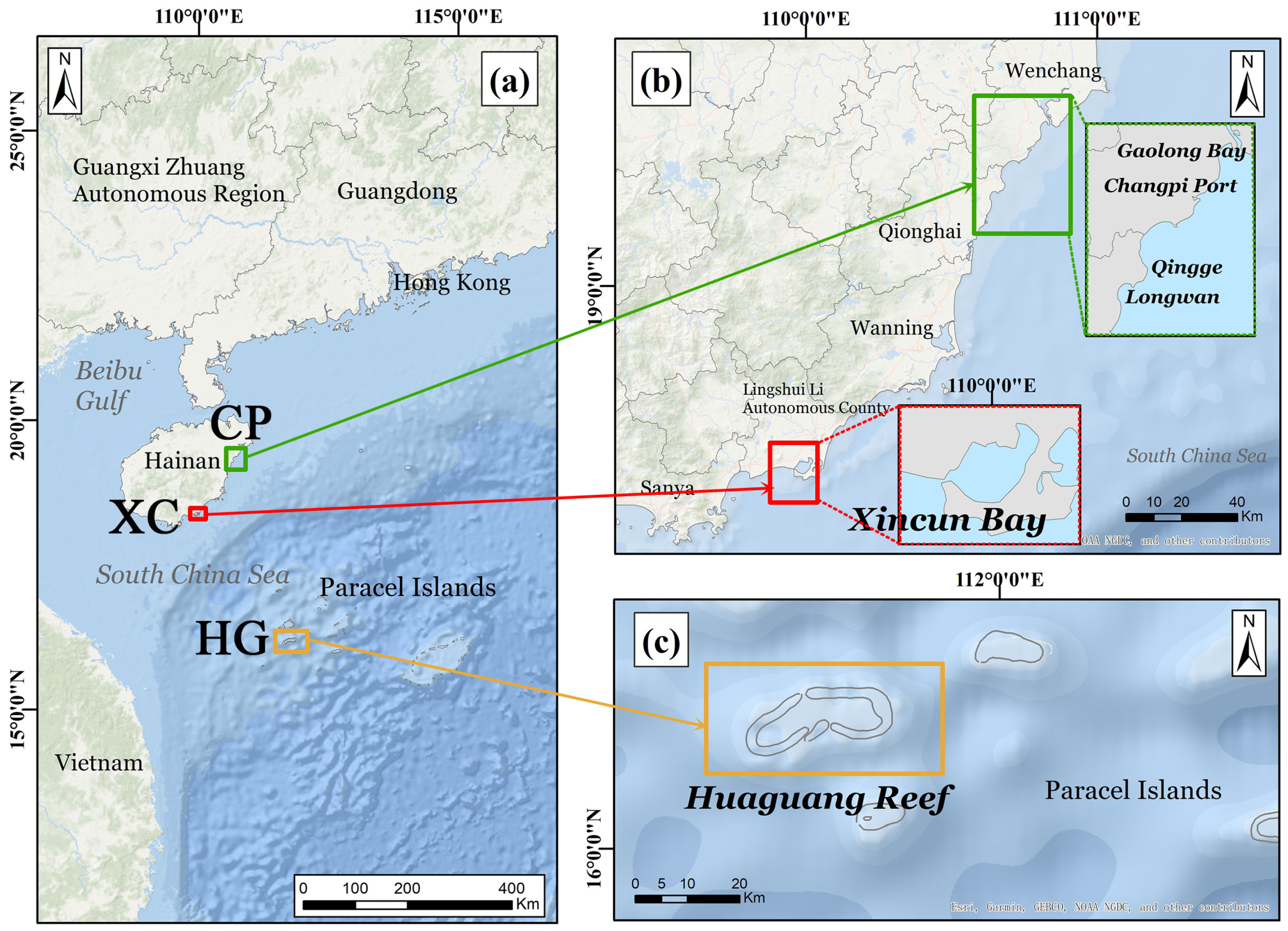
4.1. Validation Sites
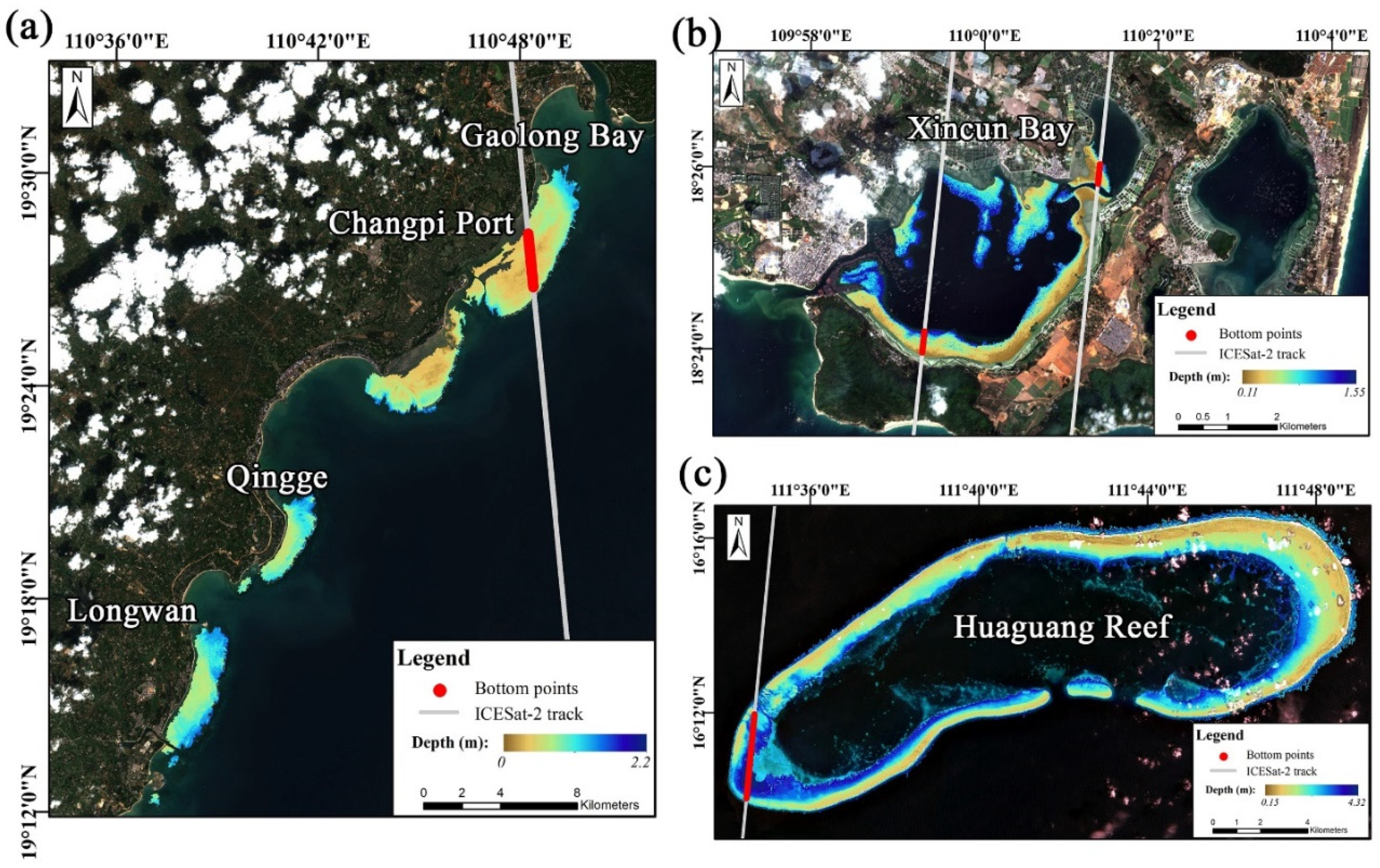
4.2. Bottom Depth Derived from Sentinel-2 Imagery
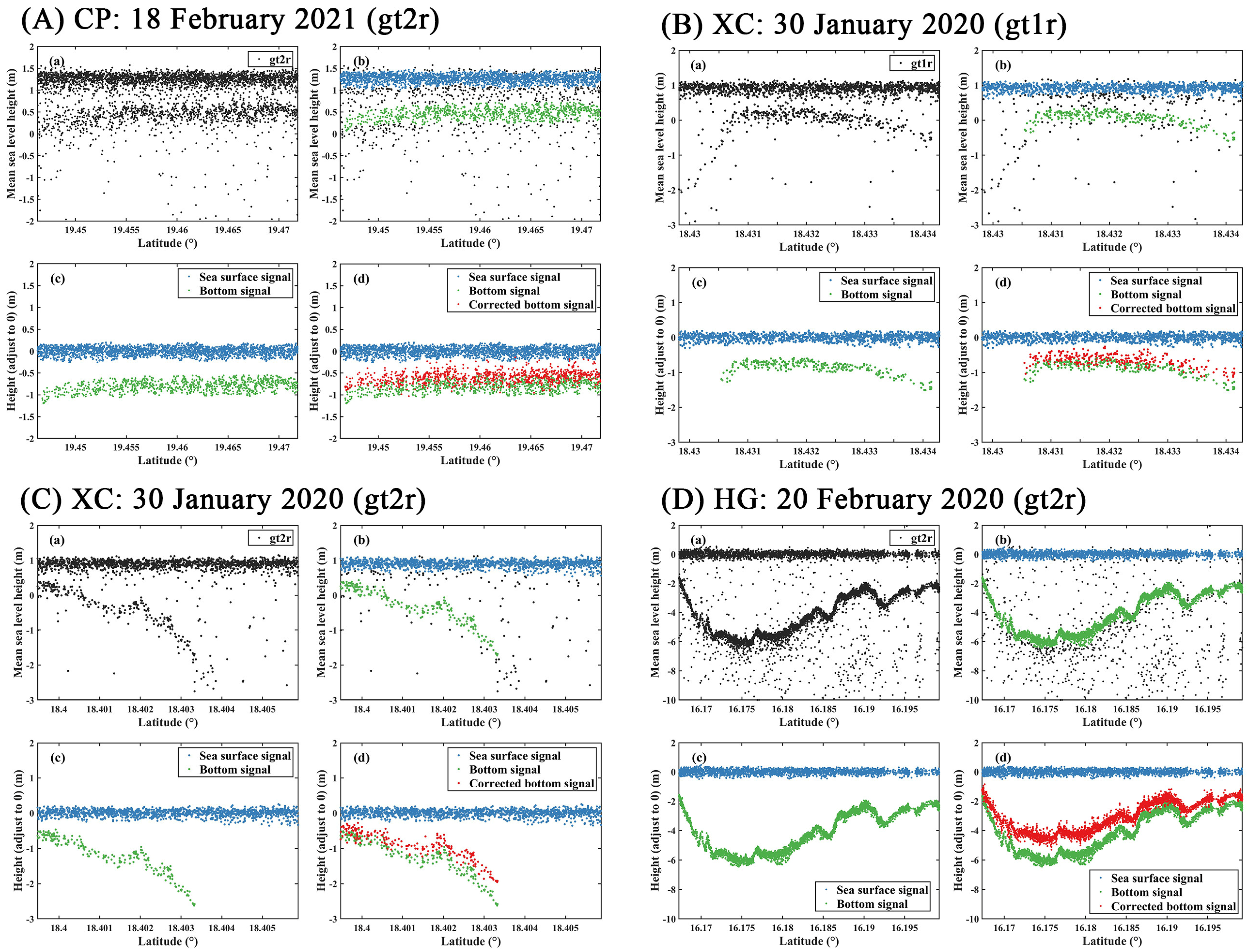
4.3. Bottom Depth Validation Based on ICESat-2 Along-Track Data
5. Discussion
6. Conclusions
Author Contributions
Funding
Data Availability Statement
Acknowledgments
Conflicts of Interest
References
- Eyre, B.D.; Ferguson, A.J.P.; Webb, A.; Maher, D.; Oakes, J.M. Metabolism of Different Benthic Habitats and Their Contribution to the Carbon Budget of a Shallow Oligotrophic Sub-Tropical Coastal System (Southern Moreton Bay, Australia). Biogeochemistry 2011, 102, 87–110. [Google Scholar] [CrossRef]
- Waycott, M.; Duarte, C.M.; Carruthers, T.J.B.; Orth, R.J.; Dennison, W.C.; Olyarnik, S.; Calladine, A.; Fourqurean, J.W.; Heck, K.L.; Hughes, A.R.; et al. Accelerating Loss of Seagrasses across the Globe Threatens Coastal Ecosystems. Proc. Natl. Acad. Sci. USA 2009, 106, 12377–12381. [Google Scholar] [CrossRef] [PubMed]
- Newton, A.; Icely, J.; Cristina, S.; Brito, A.; Cardoso, A.C.; Colijn, F.; Riva, S.D.; Gertz, F.; Hansen, J.W.; Holmer, M.; et al. An Overview of Ecological Status, Vulnerability and Future Perspectives of European Large Shallow, Semi-Enclosed Coastal Systems, Lagoons and Transitional Waters. Estuar. Coast. Shelf Sci. 2014, 140, 95–122. [Google Scholar] [CrossRef]
- Lyzenga, D.R.; Malinas, N.P.; Tanis, F.J. Multispectral Bathymetry Using a Simple Physically Based Algorithm. IEEE Trans. Geosci. Remote Sens. 2006, 44, 2251–2259. [Google Scholar] [CrossRef]
- Hedley, J.D.; Roelfsema, C.; Brando, V.; Giardino, C.; Kutser, T.; Phinn, S.; Mumby, P.J.; Barrilero, O.; Laporte, J.; Koetz, B. Coral Reef Applications of Sentinel-2: Coverage, Characteristics, Bathymetry and Benthic Mapping with Comparison to Landsat 8. Remote Sens. Environ. 2018, 216, 598–614. [Google Scholar] [CrossRef]
- Li, J.; Knapp, D.E.; Schill, S.R.; Roelfsema, C.; Phinn, S.; Silman, M.; Mascaro, J.; Asner, G.P. Adaptive Bathymetry Estimation for Shallow Coastal Waters Using Planet Dove Satellites. Remote Sens. Environ. 2019, 232, 111302. [Google Scholar] [CrossRef]
- Kutser, T. Remote Sensing of Shallow Waters—A 50 Year Retrospective and Future Directions. Remote Sens. Environ. 2020, 18, 111619. [Google Scholar] [CrossRef]
- Lyzenga, D.R. Passive Remote Sensing Techniques for Mapping Water Depth and Bottom Features. Appl. Opt. 1978, 17, 379. [Google Scholar] [CrossRef]
- Stumpf, R.P.; Holderied, K.; Sinclair, M. Determination of Water Depth with High-Resolution Satellite Imagery over Variable Bottom Types. Limnol. Oceanogr. 2003, 48, 547–556. [Google Scholar] [CrossRef]
- Caballero, I.; Stumpf, R.P. Retrieval of Nearshore Bathymetry from Sentinel-2A and 2B Satellites in South Florida Coastal Waters. Estuar. Coast. Shelf Sci. 2019, 226, 106277. [Google Scholar] [CrossRef]
- Cahalane, C.; Magee, A.; Monteys, X.; Casal, G.; Hanafin, J.; Harris, P. A Comparison of Landsat 8, RapidEye and Pleiades Products for Improving Empirical Predictions of Satellite-Derived Bathymetry. Remote Sens. Environ. 2019, 233, 111414. [Google Scholar] [CrossRef] [PubMed]
- Dekker, A.G.; Phinn, S.R.; Anstee, J.; Bissett, P.; Brando, V.E.; Casey, B.; Fearns, P.; Hedley, J.; Klonowski, W.; Lee, Z.P.; et al. Intercomparison of Shallow Water Bathymetry, Hydro-Optics, and Benthos Mapping Techniques in Australian and Caribbean Coastal Environments. Limnol. Oceanogr. Methods 2011, 9, 396–425. [Google Scholar] [CrossRef]
- Lee, Z.; Carder, K.L.; Mobley, C.D.; Steward, R.G.; Patch, J.S. Hyperspectral Remote Sensing for Shallow Waters I A Semianalytical Model. Appl. Opt. 1998, 37, 6329. [Google Scholar] [CrossRef]
- Lee, Z.; Carder, K.L.; Mobley, C.D.; Steward, R.G.; Patch, J.S. Hyperspectral Remote Sensing for Shallow Waters: 2 Deriving Bottom Depths and Water Properties by Optimization. Appl. Opt. 1999, 38, 3831. [Google Scholar] [CrossRef] [PubMed]
- Lee, Z.; Carder, K.L.; Chen, R.F.; Peacock, T.G. Properties of the Water Column and Bottom Derived from Airborne Visible Infrared Imaging Spectrometer (AVIRIS) Data. J. Geophys. Res. Oceans 2001, 106, 11639–11651. [Google Scholar] [CrossRef]
- Mobley, C.D.; Sundman, L.K.; Davis, C.O.; Bowles, J.H.; Downes, T.V.; Leathers, R.A.; Montes, M.J.; Bissett, W.P.; Kohler, D.D.R.; Reid, R.P.; et al. Interpretation of Hyperspectral Remote-Sensing Imagery by Spectrum Matching and Look-up Tables. Appl. Opt. 2005, 44, 3576. [Google Scholar] [CrossRef]
- Hu, L.; Liu, Z.; Liu, Z.; Hu, C.; He, M.-X. Mapping Bottom Depth and Albedo in Coastal Waters of the South China Sea Islands and Reefs Using Landsat TM and ETM+ Data. Int. J. Remote Sens. 2014, 35, 4156–4172. [Google Scholar] [CrossRef]
- Liu, S.; Wang, L.; Liu, H.; Su, H.; Li, X.; Zheng, W. Deriving Bathymetry from Optical Images with a Localized Neural Network Algorithm. IEEE Trans. Geosci. Remote Sens. 2018, 56, 5334–5342. [Google Scholar] [CrossRef]
- Lai, W.; Lee, Z.; Wang, J.; Wang, Y.; Garcia, R.; Zhang, H. A Portable Algorithm to Retrieve Bottom Depth of Optically Shallow Waters from Top-of-Atmosphere Measurements. J. Remote Sens. 2022, 2022, 9831947. [Google Scholar] [CrossRef]
- Manessa, M.D.M.; Setiawan, K.T.; Haidar, M.; Supriatna, S.; Pataropura, A.; Supardjo, A.H. Optimization of the Random Forest Algorithm for Multispectral Derived Bathymetry. Int. J. Geoinf. 2020, 16, 1–6. [Google Scholar]
- Breiman, L. Random Forests. Mach. Learn. 2001, 45, 5–32. [Google Scholar] [CrossRef] [Green Version]
- Manessa, M.D.M.; Kanno, A.; Sekine, M.; Haidar, M.; Yamamoto, K.; Imai, T.; Higuchi, T. Satellite-Derived Bathymetry Using Random Forest Algorithm and Worldview-2 Imagery. J. Geomat. Plan. 2016, 3, 10. [Google Scholar] [CrossRef]
- Sagawa, T.; Yamashita, Y.; Okumura, T.; Yamanokuchi, T. Satellite Derived Bathymetry Using Machine Learning and Multi-Temporal Satellite Images. Remote Sens. 2019, 11, 1155. [Google Scholar] [CrossRef]
- Babbel, B.J.; Parrish, C.E.; Magruder, L.A. ICESat-2 Elevation Retrievals in Support of Satellite-Derived Bathymetry for Global Science Applications. Geophys. Res. Lett. 2021, 48, e2020GL090629. [Google Scholar] [CrossRef]
- Ma, Y.; Xu, N.; Liu, Z.; Yang, B.; Yang, F.; Wang, X.H.; Li, S. Satellite-Derived Bathymetry Using the ICESat-2 Lidar and Sentinel-2 Imagery Datasets. Remote Sens. Environ. 2020, 250, 112047. [Google Scholar] [CrossRef]
- Thomas, N.; Pertiwi, A.P.; Traganos, D.; Lagomasino, D.; Poursanidis, D.; Moreno, S.; Fatoyinbo, L. Space-Borne Cloud-Native Satellite-Derived Bathymetry (SDB) Models Using ICESat-2 And Sentinel-2. Geophys. Res. Lett. 2021, 48, e2020GL092170. [Google Scholar] [CrossRef]
- Mobley, C.D.; Sundman, L.K. Hydrolight 5 Ecolight 5 Technical Documentation; Sequoia Scientific, Inc.: Bellevue, WA, USA, 2008; p. 100. [Google Scholar]
- Mobley, C.D.; Sundman, L.K. Hydrolight 5 Ecolight 5 Users Guide; Sequoia Scientific, Inc.: Bellevue, WA, USA, 2008; p. 104. [Google Scholar]
- Parrish, C.E.; Magruder, L.A.; Neuenschwander, A.L.; Forfinski-Sarkozi, N.; Alonzo, M.; Jasinski, M. Validation of ICESat-2 ATLAS Bathymetry and Analysis of ATLAS’s Bathymetric Mapping Performance. Remote Sens. 2019, 11, 1634. [Google Scholar] [CrossRef]
- Coveney, S.; Monteys, X.; Hedley, J.D.; Castillo-Campo, Y.; Kelleher, B. ICESat-2 Marine Bathymetry: Extraction, Refraction Adjustment and Vertical Accuracy as a Function of Depth in Mid-Latitude Temperate Contexts. Remote Sens. 2021, 13, 4352. [Google Scholar] [CrossRef]
- Markus, T.; Neumann, T.; Martino, A.; Abdalati, W.; Brunt, K.; Csatho, B.; Farrell, S.; Fricker, H.; Gardner, A.; Harding, D.; et al. The Ice, Cloud, and Land Elevation Satellite-2 (ICESat-2): Science Requirements, Concept, and Implementation. Remote Sens. Environ. 2017, 190, 260–273. [Google Scholar] [CrossRef]
- Neumann, T.; Brenner, A.; Hancock, D.; Robbins, J.; Saba, J.; Harbeck, K.; Gibbons, A.; Lee, J.; Luthcke, S.; Rebold, T. ATLAS/ICESat-2 L2A Global Geolocated Photon Data, Version 5; NASA: Boulder, CO, USA, 2021. [Google Scholar] [CrossRef]
- Neumann, T.; Brenner, A.; Hancock, D.; Robbins, J.; Saba, J.; Harbeck, K.; Gibbons, A.; Lee, J.; Luthcke, S.; Rebold, T. ICE, CLOUD, and Land Elevation Satellite—2 (ICESat-2) Project Algorithm Theoretical Basis Document (ATBD) for Global Geolocated Photons ATL03; Goddard Space Flight Cent: Greenbelt, MD, USA, 2021. [Google Scholar]
- Ester, M.; Kriegel, H.-P.; Xu, X. A Density-Based Algorithm for Discovering Clusters in Large Spatial Databases with Noise. In Proceedings of the KDD-96, Portland, OR, USA, 2–4 August 1996; AAAI Press: Menlo Park, CA, USA, 1996; Volume 96, pp. 226–231. [Google Scholar]
- Wang, Y.; He, X.; Bai, Y.; Wang, D.; Zhu, Q.; Gong, F.; Yang, D.; Li, T. Satellite Retrieval of Benthic Reflectance by Combining Lidar and Passive High-Resolution Imagery: Case-I Water. Remote Sens. Environ. 2022, 272, 112955. [Google Scholar] [CrossRef]
- Delwart, S. Sentinel-2 User Handbook; ESA Standard Document; ESA: Paris, France, 2015; Volume 1, pp. 1–64. [Google Scholar]
- Vanhellemont, Q.; Ruddick, K. Acolite for Sentinel-2: Aquatic Applications of MSI Imagery. In Proceedings of the ESA Living Planet Symposium, Prague, Czech Republic, 9–13 May 2016; pp. 9–13. [Google Scholar]
- Vanhellemont, Q. Adaptation of the Dark Spectrum Fitting Atmospheric Correction for Aquatic Applications of the Landsat and Sentinel-2 Archives. Remote Sens. Environ. 2019, 225, 175–192. [Google Scholar] [CrossRef]
- Liu, Y.; Zhao, J.; Deng, R.; Liang, Y.; Gao, Y.; Chen, Q.; Xiong, L.; Liu, Y.; Tang, Y.; Tang, D. A Downscaled Bathymetric Mapping Approach Combining Multitemporal Landsat-8 and High Spatial Resolution Imagery: Demonstrations from Clear to Turbid Waters. ISPRS J. Photogramm. Remote Sens. 2021, 180, 65–81. [Google Scholar] [CrossRef]
- Arabi, B.; Salama, M.S.; van der Wal, D.; Pitarch, J.; Verhoef, W. The Impact of Sea Bottom Effects on the Retrieval of Water Constituent Concentrations from MERIS and OLCI Images in Shallow Tidal Waters Supported by Radiative Transfer Modeling. Remote Sens. Environ. 2020, 237, 111596. [Google Scholar] [CrossRef]
- Mobley, C.D. Light and Water: Radiative Transfer in Natural Waters; Academic Press: San Diego, CA, USA, 1994. [Google Scholar]
- Niroumand-Jadidi, M.; Vitti, A.; Lyzenga, D.R. Multiple Optimal Depth Predictors Analysis (MODPA) for River Bathymetry: Findings from Spectroradiometry, Simulations, and Satellite Imagery. Remote Sens. Environ. 2018, 218, 132–147. [Google Scholar] [CrossRef]
- Howley, T.; Madden, M.G.; O’Connell, M.-L.; Ryder, A.G. The Effect of Principal Component Analysis on Machine Learning Accuracy with High-Dimensional Spectral Data. Knowl.-Based Syst. 2006, 19, 363–370. [Google Scholar] [CrossRef]
- Peng, H.; Long, F.; Ding, C. Feature Selection Based on Mutual Information Criteria of Max-Dependency, Max-Relevance, and Min-Redundancy. IEEE Trans. Pattern Anal. Mach. Intell. 2005, 27, 1226–1238. [Google Scholar] [CrossRef]
- Yang, D.; Yang, C. Detection of Seagrass Distribution Changes from 1991 to 2006 in Xincun Bay, Hainan, with Satellite Remote Sensing. Sensors 2009, 9, 830–844. [Google Scholar] [CrossRef]
- Wang, D.; Wu, R.; Li, Y.; Wu, Z. Tropical Typical Marine Ecosystem Research; China Ocean Press: Beijing, China, 2013; ISBN 978-7-5027-8611-3. [Google Scholar]
- Kennedy, E.; Roelfsema, C.; Lyons, M.; Kovacs, E.; Borrego-Acevedo, R.; Roe, M.; Phinn, S.; Larsen, K.; Murray, N.; Yuwono, D.; et al. Reef Cover: A Coral Reef Classification to Guide Global Habitat Mapping from Remote Sensing; Systems Biology. Sci. Data 2021, 8, 196. [Google Scholar] [CrossRef]
- Lee, Z.; Shangguan, M.; Garcia, R.A.; Lai, W.; Lu, X.; Wang, J.; Yan, X. Confidence Measure of the Shallow-Water Bathymetry Map Obtained through the Fusion of Lidar and Multiband Image Data. J. Remote Sens. 2021, 2021, 9841804. [Google Scholar] [CrossRef]
- Lee, Z.; Hu, C.; Arnone, R.; Liu, Z. Impact of Sub-Pixel Variations on Ocean Color Remote Sensing Products. Opt. Express 2012, 20, 20844–20854. [Google Scholar] [CrossRef]
- Casal, G.; Harris, P.; Monteys, X.; Hedley, J.; Cahalane, C.; McCarthy, T. Understanding Satellite-Derived Bathymetry Using Sentinel 2 Imagery and Spatial Prediction Models. GIScience Remote Sens. 2020, 57, 271–286. [Google Scholar] [CrossRef]
- Wang, M.; IOCCG. Atmospheric Correction for Remotely-Sensed Ocean-Colour; International Ocean Colour Coordinating Group (IOCCG): Monterey, CA, USA, 2010. [Google Scholar]
- Pahlevan, N.; Mangin, A.; Balasubramanian, S.V.; Smith, B.; Alikas, K.; Arai, K.; Barbosa, C.; Bélanger, S.; Binding, C.; Bresciani, M.; et al. ACIX-Aqua: A Global Assessment of Atmospheric Correction Methods for Landsat-8 and Sentinel-2 over Lakes, Rivers, and Coastal Waters. Remote Sens. Environ. 2021, 258, 112366. [Google Scholar] [CrossRef]


| Band Name | Band Number | Central Wavelength | Spatial Resolution | Bandwidth |
|---|---|---|---|---|
| (nm) | (m) | (nm) | ||
| Coastal aerosol | b1 | 443 | 60 | 20 |
| Blue | b2 | 490 | 10 | 65 |
| Green | b3 | 560 | 10 | 35 |
| Red | b4 | 665 | 10 | 30 |
| Red Edge | b5 | 705 | 20 | 15 |
| Red Edge | b6 | 740 | 20 | 15 |
| Red Edge | b7 | 783 | 20 | 20 |
| NIR | b8 | 842 | 10 | 115 |
| Narrow NIR | b8a | 865 | 20 | 20 |
| Water vapor | b9 | 945 | 60 | 20 |
| SWIR–Cirrus | b10 | 1375 | 60 | 30 |
| SWIR | b11 | 1610 | 20 | 90 |
| SWIR | b12 | 2190 | 20 | 180 |
| Specification for Inherent Optical Properties | New Case 1 |
|---|---|
| Chlorophyll-specific absorption | Medium UV absorption |
| Bioluminescence and inelastic scatter | None |
| Wavelength (nm) | 443, 490, 560, 665, 705, 740 |
| Sea surface wind speed (m/s) | 5 |
| Refraction index of the water | 1.34 |
| Sky model | RADTRAN |
| Cloud cover in percent | 0 |
| Water column | Finite |
| Range of chlorophyll concentration (mg/m3) | 0.01–5, random logarithmic distribution |
| Solar zenith angle (°) | 15, 30, 45, 60 |
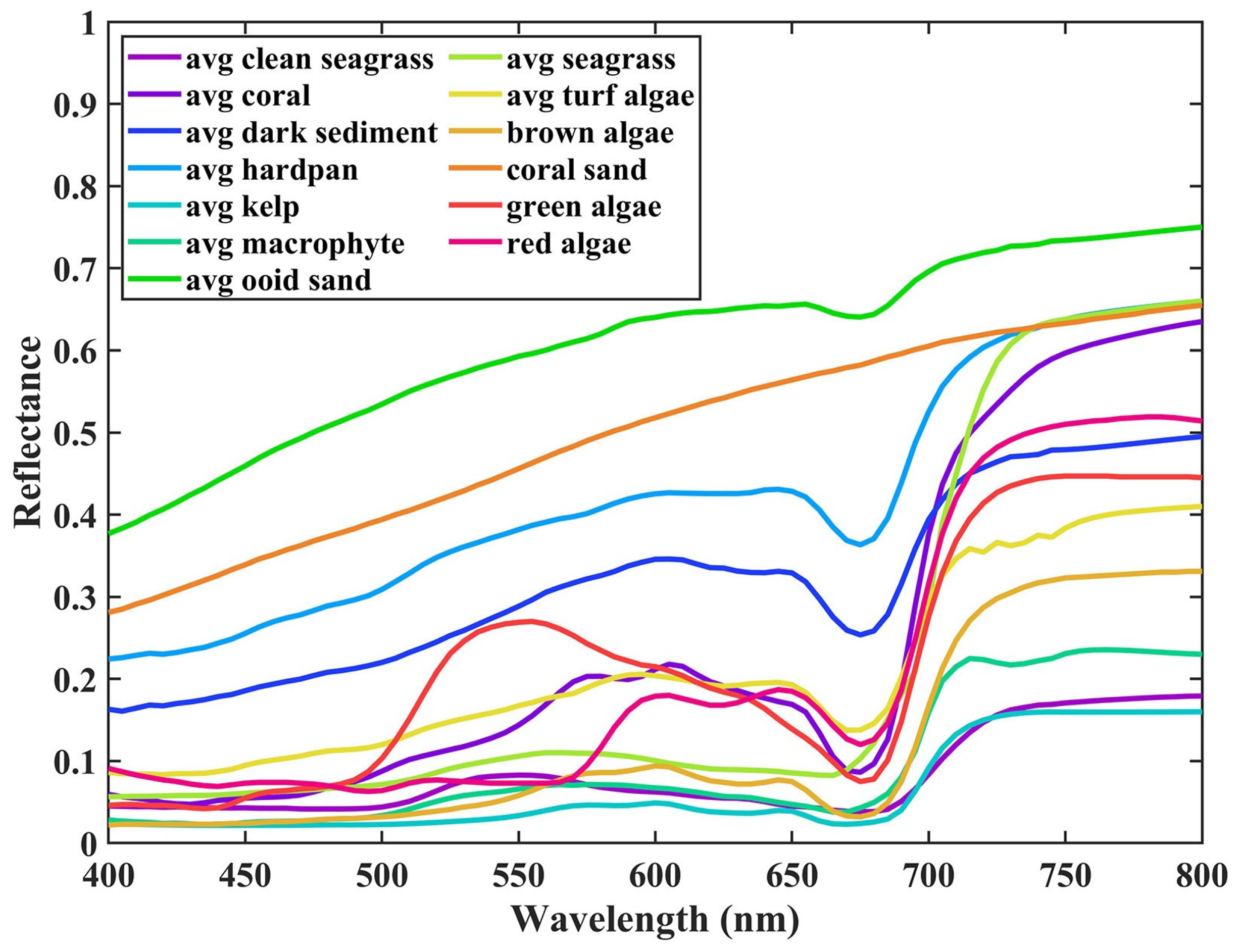
| Bottom reflectance | From user-supplied data (a totally of 145 types) |
| Range of water depth (m) | 0.01–10, random linear distribution |
| Acquisition Time | Accuracy | ||||
|---|---|---|---|---|---|
| Region | Sentinel-2 | ICESat-2 | N | MAPE | |
| Changpi Port | 21 February 2021 | 18 February 2021 | 273 | 0.1743 | 26.31% |
| Xincun Bay | 7 February 2020 | 30 January 2020 | 91 | 0.3172 | 38.06% |
| Huaguang Reef | 24 February 2020 | 20 February 2020 | 378 | 0.5386 | 14.12% |
Publisher’s Note: MDPI stays neutral with regard to jurisdictional claims in published maps and institutional affiliations. |
© 2022 by the authors. Licensee MDPI, Basel, Switzerland. This article is an open access article distributed under the terms and conditions of the Creative Commons Attribution (CC BY) license (https://creativecommons.org/licenses/by/4.0/).
Share and Cite
Wang, Y.; He, X.; Bai, Y.; Li, T.; Wang, D.; Zhu, Q.; Gong, F. Satellite-Derived Bottom Depth for Optically Shallow Waters Based on Hydrolight Simulations. Remote Sens. 2022, 14, 4590. https://doi.org/10.3390/rs14184590
Wang Y, He X, Bai Y, Li T, Wang D, Zhu Q, Gong F. Satellite-Derived Bottom Depth for Optically Shallow Waters Based on Hydrolight Simulations. Remote Sensing. 2022; 14(18):4590. https://doi.org/10.3390/rs14184590
Chicago/Turabian StyleWang, Yuxin, Xianqiang He, Yan Bai, Teng Li, Difeng Wang, Qiankun Zhu, and Fang Gong. 2022. "Satellite-Derived Bottom Depth for Optically Shallow Waters Based on Hydrolight Simulations" Remote Sensing 14, no. 18: 4590. https://doi.org/10.3390/rs14184590