Numerical Imaging of the Seabed and Acoustic Flares with Topography and Velocity Variance

Abstract

During seabed mapping, anomalous acoustic events in the seawater layer often degrade bathymetric quality. Acoustic-flare-like events that are induced by gas seepage occur accompanied by small seabed depressions known as pockmarks. In this study, we performed numerical imaging to verify whether acoustic flares are related to changes in the topography of the seabed. The input models assumed convex or concave upward structures which differ based on aperture size. The imaging study determined that acoustic flares appear because the sensing instrument measures the velocity changes in the water layer regardless of the seabed topography. Changes in the velocity of the seawater column can be caused by the concentration of suspended particles and the wave current above the seabed, but further quantification research is required.

1. Introduction

High–resolution bathymetric maps provide essential information for offshore transportation, fisheries, construction engineering, coast utilization, and understanding of depositional processes. Various remote sensing methods have been developed to build accurate bathymetric maps using smart technology. Conventional sensing, which is executed during water surveys, uses side-scan sonar and multi-beam instruments [1,2]. Even though data can be collected directly from the seabed during marine surveys, a large number of survey lines are required, and resources are dependent on sea conditions. To efficiently and productively sense a large area, airborne survey methods can be used to gather seafloor data at relatively shallow depths [3,4]. Additionally, satellite sensing can create regional bathymetric maps with a sufficient resolution over a large area [5,6]. Recent marine and airborne surveys used unmanned vehicles to obtain high-resolution images [7,8,9]. These remote sensing techniques can be affected by seafloor mapping conditions, such as rough seas, swell noise, water clarity, and other acquisition environments. To improve the data quality, a detailed understanding of the mapping conditions is required.

Based on remote sensing surveys on the seabed, massive gas seepages have been reported, showing flare-like events in the seawater [10,11,12]. Gas flares can affect bathymetric sensing or can be the target of sensing tasks in investigating gas migration. Unfortunately, the morphology of gas seepages differs due to fluid-generating mechanisms and tectonics or stratigraphy [12,13]. Several previous studies observed methane gas flares above the seafloor where gas hydrates are found in the subsurface. These gas flares are emitted through subsurface chimneys or fault structures [14,15,16]. The features of gas flares have been determined via direct sampling, monitoring, and simulations. Direct measurements address the type of emissions as well as time-variant characteristics of the flares [17,18]. Characterization methods such as defining the extent of gas flares, calculating the methane concentration, and observing seasonal variations have been conducted consistently for decades [19,20,21,22]. Recent modeling and simulations image gas flares with a fairly good resolution, which helps in preparing detailed bathymetric maps in the region of emissions and can identify the gas-charged zone [15,16,20,21]. Nevertheless, the micro-topographic changes that take place in the very shallow regions around gas vents are not well known and are difficult to detect with remote sensing. Commonly, gas emissions are found above the vents and are accompanied by small depressions in the seafloor morphology, i.e., pockmarks [11,13]. Pockmark distribution is not always consistent with gas flares, implying that they are correlated with deeper gas pathways [15]. If pockmarks affect gas flare images in the mapping sections, then a more detailed investigation is required both qualitatively and quantitatively.

Numerical reverse time migration (RTM) imaging can replicate seawater and subsurface structure images in a similar way to remote sensing surveys. An RTM technique based on wave propagation computation has been developed and used for imaging complex hydrocarbon reservoir prospects [23,24,25,26]. Using an assumed or known input acoustic/elastic velocity model of the subsurface medium, RTM can image various types of acoustic reflections that come from the subsurface [27]. Conventional RTM image depths are of several kilometers, making it a useful technique for imaging challenging deeper targets [28,29]. In this study, we focus on the acoustic imaging of shallow gas flares and seabed deformations within several tens of meters below the seafloor using the RTM technique. The method examines the variations in the topography and velocity of acoustic flare (AF) events which can be imaged via mapping sections. By verifying acoustic events via numerical imaging, remote sensing instruments and algorithms have an advantage in detecting/analyzing anomalies.

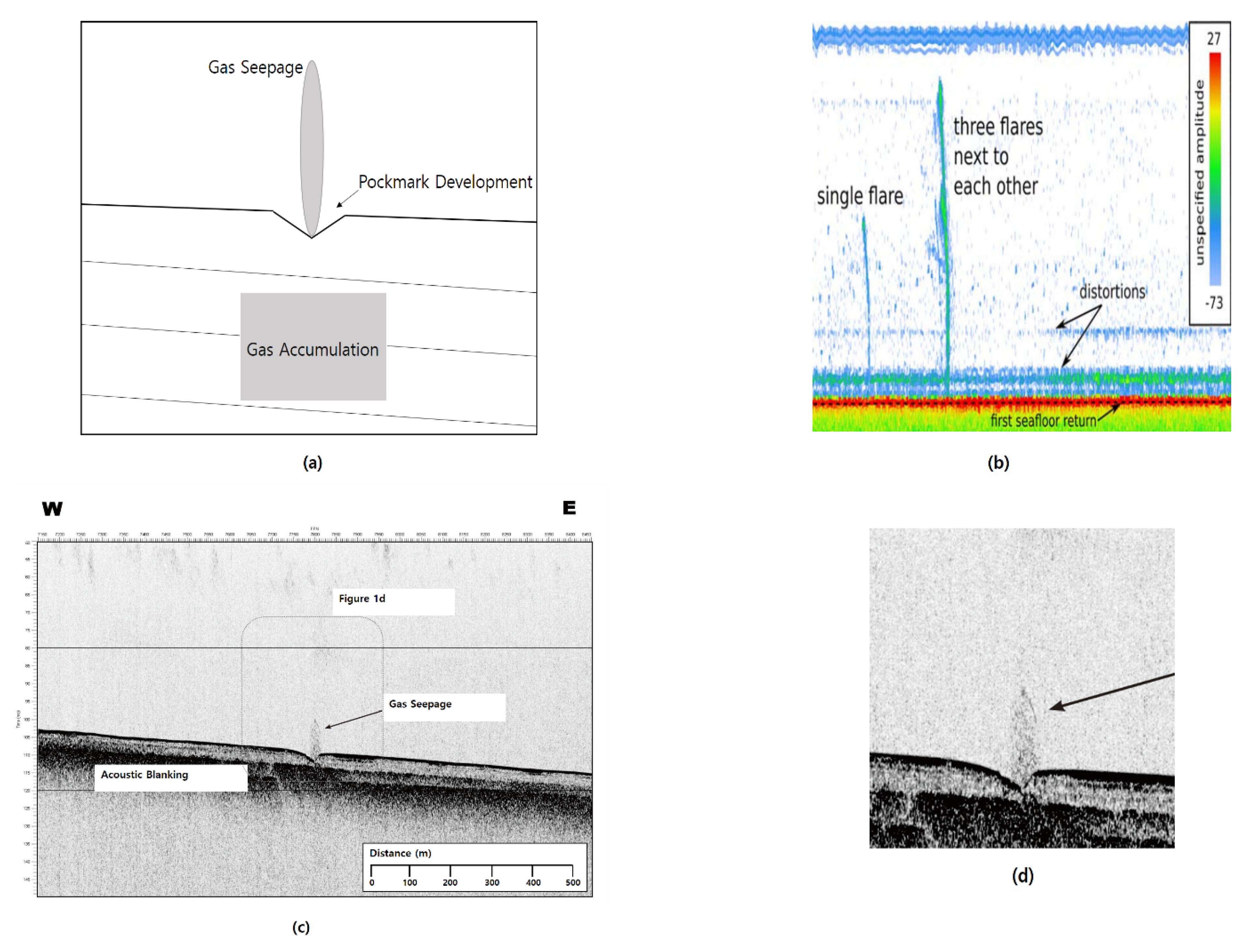
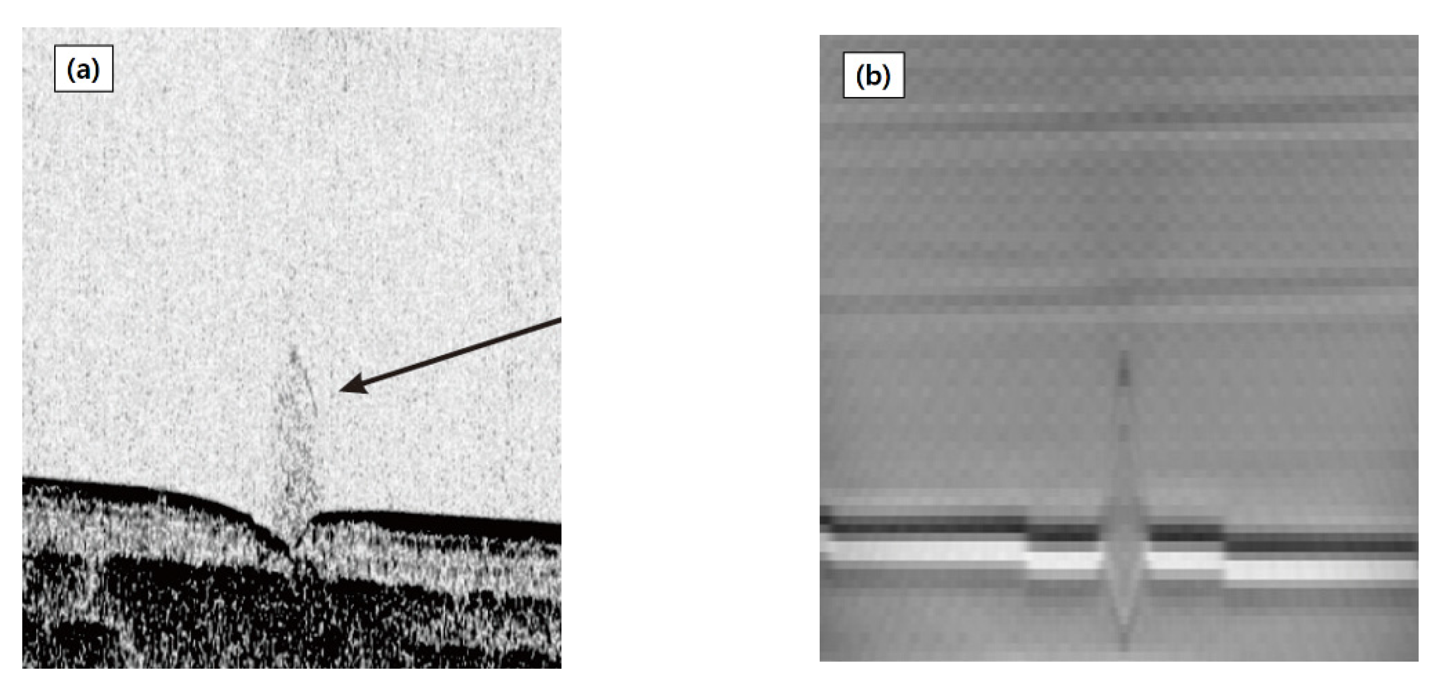
2. Aspects of Acoustic Flares

The gas flares observed in previous studies show various features which are difficult to define in terms of the position and scale of extent. Representative gas flares are found in different regions, such as in the Okhotsk Sea [10], the Gulf of California [11], offshore New Zealand [12], the Aegean Sea [13], and the Arctic Ocean [15]. Gas flares rise from the seabed and travel up to several hundred meters in the seawater [10,30] or even up to thousands of meters high in the region of mud volcanos [31]. The majority of gas flares are associated with features such as pockmarks, faults/fractures, blank zones, chimneys, and vents in the subsurface [11,13]. The most well-known flare mechanism is the dissolved methane hydrate that seeps into the seawater [32,33]; however, any kind of thermodynamic or biogenic gas can escape into the seawater.

To resolve gas seepage, interpretation via different remote sensing techniques is needed. Because the appearance of flares varies depending on the remote sensing instruments, a comprehensive analysis is crucial. Sensing using a single-beam echo-sounder can image gas flares in vertical sections. Direct emissions can be captured using side-scan sonar instruments and areal distribution can be well observed with a multibeam echo-sounder (MBES) in high-resolution images. A sub-bottom profiler (SBP) survey displays seafloor images with a subsurface structure. The high–resolution seismic airgun data, which provide good images of the subsurface, cannot display the gas flares in seawater regions clearly [16,33].

The reason flares are not clear in conventional seismic sections is probably because of the differences in the frequency components. It has been reported that AFs look like vertical pillars and develop as gas seeps from vents on the seabed above gas accumulation [13]. Figure 1a shows a typical gas seepage shape with a pockmark in the mapping section. Because specific surveys use equipment of different frequencies, the sizes and shapes of the flares and/or pockmarks could vary. The flare shows a sharp contrast to the seawater layer in remote sensing sections determined via an echo-sounder survey [30]. In MBES-determined sections, AFs are clearer and often distributed in clusters (Figure 1b). An SBP section can display AFs and associated subsurface structures because the survey can record signals from deeper sediment reflections (Figure 1c). In magnified SBP sections, the gas seepage is clearly observed as an acoustic flare above the pockmark development (Figure 1d).

Among these characteristics, there is insufficient information to clearly understand the relationship between the shape of the seafloor vent and a flare. Although seafloor vents or pockmark features are often associated with flares, their shapes are poorly understood. A detailed seabed topology may affect the shape and clustering of AFs. Based on the observations of AFs in previous studies [13], we are motivated to construct numerical model inputs.

3. Numerical Modeling Results

This section describes the principle of RTM and the test results of topographic and acoustic variant input models for RTM imaging of seawater and subsurface. The topographic variant model corresponds to the size of the aperture and upward/downward morphological changes. The velocity variant model is constructed by putting artificial anomalies in seawater regions and assuming that the AF has a column shape.

3.1. Reverse Time Migration (RTM)

Numerical modeling can simulate survey sections derived from remote sensing by means of theoretical applications of computational wave propagation. Based on recent developments in computer science, the finite difference method (FDM) and finite element method (FEM) are able to solve wave equations in the time and frequency domain [34,35].

The acoustic wave equation can be written as Equation (1):

$$\frac{1}{v^2}\frac{{\partial }^{2}P\left(x,y,z,t\right)}{\partial t^2}=\frac{{\partial }^{2}P\left(x,y,z,t\right)}{\partial x^2}+\frac{{\partial }^{2}P\left(x,y,z,t\right)}{\partial y^2}+\frac{{\partial }^{2}P\left(x,y,z,t\right)}{\partial z^2}+f$$

(1)

where $\mathrm{P}\left(\mathrm{x},\mathrm{y},\mathrm{z}\right)$ is the wavefield, $\mathrm{v}$ is the acoustic velocity, $\mathrm{t}$ is the time variable, x, y, z are the spatial variables, and $\mathrm{f}$ is the source wavelet.

Using forward wave propagating methods, RTM is introduced to generate subsurface images with a high resolution [36]. RTM cross-correlates two wavefields: source-propagated (Figure 2a) and receiver-back-propagated (Figure 2b). The summation image represents the best-correlated image from perturbation by reflective structure (Figure 2c). The image from RTM can be expressed by Equation (2):

$$\mathrm{I}\left(\mathrm{x},\mathrm{y},\mathrm{z}\right)={\displaystyle \sum }{\displaystyle \sum }S\left(x,y,z,t\right)R\left(x,y,z,t\right)$$

(2)

where $\mathrm{I}\left(\mathrm{x},\mathrm{y},\mathrm{z}\right)$ is the image of the given grid position, $\mathrm{S}\left(\mathrm{x},\mathrm{y},\mathrm{z},\mathrm{t}\right)$ is the source wavefield propagation, and $\mathrm{R}\left(\mathrm{x},\mathrm{y},\mathrm{z},\mathrm{t}\right)$ is the receiver wavefield propagation.

Mapping subsurface reflectivity is determined via wave propagation through an input velocity model with a designed ray path from source to receiver array [27]. Because RTM calculates all the reflected wavelets, it requires accurate subsurface velocity information [25].

Because RTM generates the best solutions for seismic responses, including acoustic flares and subtle morphology changes, this study used time domain pre-stack RTM for simulating the subsurface. For RTM, we set a uniform square grid in which each square was spaced 1 m apart and used a sampling interval of 0.2 ms, resulting in a 0.6 s total recording time that generated 3000 time samples. The dimensions of the numerical model consist of a distance axis and a depth axis that is 401 by 201 grid points and simulates the whole seawater and subsurface for a 400 × 200 m rectangular domain. The parameters for the numerical model were selected according to those required for an SBP survey, which can have a maximum frequency of 370 Hz which is larger than the 200 Hz of a normal air-gun survey [37,38]. The limit to numerical modeling performance is the quality of the processing which depends on the accuracy of the input data. In our method, the time interval is reduced from 0.28 to 0.20 ms in order to reduce the dispersion error. To meet a stability condition, we used a grid number of 20 [39].

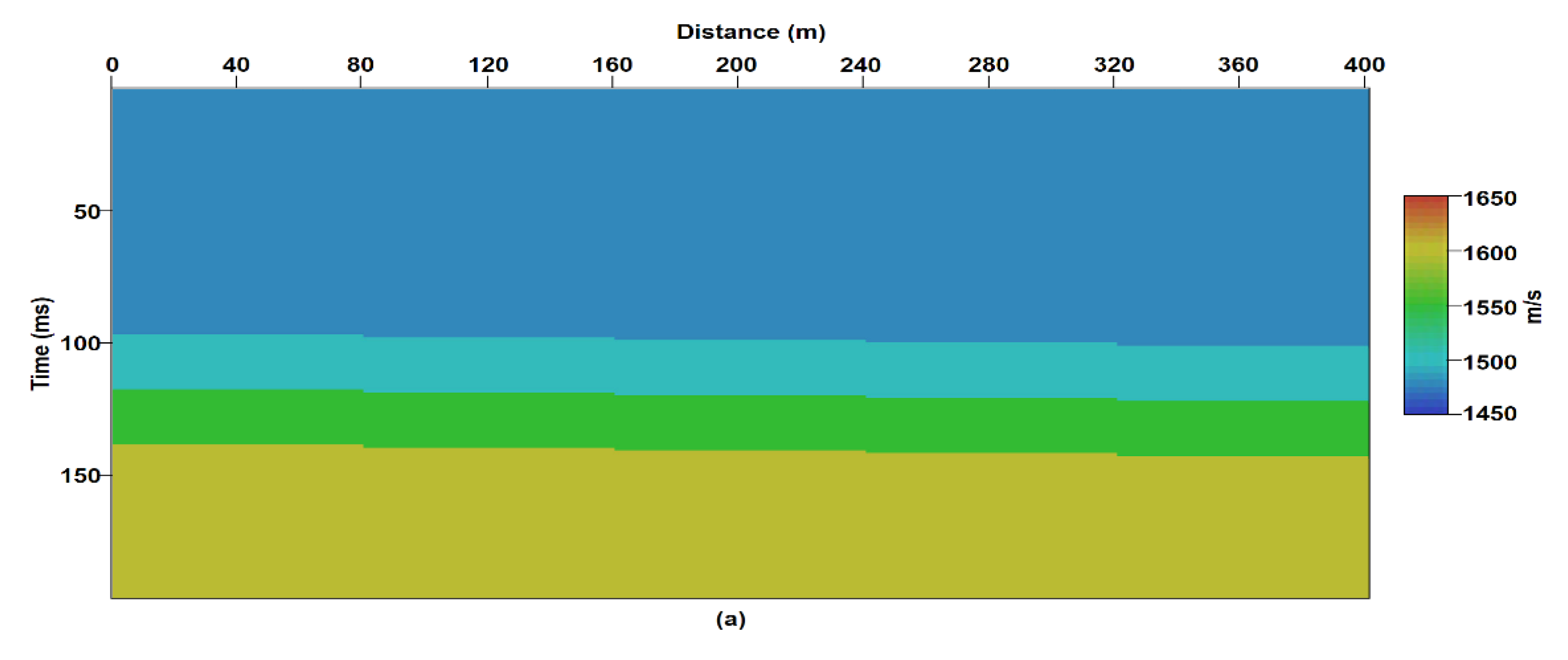
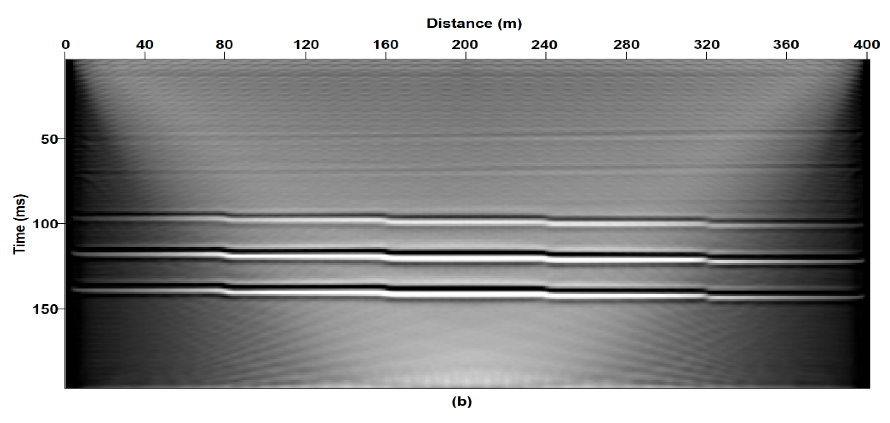
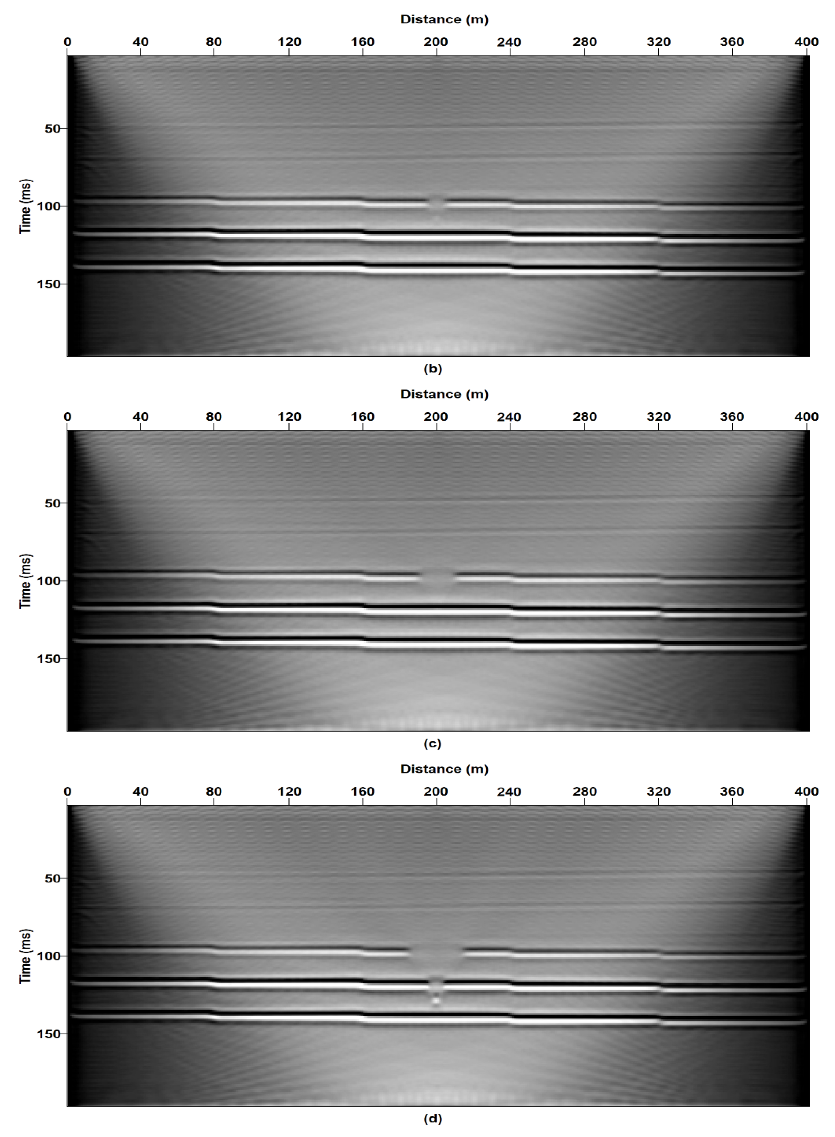
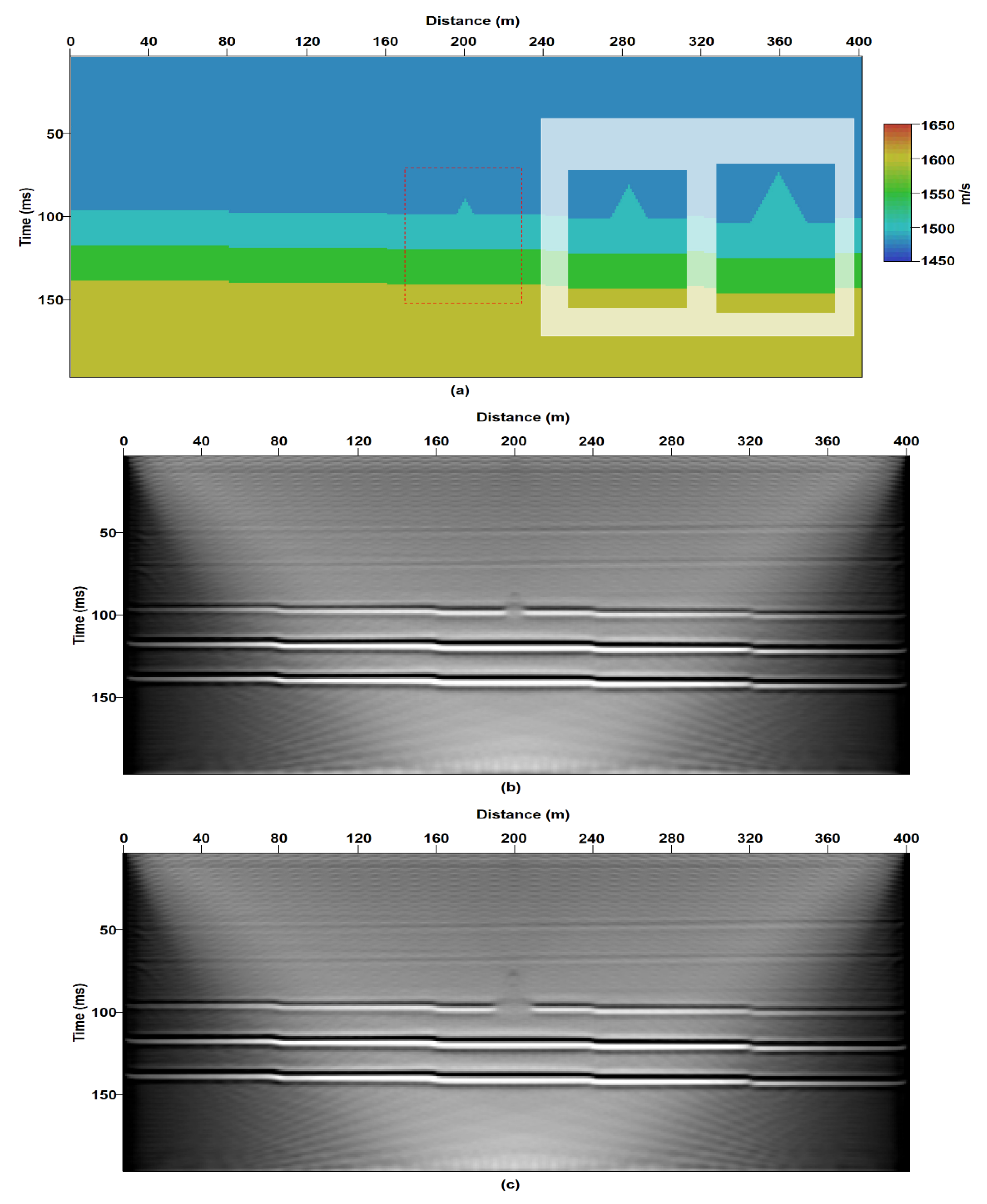
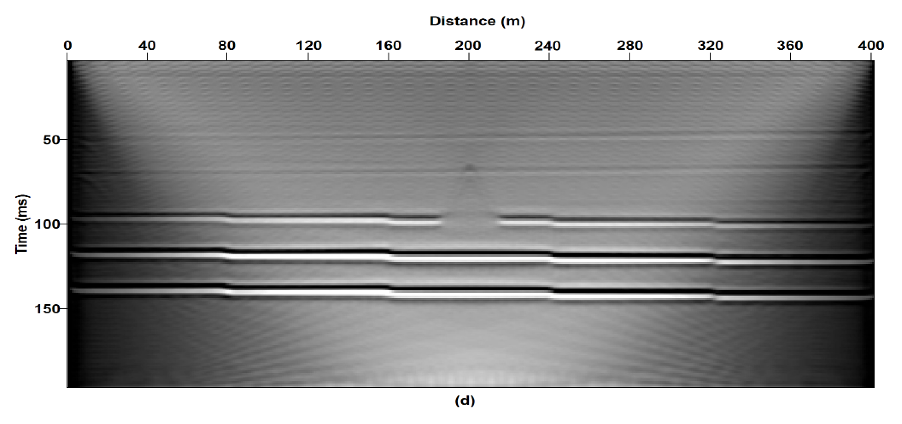
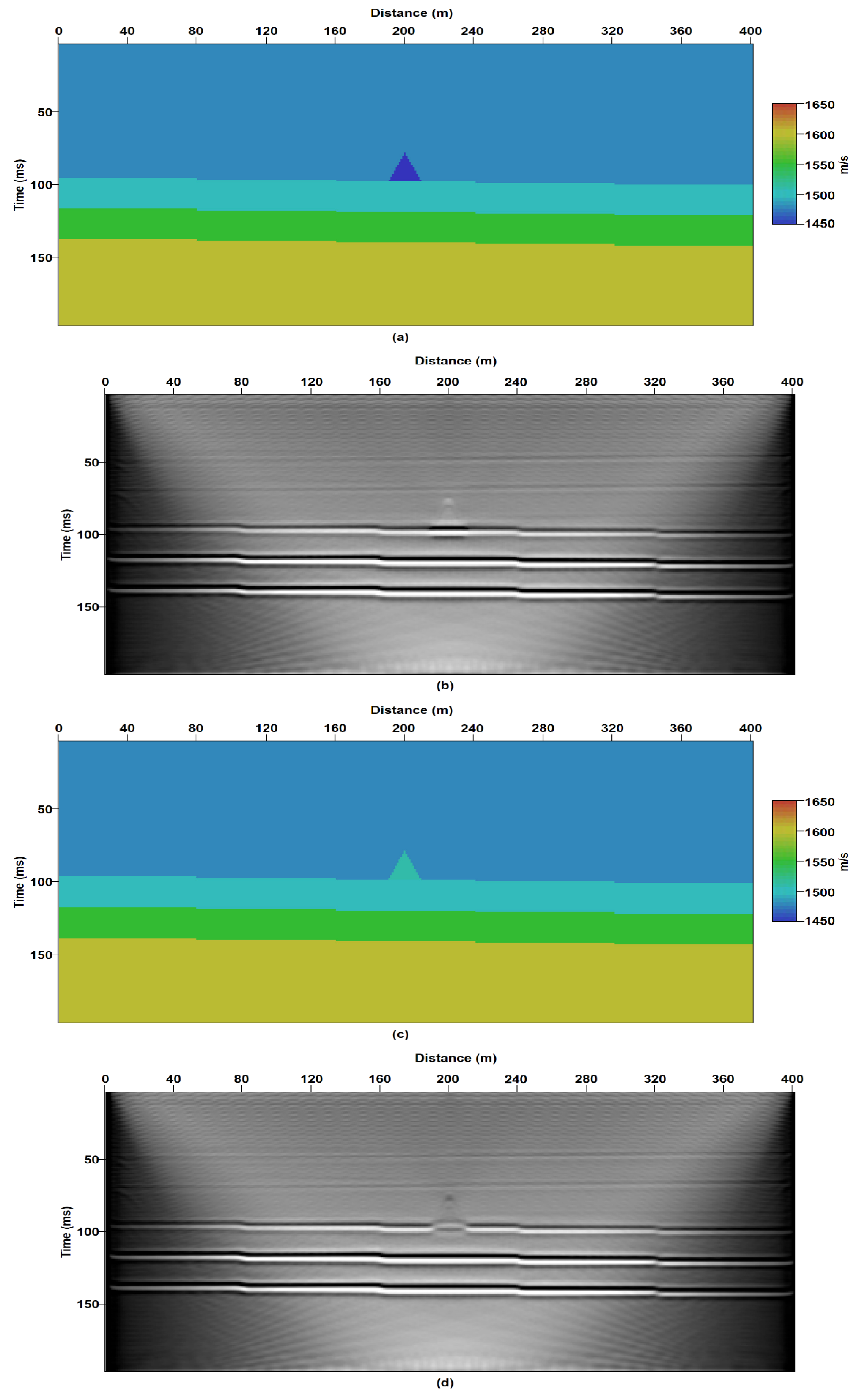
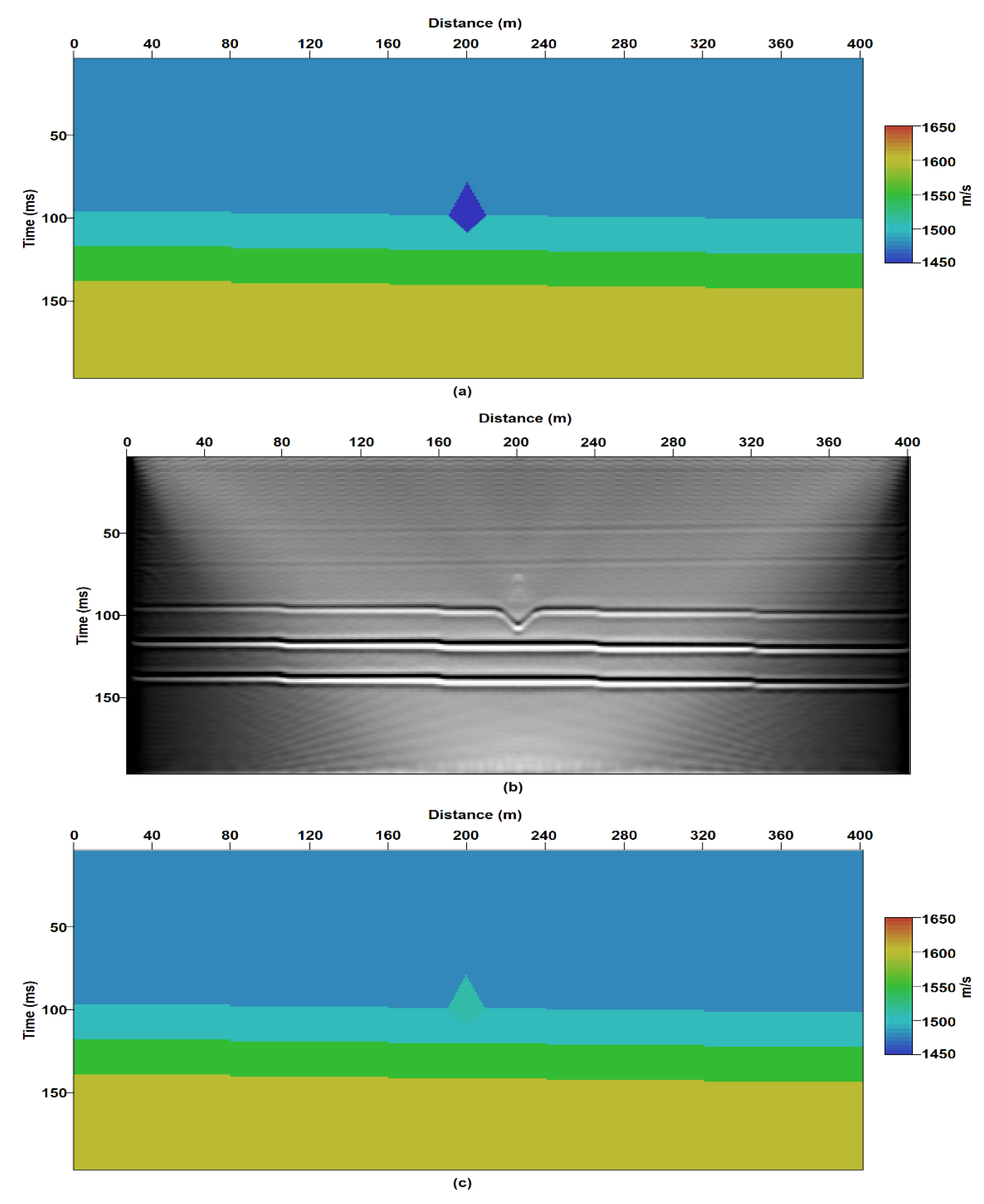
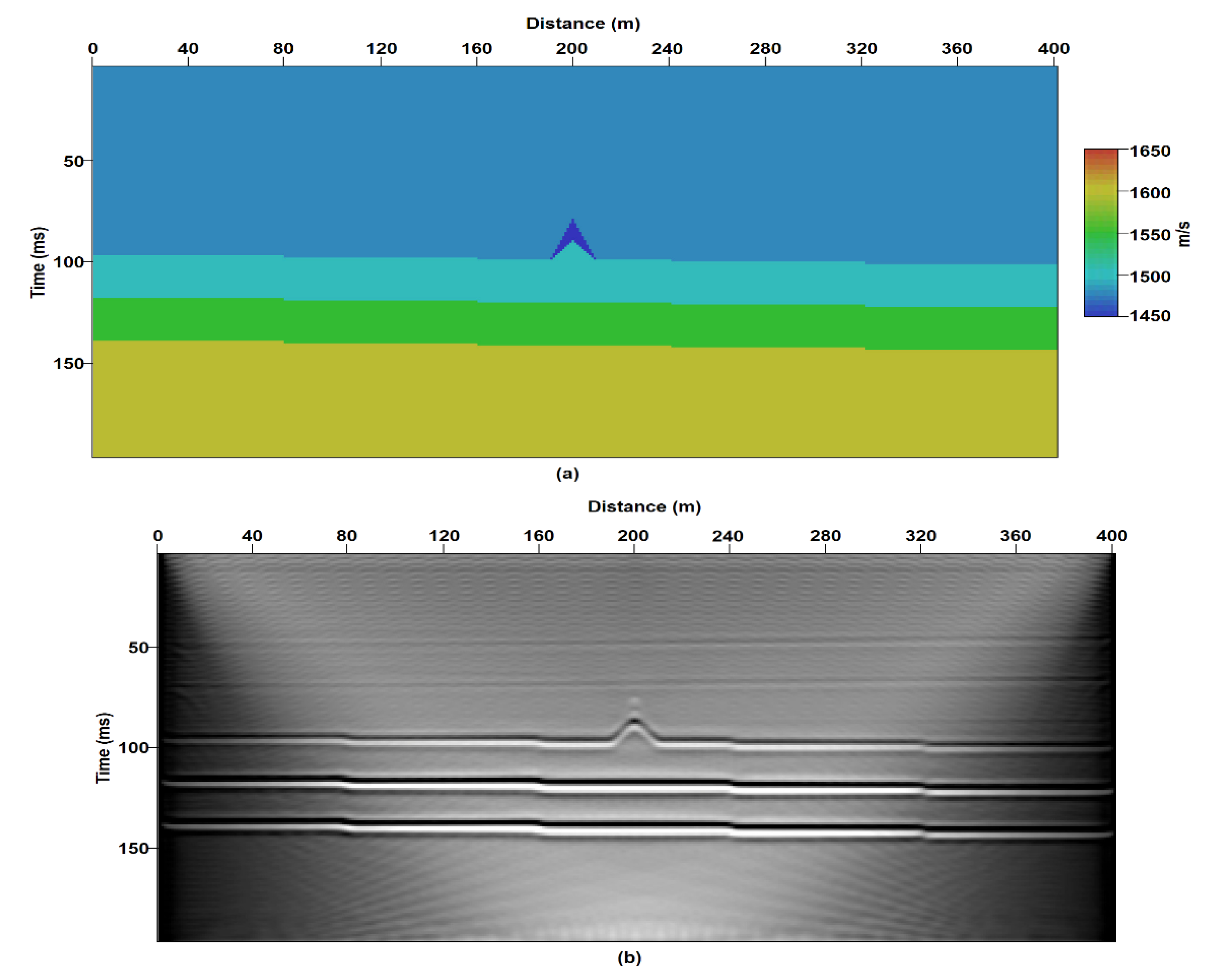
3.2. Topographic Variant Model

The signals that are acquired through remote sensing reflect geophysical properties; here, the studied properties are the acoustic velocity of seawater and subsurface sediment, so we manipulated the input velocity to derive the numerical image-simulated survey sections. We used input velocity models to check the validity and to change the morphological effects that depend on the seabed having a flat, concave, and convex shape. There are three types of input models, including a flat, pockmark, or mound shape. The latter two have a scale to determine the variations in morphological changes, classifying them as 10, 20, and 30 m anomalies (

Table 1. Tested input models for morphological variations.

Model Name	Variables	Objective
Flat	Acoustic velocities of seawater and three sediment layers	Validation
Pockmark	Size (10/20/30 m)	Depression effect
Mound	Size (10/20/30 m)	Protrusion effect

).

The first input velocity model is a flat-layered model of the shallow sediment in the unconsolidated layer to validate the RTM application. The assumed P-wave velocities of the layers are 1480 m/s for the seawater layer and 1500, 1550, and 1600 m/s for the layers spanning from the top to the bottom (Figure 3a). All of the layers are inclined from left to right and deepen by 5 m over the whole distance of 400 m (0.7 degrees inclination). The RTM used 40 virtual sources to propagate the seismic wavelet at the surface and was evenly spaced over 401 grid points (sources are placed at every 10 grid points).

The RTM results obtained with the flat model show that the interfaces of the layers are imaged with their inclinations at the correct depth (Figure 3b). In the seismic migration section, the seawater layer and second and third layers are shown in solid black and white lines that represent positive and negative amplitude reflection signals.

The pockmark model was designed to test the morphological effects in remote sensing surveys where depressions are located on the seabed in the unconsolidated muddy sediment. In the model, the acoustic velocities from the seabed to the deepest layer are the same as those in the flat model, but there is a small depression at the center of the seabed (Figure 4a). The size of the pockmark can vary, and this is represented by a triangular shape that is 10, 20, or 30 m in size (width and height equally) for small, medium, and large depressions, respectively. We chose the shape of the pockmark as triangular because the pockmark should have an aperture that decreases with depth and tapers at the boundary. The shape of the pockmark can be triangular, round, or any other polygon-type shape that has an aperture which decreases with depth in the numerical velocity input. The effect of a depression shape in remote sensing surveys is the artifact of diffraction [40]. Regarding the grid number of numerical examples, we reasoned that a triangular shape is the best- shape to represent a diffraction event rather than a rectangular or round shape. Moreover, a triangular shape is similar to the schematic diagram of the pockmark presented in Figure 1a.

In the RTM results, no apparent heterogeneous events were observed in the first and second layers (Figure 4b–d). The interfaces between the layers appear correct on the migrated sections where they would be in the input velocity models, but the shape of the pockmark is not clearly seen at the depth of the seabed. The image at the contact layer between the seawater and the seabed can be blurred as a result of a loss in the reflection signal during RTM wave propagation. The RTM results demonstrate the existence and the size of depressions at the seabed and demonstrate that pockmarks cannot create acoustic events in sea-water.

Since there were no obvious abnormalities in the RTM images of the seawater region near the pockmark, we conducted tests using a mound model, which is used when there is a protrusion on the seabed. The mound model has the same velocity layers and adds morphological change with protrusions that are represented by triangular shapes that are 10, 20, and 30 m in size for small, medium, and large protrusions (Figure 5a). The RTM images show all of the interfaces between the subsurface layers that describe the true velocity models (Figure 5b–d).

The results of both the pockmark and mound models demonstrate that the interfaces between the seawater and the seabed are reduced at the distance at which morphological anomalies are visible. This implies the possibility of the vertical artifact being observable in the remote sensing section where there is discontinuity on the horizontal axis. The traveling direction of the numerical source is vertical so that a horizontal object or anomaly is clearer than a vertical structure in the RTM images. It can be determined that anomalies in physical velocity are the main factors influencing events in the mapping section, i.e., acoustic flare events. This result means that the events that appear above the seabed in this section are not due to changes in the adjacent terrain. In other words, the velocity changes in the area that coincides with the location where the event appears is expressed as an artifact in the remote sensing section.

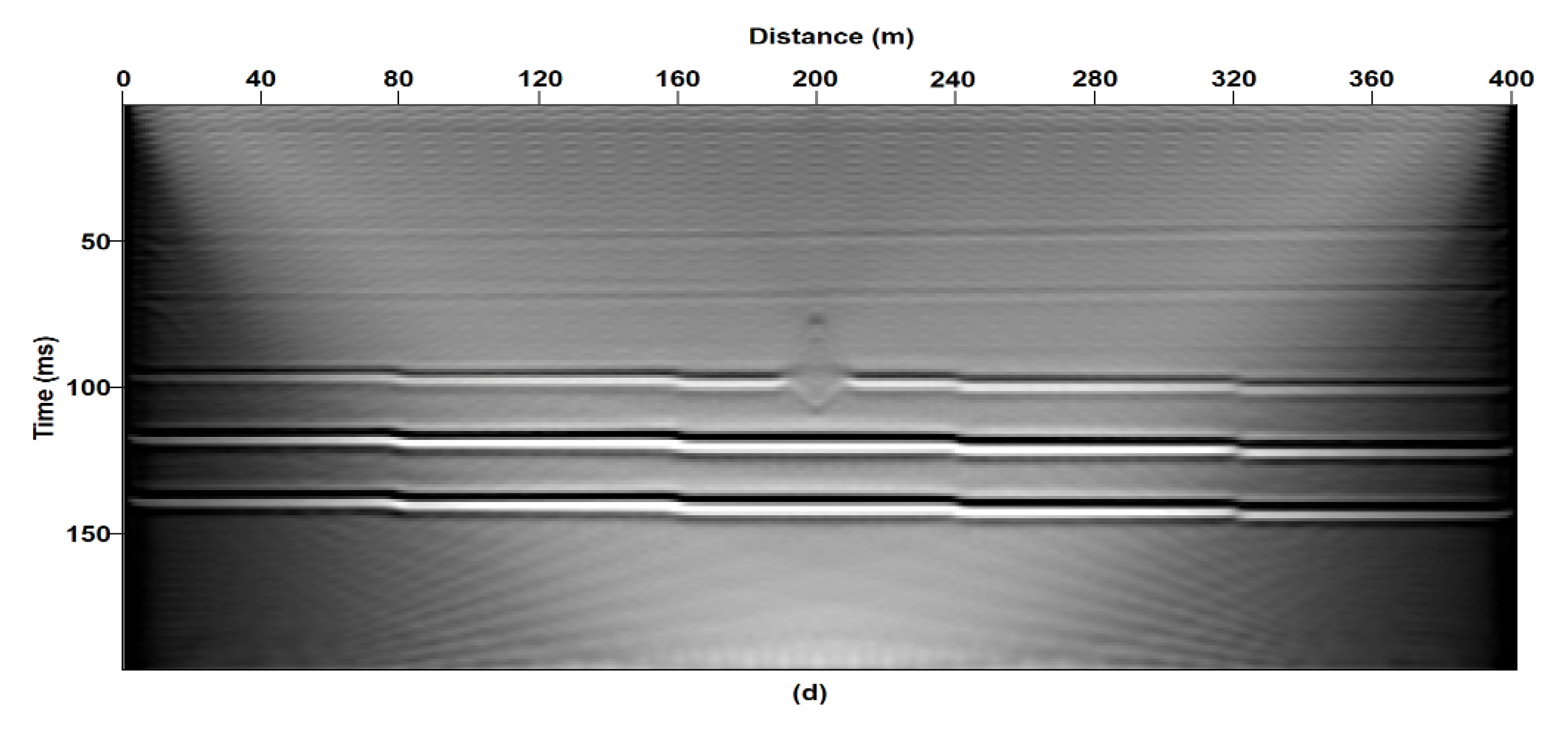
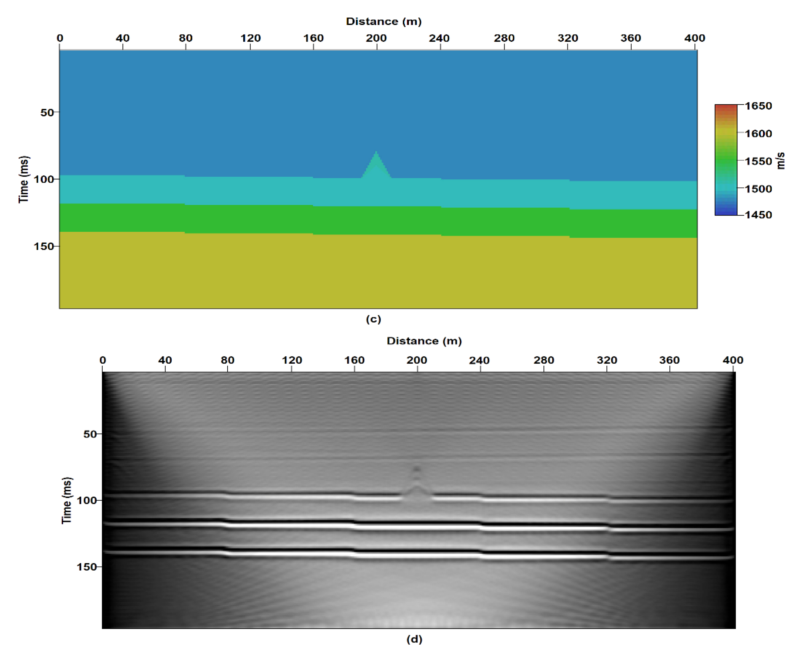
3.3. Acoustic Variant Model

Because migration images are dependent on changes in the input velocity, we added artificial velocity perturbations in the water column region. The region of perturbation is represented by triangular grid points that are 10 m wide and 20 m high and assumes that a gas flare is 10 m thick and rises 20 m above the seabed. Since gas elution diffuses and disappears from the bottom to the top, the shape of the column was assumed to be a triangle which is wider at the bottom and narrower at the top. We assumed that velocity perturbations could be caused by gas bubbles and particle oscillation effects, which would change the velocity by +30 and −30 m/s in the triangular region (

Table 2. Tested input models for acoustic velocity variations.

Model Name	Velocity Change	Objective
Velocity variant at flat	Negative (−30 m/s) and positive (+30 m/s)	Perturbation of seawater above seabed
Velocity variant at pockmark	Negative (−30 m/s) and positive (+30 m/s)	Perturbation with pockmark
Velocity variant at mound	Negative (−30 m/s) and positive (+30 m/s)	Perturbation with mound

). The local decrease and increase in seawater velocity assumes a large number of dissolved air bubbles, and a state in which solid particles are suspended in the water column region.

In general, numerical methods assume that the seabed has mild topography and a constant velocity of 1500 m/s. Since velocity changes in seawater are relatively small compared to wave propagation velocity changes in the sediment strata, it is common not to assume that there are velocity changes in the seawater when using conventional RTM. Our model aims to image acoustic events in a similar seawater column zone; thus, we added positive and negative variations of 30 m/s, which represent minor changes in the seawater speed. These slight variations in sound velocity are the result of pressure changes or turbidity being affected by the emission of gas bubbles and solid particles. It has been reported that the sound velocity in a liquid with gas bubbles will be less than in a liquid without bubbles [41]. Additionally, previous experiments have reported an increase in wave transmissibility via gas bubbles and solid particles [42,43].

When variations in the acoustic velocity variant were added to the flat model, the RTM results showed a vertically anomalous image that looks like acoustic flares (Figure 6). Both negative (Figure 6a) and positive (Figure 6c) velocity changes affected the RTM images (Figure 6b,d) when the velocity changes took place above the seabed. A polarity change was observed in the seabed when reflectivity decreased from 1510 m/s in perturbed seawater to 1500 m/s at the first sedimentary layer in the area where acoustic variation was observed (Figure 6d).

In the pockmark model, consistently negative and positive velocity perturbations caused by gas bubbles or solid particles show gas-flare-like events in the area where there is acoustic variation in the seabed as well as pockmark morphology (Figure 7). Therefore, the acoustic events in mapping sections obtained from remote sensing surveys are phenomena that occur because the speed of the seawater is measured abnormally in a specific region independently of the pockmark or changes in the seabed topography. In addition, depending on whether the speed of the seawater layer measured by the remote sensor is increasing or decreasing, the polarity of the seafloor signal may be changed or blurred, so it may not be visible. The dimming effect in the subsurface layer is consistent with reflectivity changes observed in the gas-charged zone [44,45].

The results of the velocity variant with mound models show a larger superimposed disturbance in the water column region than the pockmark model (Figure 8). This disturbance is due to the presence of a velocity at the mound position that is greater than the seismic velocity of the seawater at the water column position. If the mound topography does not exist and the velocity of the seawater changes significantly compared to the surrounding area, a similar pattern is expected. The results of the hydrodynamic numerical experiment proved that the wave causes negative and positive velocity changes in a column composed of air and gas [46]. This means that if no significant differences are observed between the seawater velocity near the seabed and the velocity of the sedimentary layers on the seabed, then they can be seen together in the remote sensing section. In fact, we were able to observe this pattern continuously in the echo-sounder section.

Comparing the SBP section with the numerical modeling results shows that the gas flare (Figure 9a) is similar to the acoustic variation caused by velocity perturbations (Figure 9b). The shape of the acoustic flare is obvious above the seabed and is represented by a small depression.

4. Discussion

We found an event related to acoustic perturbations via numerical imaging that may be able to be observed in mapping sections derived using remote sensing techniques. RTM can not only image the subsurface structure but can also image velocity perturbations that are assumed to be present in anomalous areas, i.e., in seawater regions when a specific input velocity model is designed. The reason that our results were able to reproduce acoustic events is that the input velocity includes subtle velocity changes for the optimized region rather than the general input model applied to the conventional RTM.

If there is a gas bubble emitted above the seabed, the measurements of the seawater velocity may vary subtly, affecting bathymetric maps. The RTM results imply that the gas flare seen in the MBES and SBP sections can also be confirmed using seismic airgun data with high-frequency components. This means that remote sensing parameters should be optimized according to the characteristics of the target to be measured. The observation of acoustic flares will be easier if the maximum frequency of the high-resolution survey can record up to 200 Hz or more. Furthermore, it is preferable to refer to the value in setting the input parameter of the frequency bandpass filter applied in the data processing process.

Furthermore, the shape of a gas flare can be arbitrary in the water column, and this can be addressed by using a finer grid during water layer simulations when the temperature and pressure information is provided [47,48]. A high temperature and pressure are measurable at points of highly concentrated gas emissions, which indicates a huge amount of dissolved gas with a flare event. The temperature and pressure information does not directly affect the RTM result, and the measured seawater velocity change due to the ejected gas indirectly affects the RTM image. Thus, a given velocity that is measured by sampling temperature and pressure at a specific location will affect the accuracy of the RTM image. The latest numerical methods use more input information to improve the resolution of three-dimensional target images [49,50]. With detailed gas flare information, RTM can derive more accurate AF boundaries. Additionally, quantitative velocity change can be monitored using numerical methods. It is possible to quantitatively interpret the gas emissions using time-lapse seismic monitoring techniques that are used for enhanced oil recovery or the geological storage of carbon dioxide [51,52].

Minute velocity changes in the seawater layer must be continuously taken into account when using remote sensing technology to construct accurate bathymetric maps. Autonomous underwater vehicles (AUVs)/unmanned aerial vehicles (UAVs) are only able to provide high-quality seafloor maps when they detect anomalies in the seawater velocity during the process of recognizing acoustic-flare-like events. In addition, the accumulated knowledge of the characteristics of the remote sensing medium can contribute to improving the accuracy of seabed exploration by providing good input data for the machine learning process.

5. Conclusions

Acoustic events that can be observed on remote sensing maps in seawater were numerically imaged using RTM with respect to the input model. The input model assumed the acoustic velocity of both the seawater and the subsurface layer where acoustic waves are propagated and reflected. The flat model verified that RTM can image simple geologic structures with a sufficient resolution using the field scale in remote sensing technologies.

The topographic variation model consisted of convex (pockmark) and concave (mound) anomalies on the seabed that were 10, 20, and 30 m in size. The RTM results showed that the shape observed in the morphological images does not affect acoustic flares. This model proves that the seabed can be mapped with its original features by means of remote sensing if there are no perturbations caused by gas seepage.

The acoustic variation model considered a perturbation of 30 m/s in the background velocity of 1480 m/s at normal acoustic water speed, assuming a smaller velocity change than the conventional RTM. The resultant images described artificial events in the water column area that looked similar to the gas flares observed in the remote sensing section. These results imply that acoustic flares can be observed via remote sensing when specific velocity changes are observed in the seawater layer. The changes in seawater velocity are likely induced by the movement of suspended particles and the current of the seawater.

References

1. Pryor, D.E. Theory and test of bathymetric side scan sonar. In Proceedings of the Oceans’88 ‘A Partnership of Marine Interests’, Baltimore, MD, USA, 31 October–2 November 1988. [Google Scholar]
2. Biju-Duval, B.; Le Quellec, P.; Mascle, A.; Renard, V.; Valery, P. Multibeam bathymetric survey and high resolution seismic investigation on the Barbados ridge complex (Eastern Caribbean): A key to the knowledge and interpretation of an accretionary wedge. Tectonophysics 1982, 86, 275–304. [Google Scholar] [CrossRef]
3. Guenther, G.C.; Cunningham, A.G.; LaRocque, P.E.; Reid, D.J. Meeting the Accuracy Challenge in Airborne Lidar Bathymetry. In Proceedings of the 20th EARSeL Symposium: Workshop on Lidar Remote Sensing of Land and Sea, Dresden, Germany, 16–17 June 2000; National Oceanic Atmospheric Administration: Washington, DC, USA, 2000. [Google Scholar]
4. Roberts, A.C.B. Shallow water bathymetry using integrated airborne multi-spectral remote sensing. Int. J. Remote Sens. 1999, 20, 497–510. [Google Scholar] [CrossRef]
5. Smith, W.H.; Sandwell, D.T. Bathymetry prediction from dense satellite altimetry and sparse shipboard bathymetry. J. Geophys. Res. 1994, 9, 21803–21824. [Google Scholar] [CrossRef]
6. Casal, G.; Hedley, J.D.; Monteys, X.; Harris, P.; Cahalane, C.; McCarthy, T. Satellite-derived bathymetry in optically complex waters using a model inversion approach and Sentinel-2 data. Estuar. Coast. Shelf Sci. 2020, 241, 106814. [Google Scholar] [CrossRef]
7. Agrafiotis, P.; Skarlatos, D.; Georgopoulos, A.; Karantzalos, K. Shallow water bathymetry mapping from UAV imagery based on machine learning. Int. Arch. Photogramm. Remote Sens. Spat. Inf. Sci. 2019, XLII-2/W10, 9–16. [Google Scholar] [CrossRef]
8. Mandlberger, G.; Hauer, C.; Wieser, M.; Pfeifer, N. Topo-Bathymetric LiDAR for monitoring river morphodynamics and Instreamhabitats-A case study at the Pielach river. Remote Sens. 2015, 7, 6160–6195. [Google Scholar] [CrossRef]
9. Mandlberger, G. A review of airborne laser bathymetry for mapping of inland and coastal waters. Hydraul. Nach. 2020, 116, 6–15. [Google Scholar]
10. Salomatin, A.S.; Yusupov, V.I. Seabed and seawater column investigations by acoustic remote sensing. In Proceedings of the XIX Session of the Russian Acoustical Society, Nizhny Novgorod, Russia, 24–28 September 2007. [Google Scholar]
11. Canet, C.; Prol-Ledesma, R.M.; Dando, P.R.; Vazquez-Figueroa, V.; Shumilin, E.; Birosta, E.; Sanchez, A.; Robinson, C.J.; Camprubi, A.; Tauler, E. Discovery of massive seafloor gas seepage along the Wagner Fault, northern Gulf of Califonia. Sediment. Geol. 2010, 228, 292–303. [Google Scholar] [CrossRef]
12. Klauke, I.; Weinrebe, W.; Petersen, C.J.; Bowden, D. Temporal variability of gas seeps offshore New Zealand: Multi-frequency geoacoustic imaging of the Wairarapa area, Hikurangi margin. Mar. Geol. 2010, 272, 49–58. [Google Scholar] [CrossRef]
13. Dondurur, D.; Cifci, G.; Drahor, M.G.; Coskun, S. Acoustic evidence of shallow gas accumulations and active pockmarks in the Izmir Gulf, Aegean sea. Mar. Petrol. Geol. 2011, 28, 1505–1516. [Google Scholar] [CrossRef]
14. Jin, Y.K.; Kim, Y.; Baranov, B.; Shoji, H.; Obzhirov, A. Distribution and expression of gas seeps in a gas hydrate province of the northeastern Sakhalin continental slope, Sea of Okhotsk. Mar. Petrol. Geol. 2011, 28, 1844–1855. [Google Scholar] [CrossRef]
15. Rajan, A.; Mienert, J.; Bunz, S. Acoustic evidence for a gas migration and release system in Arctic glaciated continental margins offshore NW-Svalbard. Mar. Petrol. Geol. 2012, 32, 36–49. [Google Scholar] [CrossRef]
16. Dewangan, P.; Sriram, G.; Kumar, A.; Mazumdar, A.; Peketi, A.; Mahale, V.; Reddy, S.S.C.; Babu, A. Widespread occurrence of methane seeps in deep-water regions of Krishna-Godavari basin, Bay of Bengal. Mar. Petrol. Geol. 2021, 124, 104783. [Google Scholar] [CrossRef]
17. Von Deimling, J.S.; Greinert, J.; Chapman, N.R.; Rabbel, W.; Linke, P. Acoustic imaging of natural gas seepage in the North Sea: Sensing bubbles controlled by variable currents. Limnol. Oceanogr. Methods 2010, 8, 155–171. [Google Scholar] [CrossRef]
18. Greinert, J. Monitoring temporal variability of bubble release at seeps: The hydroacoustic swath system GasQuant. J. Geoph. Res. 2008, 113, C07048. [Google Scholar] [CrossRef]
19. Kannberg, P.K.; Trehu, A.M.; Pierce, S.D.; Paull, C.K.; Caress, D.W. Temporal variation of methane flares in the ocean above Hydrate Ridge, Oregon. Earth Plan. Sci. Lett. 2013, 368, 33–42. [Google Scholar] [CrossRef]
20. Gentz, T.; Damm, E.; Von Deimling, J.S.; Mau, S.; McGInnis, D.F.; Schluter, M. A water column study of methane around gas flares located at the West Spitsbergen continental margin. Cont. Shelf. Res. 2014, 72, 107–118. [Google Scholar] [CrossRef]
21. Urban, P.; Koser, K.; Greinert, J. Processing of multibeam water column image data for automated bubble/seep detection and repeated mapping. Limnol. Oceanogr. Methods 2017, 15, 1–21. [Google Scholar] [CrossRef]
22. Longo, M.; Lazzaro, G.; Caruso, C.G.; Radulescu, V.; Radulescu, R.; Scappuzzo, S.S.S.; Birot, D.; Italiano, F. Black sea methane flares from the seafloor: Tracking outgrassing by using passive acoustics. Front. Earth Sci. 2021, 9, 678834. [Google Scholar] [CrossRef]
23. Bednar, J.B. A brief history of seismic migration. Geophysics 2005, 70, 3MJ–20MJ. [Google Scholar] [CrossRef]
24. McMechan, G.A. Determination of source parameters by wavefield extrapolation. Geophys. J. Int. 1982, 71, 613–628. [Google Scholar] [CrossRef] [Green Version]
25. Loewenthal, D.; Hu, L. Two methods for computing the imaging condition for common-shot prestack migration. Geophysics 1991, 56, 378–381. [Google Scholar] [CrossRef]
26. Yoon, K.; Marfurt, K.J.; Starr, W. Challenges in reverse-time migration. In Proceedings of the SEG Technical Program Expanded Abstracts, Denver, CO, USA, 10–15 October 2004. [Google Scholar]
27. Zhou, H.; Hu, H.; Zou, Z.; Wo, Y.; Youn, O. Reverse time migration: A prospect of seismic imaging methodology. Earth-Sci. Rev. 2018, 179, 207–227. [Google Scholar] [CrossRef]
28. Etgen, J.; Gray, S.H.; Zhang, Y. An overview of depth imaging in exploration geophysics. Geophysics 2009, 74, WCA5–WCA17. [Google Scholar] [CrossRef]
29. Huang, Y.; Lin, D.; Bai, B.; Roby, S.; Ricardez, C. Challenges in presalt depth imaging of the deepwater Santos Basin, Brazil. Lead. Edge 2010, 29, 820–825. [Google Scholar] [CrossRef]
30. Salomatin, A.S.; Yusupov, V.I. Acoustic investigation of gas “flares” in the Sea of Okhotsk. Oceanology 2011, 51, 857–865. [Google Scholar] [CrossRef]
31. Greinert, J.; Artemov, Y.; Egorov, V.; Batist, M.D.; McGinnis, D. 1300-m-high rising bubbles from mud volcanos at 2080m in the Black Sea: Hydroacoustic characteristics and temporal variability. Earth Plan. Sci. Lett. 2006, 244, 33–42. [Google Scholar] [CrossRef]
32. Granin, N.G.; Makarov, M.M.; Kucher, K.M.; Gnatovsky, R.Y. Gas seeps in Lake Biakal-detection, distribution, and implications for water column mixing. Geo-Mar. Lett. 2010, 30, 399–409. [Google Scholar] [CrossRef]
33. Chen, S.; Hsu, S.; Tsai, C.; Ku, C.; Yeh, Y.; Wang, Y. Gas seepage, pockmarks and mud volcanoes in the near shore of SW Taiwan. Mar. Geophys. Res. 2010, 31, 133–147. [Google Scholar] [CrossRef]
34. Kosloff, D.D.; Baysal, E. Migration with the full acoustic wave equation. Geophysics 1983, 48, 677–687. [Google Scholar] [CrossRef]
35. Teng, Y.; Dai, T. Finite-element prestack reverse-time migration for elastic waves. Geophysics 1989, 54, 1204–1208. [Google Scholar] [CrossRef]
36. Baysal, E.; Kosloff, D.D.; Sherwood, J.W.C. Reverse time migration. Geophysics 1983, 48, 1514–1524. [Google Scholar] [CrossRef]
37. Gutowski, M.; Bull, J.; Henstock, T.; Dix, J.; Hogarth, P.; Leighton, T.; White, P. Chirp sub-bottom profiler source signature design and field testing. Mar. Geophys. Res. 2002, 23, 481–492. [Google Scholar] [CrossRef]
38. Caldwell, J.; Dragoset, W. A brief review of seismic air-gun arrays. Lead. Edge 2000, 19, 898–902. [Google Scholar] [CrossRef]
39. Hayashi, K.; Burns, D.R.; Toksoz, M.N. Discontinuous-Grid Finite-Difference seismic modeling including surface topography. Bull. Seismol. Soc. Am. 2001, 91, 1750–1764. [Google Scholar] [CrossRef]
40. Ryberg, T.; Weber, M. Receiver function arrays: A reflection seismic approach. Geophys. J. Int. 2000, 141, 1–11. [Google Scholar] [CrossRef]
41. Karplus, H.B. Velocity of sound in a liquid containing gas bubbles. J. Acoust. Soc. Am. 1957, 29, 1261–1262. [Google Scholar] [CrossRef]
42. Nakoryakov, V.E.; Dontsov, V.E.; Pokusaev, B.G. Pressure wave in a liquid suspension with solid particles and gas bubbles. Int. J. Multiph. Flow 1996, 22, 417–429. [Google Scholar] [CrossRef]
43. Stolojanu, V.; Prakash, A. Hydrodynamic measurements in a slurry bubble column using ultrasonic techniques. Chem. Eng. Sci. 1997, 52, 4225–4230. [Google Scholar] [CrossRef]
44. Roy, S.; Senger, K.; Hovland, M.; Romer, M.; Braathen, A. Geological controls on shallow gas distribution and seafloor seepage in an Arctic fjord of Spitsbergen, Norway. Mar. Petrol. Geol. 2019, 107, 237–254. [Google Scholar] [CrossRef]
45. Duarte, H.; Pinheiro, L.M.; Teixeira, F.C.; Monteiro, J.H. High-resolution seismic imaging of gas accumulations and seepage in the sediments of the Ria de Aveiro barrier lagoon (Portugal). Geo-Mar. Lett. 2007, 27, 115–126. [Google Scholar] [CrossRef]
46. Kamath, A.; Bihs, H.; Arntsen, O.A. Numerical investigations of the hydrodynamics of an oscillating water column device. Ocean Eng. 2015, 102, 40–50. [Google Scholar] [CrossRef]
47. Casadio, S.; Arino, O.; Serpe, D. Gas flaring monitoring from space using the ATSR instrument series. Remote Sens. Environ. 2012, 116, 239–249. [Google Scholar] [CrossRef]
48. Smith, A.J.; Mienert, J.; Bunz, S.; Greinert, J. Thermogenic methane injection via bubble transport into the upper Arctic Ocean from the hydrate-charged Vestnesa Ridge, Svalbard. Geochem. Geophys. Geosyst. 2014, 15, 1945–1959. [Google Scholar] [CrossRef]
49. Li, Z.; Tang, B.; Ji, S. Subsalt illumination analysis using RTM 3D dip gathers. In Proceedings of the SEG Annual Meeting, Las Vegas, NV, USA, 4–9 November 2012. [Google Scholar]
50. Singh, B.; Malinnowski, M.; Gorszczyk, A.; Malehmir, A.; Buske, S.; Sito, L.; Marsden, P. 3D high-resolution seismic imaging of the iron-oxide deposits in Ludvika (Sweden) using full-waveform inversion and reverse-time migration. Solid Earth Disc. 2021, 1, 1065–1085. [Google Scholar] [CrossRef]
51. Davis, T. The state of EOR with CO2 and associated seismic monitoring. Lead. Edge 2010, 29, 31–33. [Google Scholar] [CrossRef]
52. Furre, A.; Eiken, O.; Alnes, H.; Vevatne, J.N.; Kiaer, A.F. 20 years of monitoring CO2-injection at Sleipner. Energy Proced. 2017, 114, 3916–3926. [Google Scholar] [CrossRef]
53. Cohen, J.K.; Stockwell, J.W. CWP/SU: Seismic Un*x Release No. 42: An Open Source Software Package for Seismic Research and Processing; Center for Wave Phenomena, Colorado School of Mines: Golden, CO, USA, 2010. [Google Scholar]
Figure 1. Aspects and observations of AFs: (a) schematic diagram of gas seepage above pockmark (modified from Dondurur et al. (2011) [13]); (b) AFs recorded on the vertical section by multi-beam echo-sounder survey (reprinted with permission from Urban et al. (2017). This figure is a derivative of [21], used under CC BY 4.0 [link to https://creativecommons.org/licenses/by/4.0/), Accessed: 16 September 2022]; (c) AFs recorded by Chirp sub-bottom profiler survey; (d) enlarged gas seepage in (c).
Remotesensing 14 04652 g001
Figure 2. Schematic diagram of reverse time migration: (a) Source wavefield propagation at source and receiver locations indicated by blue star and orange triangle; (b) receiver wavefield propagation; and (c) seafloor reflection point (red circle) constructed from a cross-correlation (indicated by *) between the source and receiver wavefield.
Remotesensing 14 04652 g002
Figure 3. Numerical imaging results: (a) input velocity model of the flat layered subsurface; (b) RTM image of the flat model.
Remotesensing 14 04652 g003aRemotesensing 14 04652 g003b
Figure 4. Numerical imaging results: (a) input velocity models of topographic variation (placed different size of depressions 10, 20 and 30 m in dotted red rectangle location) assuming the presence of a pockmark (triangle shape) on the seabed; RTM image of (b) small; (c) medium; and (d) large pockmarks.
Remotesensing 14 04652 g004aRemotesensing 14 04652 g004b
Figure 5. Numerical imaging results: (a) input velocity model of topographic variation by assuming the presence of a mound on the seabed; RTM images of (b) small; (c) medium; and (d) large mounds.
Remotesensing 14 04652 g005aRemotesensing 14 04652 g005b
Figure 6. Numerical imaging results: (a) input velocity model of the negative acoustic variant with the flat model; (b) RTM image of (a); (c) input velocity model of the positive acoustic variant with the flat model; (d) RTM image of (c).
Remotesensing 14 04652 g006
Figure 7. Numerical imaging results: (a) input velocity model of the negative acoustic variant with the pockmark model; (b) RTM image of (a); (c) input velocity model of the positive acoustic variant with the pockmark model; (d) RTM image of (c).
Remotesensing 14 04652 g007aRemotesensing 14 04652 g007b
Figure 8. Numerical imaging results: (a) input velocity model of the negative acoustic variance with the mound model; (b) RTM image of (a); (c) input velocity model of the positive acoustic variance with the mound model; (d) RTM image of (c).
Remotesensing 14 04652 g008aRemotesensing 14 04652 g008b
Figure 9. Comparison of Chirp section and numerical images: (a) AF above pockmark in Figure 1d; (b) enlarged AF area of Figure 7d.
Remotesensing 14 04652 g009