1. Introduction
The global GNSS network solution plays an important role in geodesy, especially geodetic parameter estimation [
1], high-precision product generation [
2,
3], datum maintenance [
4], and geodynamics applications [
5,
6]. As a well-developed method, double differencing (DD) [
7] is widely used in well-known GNSS data processing software such as Bernese 5.2 developed by Rolf Dach et al. at the Astronomical Institute of the University of Bern (AIUB), Switzerland [
8] and GAIMIT/GLOBK 10.7 developed by T. A. Herring et al. from MIT, Scripps Institution of Oceanography and Harvard University in America [
9]. How to improve the accuracy of the GNSS DD network is a topic that has been continuously explored.
In the implementation of the GNSS network solution, in order to reduce the computational load while not affecting the overall positioning accuracy, the independent baseline solution of multiple stations should be used before the entire network adjustment [
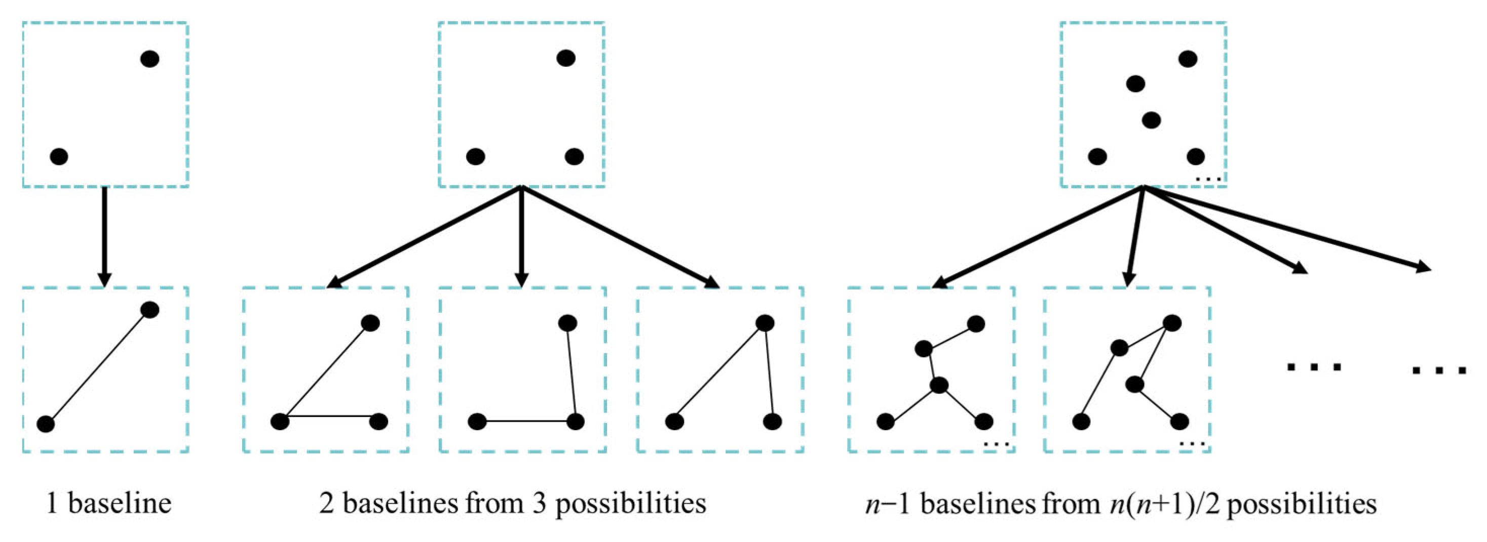
7]. The principle of independent baseline selection is that only one path exists between any two stations, while all the stations should be connected. For a network with
n stations, a total of
baselines exist, only
of which are independent. The objective of the independent baseline selection is to optimize the overall accuracy of the baseline solutions in order to facilitate the subsequent network adjustment. Mathematically, this process can be described by the minimum spanning tree (MST) [
10,
11] problem.
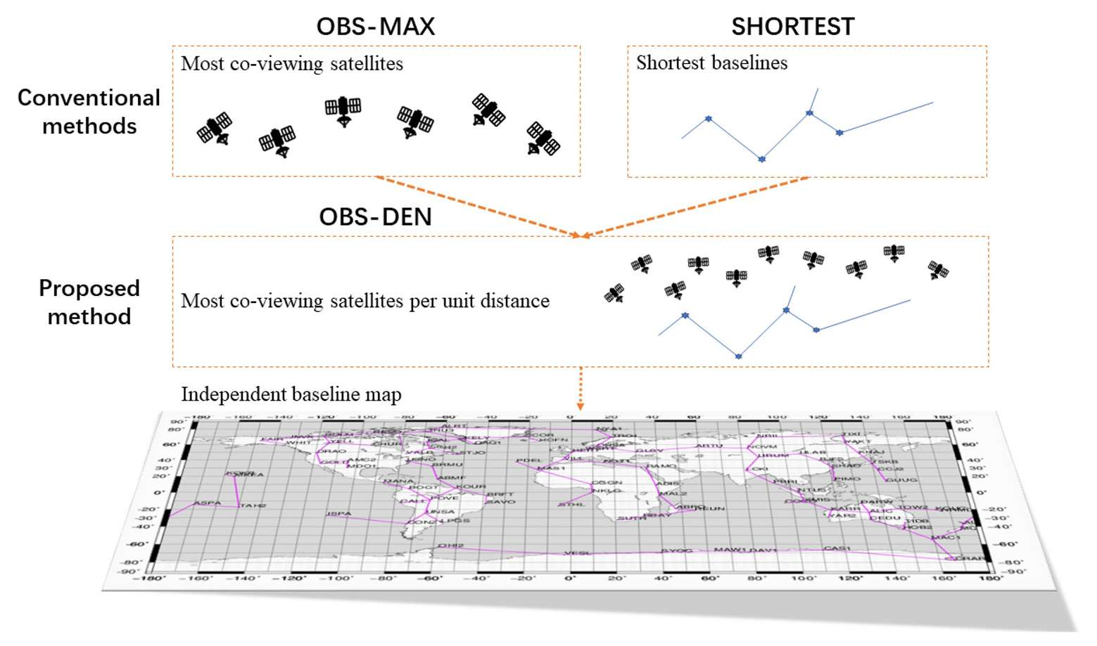
In the process of MST, the criteria for selecting baselines can be defined according to the user’s needs. One of the most easily conceived solutions is to make the total length of
baselines the shortest, which is known as the shortest path (SHORTEST) method [
7,
8]. This is because the shorter the distance between stations, the greater the number of co-viewing satellites, thus more redundant observations are involved to facilitate the network adjustment. More importantly, the tropospheric and ionospheric delays of neighboring stations are similar. The shorter baselines help to better eliminate these errors. Since the original intention of SHORTEST is to improve positioning accuracy by increasing the number of co-viewing satellites, a more straightforward solution is to use the maximum common satellites as the criterion. This method is known as the maximum observation method (OBS-MAX) [
8].
Both methods mentioned above have been investigated; for example, SHORTEST was used in a massive GNSS network of more than 2000 globally distributed stations [
12], while OBS-MAX is shown to be beneficial in the tropospheric delay estimation [
13]. In the ideal situation, the shorter the baseline, the more common observations there are. Then, SHORTEST and OBS-MAX should be fully equivalent. However, the statistics show that they are not consistent [
14], i.e., on various days, the baselines generated by different methods could ultimately lead to different solution precision, which violates the assumption that the two methods are equivalent. This means that the number of observations does not necessarily increase as the baseline becomes shorter. This is due to the fact that the satellites are usually not evenly distributed across the sky, e.g., sparse observations in local areas and sufficient co-viewing satellites for some long baselines. In a word, the search for optimal independent baselines is still an open question to be further investigated.
A scheme of setting up weights (WEIGHT) between SHORTEST and OBS-MAX has been proposed [
14]. The WEIGHT method was demonstrated to be of higher positioning precision than that of SHORTEST and OBS-MAX. However, how to set up weights lacks theoretical support and can only be empirical. For instance, the weights can be determined based on the posterior accuracy of the final baseline solutions using each of the two methods; on an a priori basis, the Bernese software could use a weight of 30% for the SHORTEST in addition to OBS-MAX as an option [
8].
To avoid setting up empirical weights or doubling the computational load brought by a posteriori precision-based weighting, a new method called “observation-density” (OBS-DEN) is proposed here. It takes the ratio of baseline length and the number of observations between two stations as the criterion of the MST. The physical interpretation of this criterion is the number of common satellites per unit distance, which overcomes the degradation of baseline accuracy by seeking only maximum observations or the shortest baselines. The advantage of OBS-DEN is that it provides an explainable weighting scheme that can overcome the downsides of SHORTEST and OBS-MAX. This method can be used in various types of GNSS network solution-related software, alongside existing options for users to choose from.
The rest of the paper is organized as follows. In
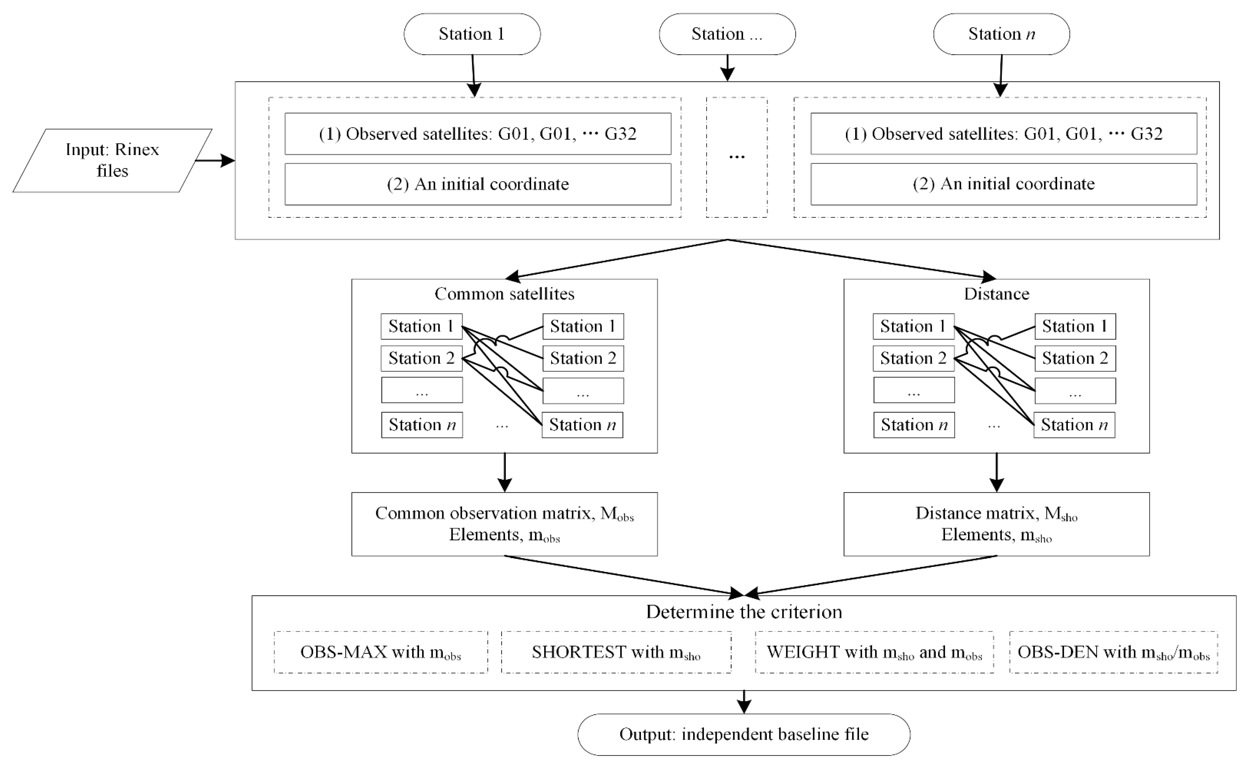
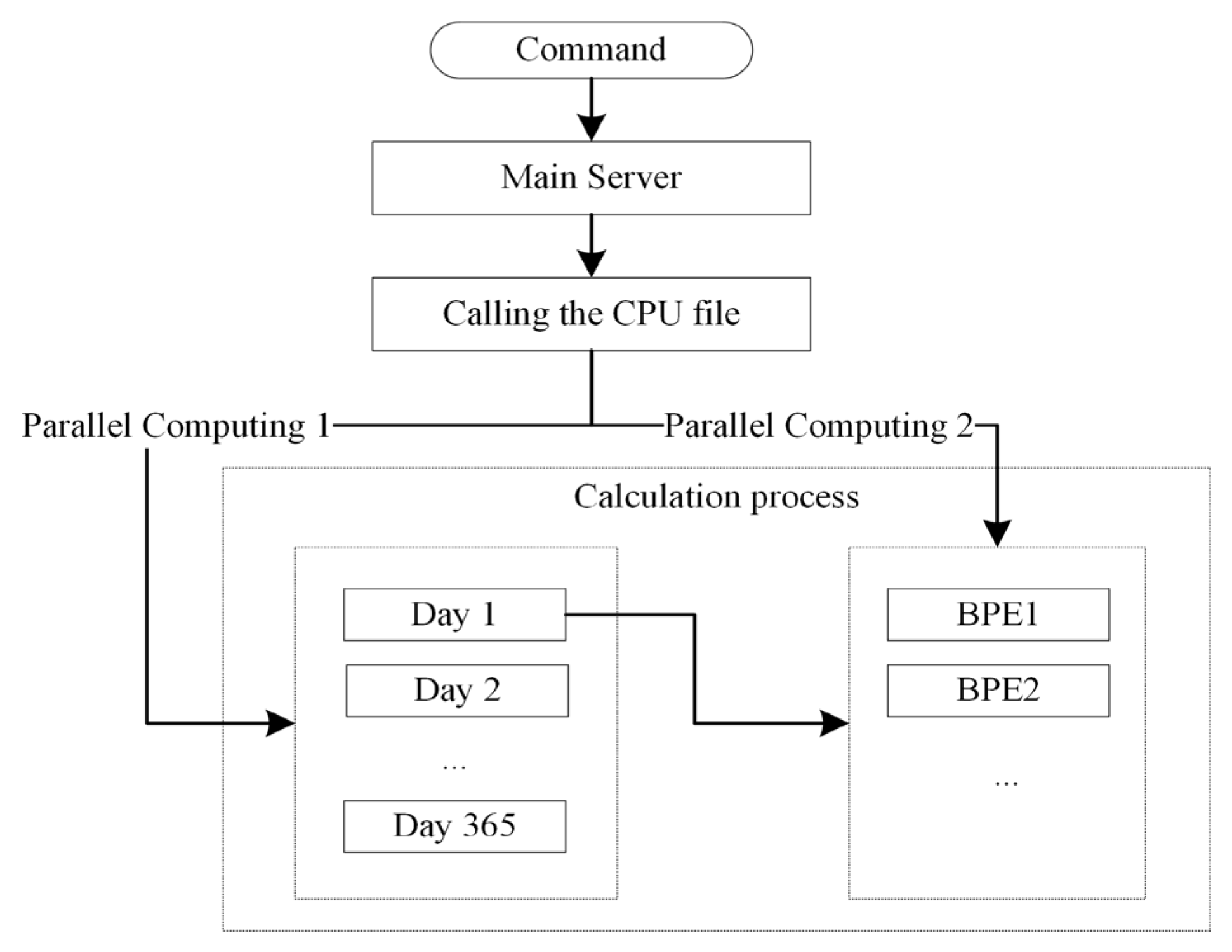
Section 2, the datasets and products, the principle of MST, and the criterion with OBS-DEN are introduced. Then the flowchart for generating independent baselines using various methods and the parallelization of network processing is presented in
Section 3. Afterward, the results of single-day solutions and annual statistics are analyzed and discussed in
Section 4. Finally, the paper is concluded in
Section 5.
3. Results
This section first shows the results of a single-day solution, including a comparison of the precision of the different methods, and the generated baseline map for our proposed method. The number of observations versus baseline length is also analyzed. After that, statistical results for one year using different methods are shown.
3.1. Single-Day Solution
At first, an experiment was conducted using globally distributed stations on 13 January 2012. The GNSS network solution was performed in the ITRF08 (International Terrestrial Reference Frame 2008). After the network adjustment, the results were converted to the local ENU (East-North-Up) coordinate system using the final coordinate products in SINEX format (Solution Independent Exchange Format) provided by CODE (Center for Orbit Determination in Europe) as a reference.
As is shown in
Table 1, OBS-DEN has the smallest 3D RMS error of 7.30 mm, followed by SHORTEST. For SHORTEST, the large error in the E direction drags down its RMS. Compared with the commonly used OBS-MAX and SHORTEST, OBS-DEN has mainly improved the East and North accuracies.
STD represents the degree of dispersion of the error for all stations. Although OBS-DEN has the lowest 3D RMS error, it has a larger STD compared to SHORTEST in the U direction. The STD of N and U components of OBS-MAX are the largest, which indicates that some individual stations may have large errors with OBS-MAX. Generally, it can be seen that the positioning errors of OBS-DEN are less discrete compared to other approaches.
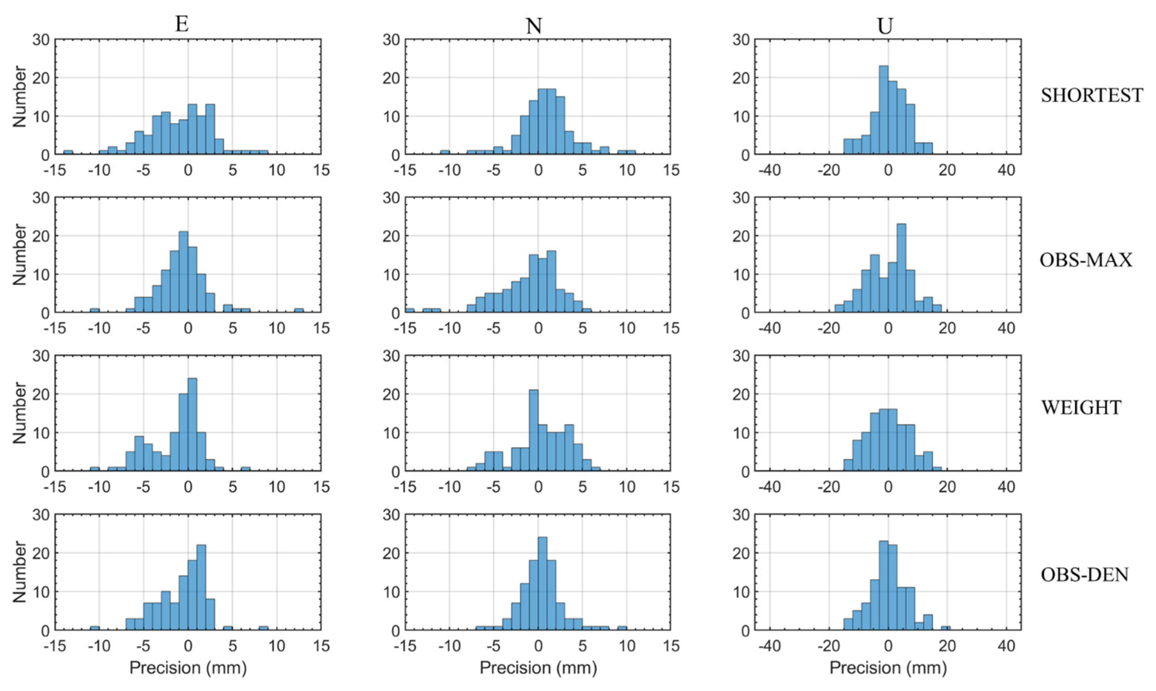
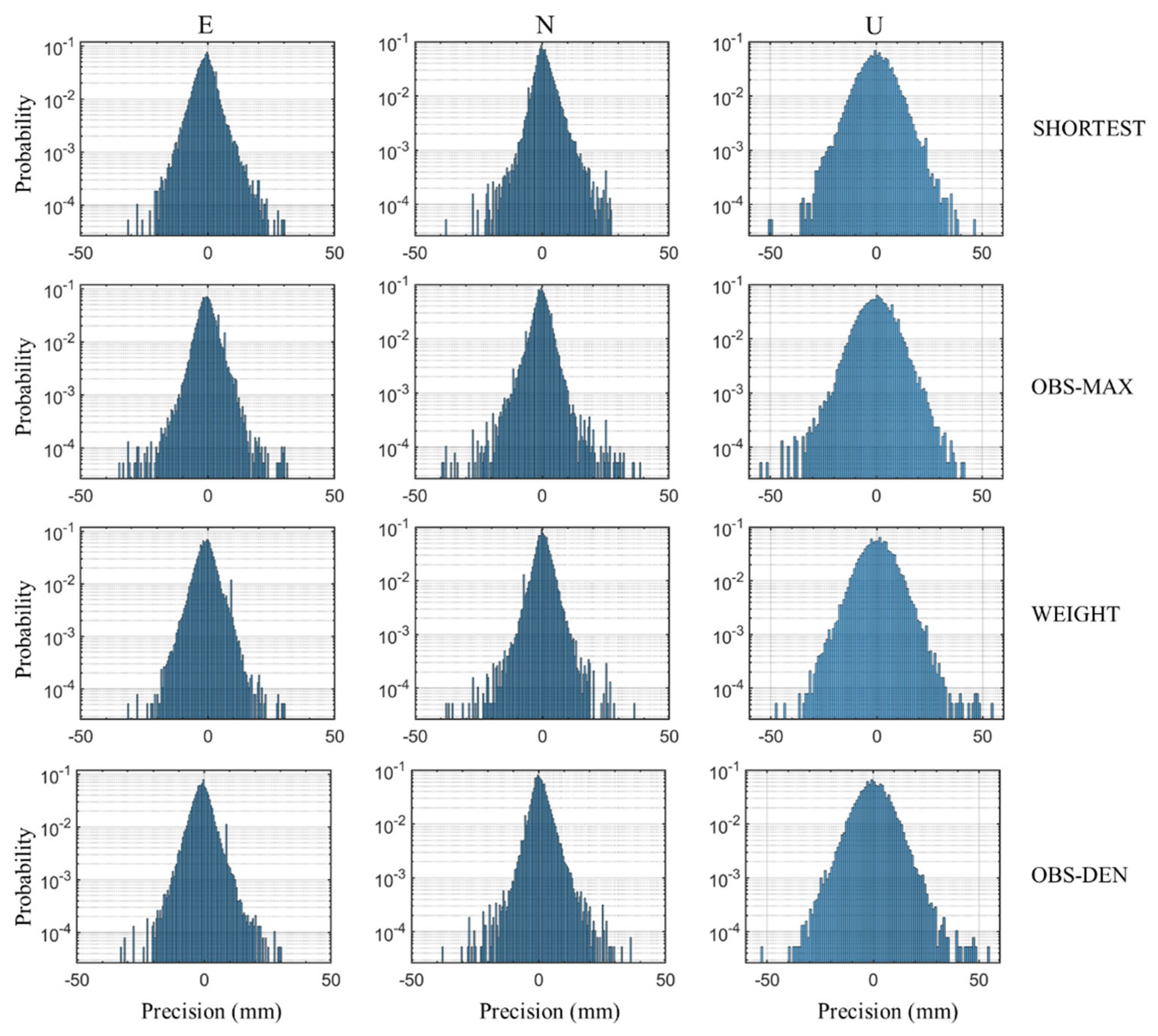
Histograms of the single-day solution showing the coordinate error distributions in the E, N, and U directions of different methods are presented in
Figure 4. In the East direction, the error distribution of OBS-DEN is closest to 0 and has rare discrete bars (> 10 mm), followed by OBS-MAX; the center of the error distribution of WEIGHT deviates from 0 at about −1.4 mm, and there are agminated bars around −5 mm, which makes its precision worse than OBS-DEN and OBS-MAX in East. In the N direction, the errors of OBS-DEN are more concentrated, while OBS-MAX has the most discrete values. For the U component, the results of the various methods are broadly similar, with the errors of OBS-MAX being slightly dispersed.
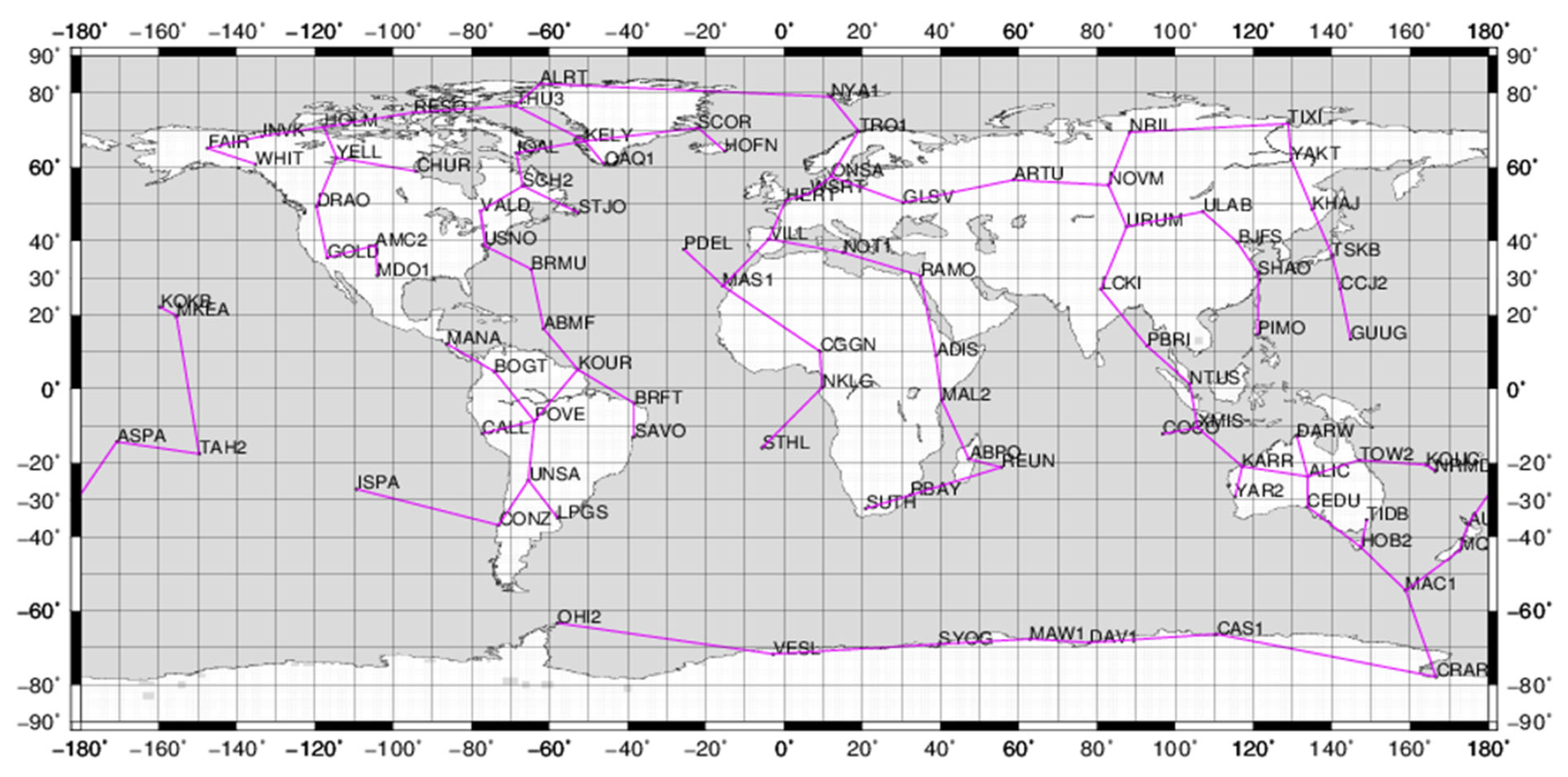
Figure 5 shows the baseline map of OBS-DEN. Since OBS-MAX emphasizes more DD observations, a ‘STAR’-like shape, i.e., a central station with plenty of observations connected with multiple nearby stations [
24,
25], will exist in many regions. For example, some stations in South America, Australia, and Europe shown in [
14] could connect more than 5 baselines. SHORTEST, on the other hand, has fewer baselines clustered towards the central stations, i.e., most stations are connected to only two or three baselines. As a result of a combination of the above two methods, some of the central stations of OBS-DEN, such as POVE in South America and ALIC in Australia, are connected to four baselines, while other stations are mostly connected to two or three baselines.
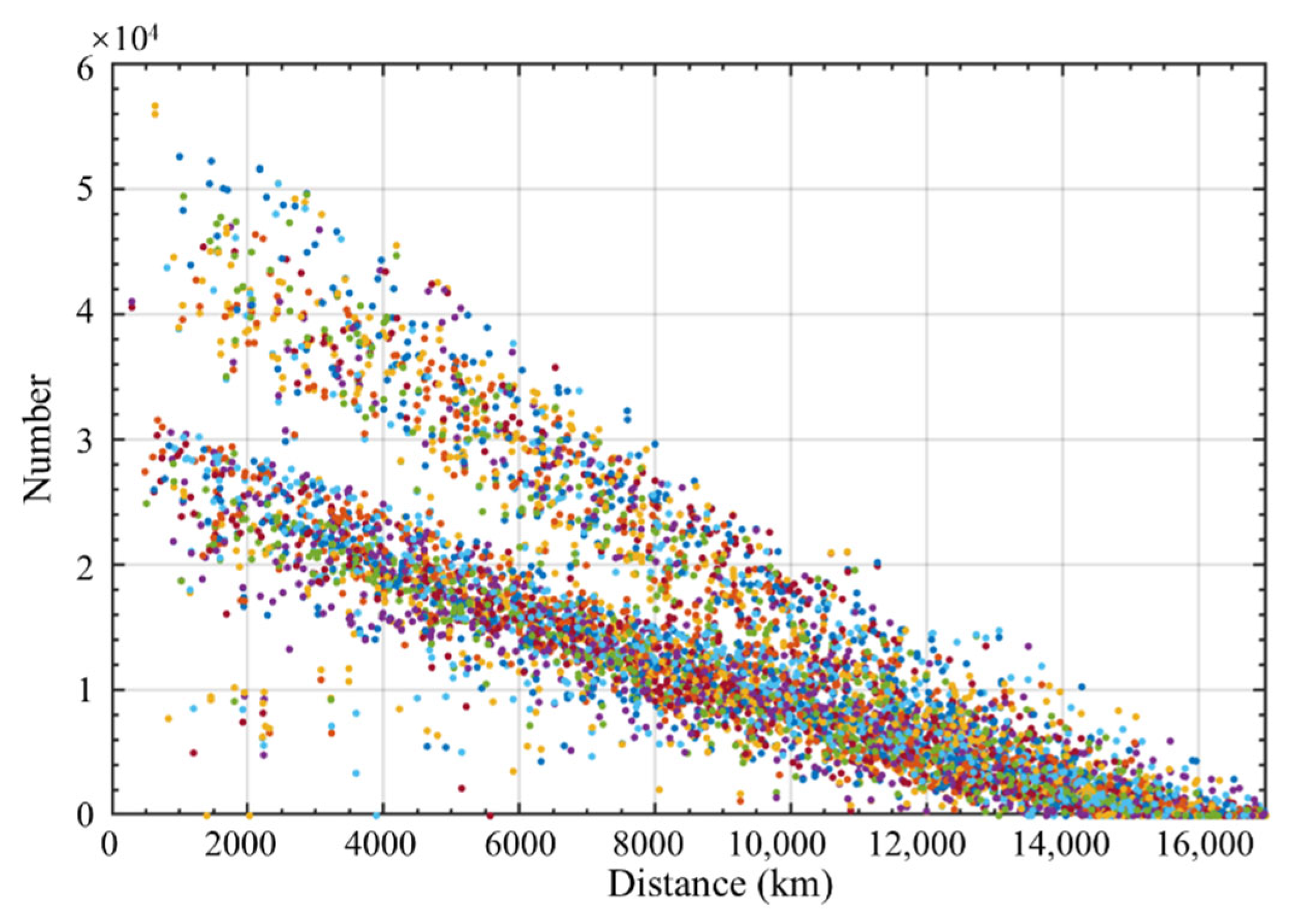
The number of DD observations versus the baseline length of each baseline is plotted in
Figure 6. It can be seen that the co-viewing satellites decrease roughly linearly with increasing distance. When the station spacing is greater than 17,000 km, the co-viewing satellites are almost absent. However, at distances of several thousand kilometers, there are still large numbers of common observations between stations. It is obvious that the baseline selection dominated by the number of DD observations, which is applied in OBS-MAX, is no longer applicable at this point. This is due to the long distances resulting in different tropospheric and ionospheric conditions, especially the baselines from mid-latitude to low-latitude/equatorial regions.
In the data analysis, we found that some stations have both GPS and GLONASS observations while others can receive only GPS signals. That is why there are two linear aggregations presented in
Figure 6. In addition to the two obvious linear aggregations, one can see some scattered dots to the lower left. These dots indicate that although the stations are close to each other, there are not many common observations. This may be due to a long-time loss of signal lock or bad observations being excluded. In this case, the baselines are short but with fewer observations. Thus, the SHORTEST method can possibly degrade the accuracy of the baseline solutions due to the introduction of these stations with a small number of observations, while OBS-DEN would avoid such baselines and instead choose baselines with sufficient satellites, but which are slightly longer, i.e., those from the upper-left region of
Figure 6.
3.2. One-Year Statistical Results
To better evaluate the performance of various methods, we have tabulated the statistical results for a year. The RMS errors in each direction and the distribution are summarized in
Table 2 and
Figure 7. Generally, the RMS and the distribution of the methods are comparable. In more detail, the probabilities that 3D errors exceed
ε, 2
ε, and 3
ε mm are presented, respectively, in the right column of
Table 2. The threshold ε is set as 9.67 mm, which is the average 3D RMS value of the four methods. From the statistical results, we can see that OBS-DEN has the most stations with accuracies within one
ε, and WEIGHT the least. However, the probability that WEIGHT is larger than 2
ε and 3
ε is the smallest. That is, the coordinate errors of WEIGHT lie more in the interval from
ε to 3
ε. OBS-DEN and OBS-MAX have more 3D errors larger than 3
ε, which pulls down the performance of OBS-DEN and OBS-MAX somewhat.
In addition to the tails of the distributions explored on the right side of
Table 2, the histograms showing the coordinate error distributions can be seen in
Figure 7. Overall, the distribution of the four methods is similar. However, SHORTEST has fewer burrs for errors greater than 30 mm, especially in the North direction. The distributions of the four methods in the East direction seem to be a little fatter than that in the North, which shows that the STD is minimal in N. For the Up direction, there are large discrete errors around or larger than 50 mm for all four methods.
4. Discussion
Overall, OBS-DEN achieves the desired precision in terms of the RMS 3D of station coordinates and shows its capability to get comparable or even better precision than other methods. OBS-MAX is overly focused on the number of observations, but it may include some long baselines with low precision, while SHORTEST is excessively focused on baselines’ length and may have incorporated some short baselines with less co-viewed satellites. OBS-DEN excludes these two extreme conditions by both pursuing high observation numbers and also emphasizing short baselines. When compared with WEIGHT, although the accuracy improvement of OBS-DEN is limited, it provides a rational option rather than determining weights empirically.
In theory, with the same information obtained, the final results should be equivalent, but the different ways of data processing led to inconsistent information or data involved. The advantage of OBS-MAX is that it absorbs more redundant observations involved in the adjustment. However, from the above results, especially in
Figure 6, there are still a considerable number of observations at a certain range with baselines getting too long. In this case, OBS-MAX may pick some long baselines and make the results worse. In addition to the impacts of the tropospheric and ionospheric delays, the DD ambiguity is more difficult to deal with when the baseline becomes longer [
26]. The advantage of SHORTEST is that it uses stations from short baselines whose atmospheric delays are basically the same. However, the shortest baseline could not necessarily exclude the baselines with few co-viewing satellites. As a synthesis of the above two methods, the ratio of the baseline length to the number of observations can be used to overcome the respective shortcomings of the previous individual methods, resulting in a better baseline solution in certain scenarios.
In addition to these most common methods, there are the maximum-ambiguity-fixed-rate method [
27] and the STAR method [
8]. However, the former uses the outcome of the solution as a basis for selection and cannot provide a pre-defined option for the independent baseline solution as other methods. The STAR method is commonly used for local networks rather than global ones. Therefore, only OBS-MAX and SHORTEST from the traditional methods are involved in the comparison. In future work, the performance of different constellations including positioning accuracy, number of observations, and signal quality could also be used as another baseline searching criteria.
The baseline solution precision is closely related to the station location and density, the shape of the network, and the local atmospheric environment. Different baseline search strategies can be adapted to specific situations. For example, baseline solutions at low latitudes, equatorial and polar regions are usually affected more heavily by ionospheric effects [
28,
29], especially during a solar maximum period. Thus, more consideration should be given to making the baselines shorter during such periods.
It should be noted that the stations selected for this experiment are globally distributed. The results of these methods may be less different in a local area network where all stations have comparable observations. For example, for a local area network [
6] or network RTK (Real-Time Kinetic) [
30,
31,
32], the different baseline selection methods are theoretically close to being equivalent, especially with a large number of observations of multiple systems [
33]. While all stations are close to each other, the number of co-viewing satellites between them is also similar. The baselines selected by different methods may differ from each other, but the total length of the baseline and the total number of satellite observations will not vary significantly.
5. Conclusions
In light of the limitations of current independent baseline selection methods, such as OBS-MAX and SHORTEST, an alternative optimized scheme named OBS-DEN is proposed for GNSS network solutions. It is characterized by maximum co-viewing satellites per unit distance. Since the SHORTEST pursues only short baselines, there is a risk of introducing low-precision baselines with small co-observations numbers; OBS-MAX aims only for more observations and will potentially introduce baselines with large tropospheric and ionospheric differences. OBS-DEN considers both shorter paths and more DD observations in an independent baseline network. It compensates for the shortcomings of SHORTEST and OBS-MAX and does not require empirical weighting. It can be a new independent baseline search strategy for baseline selection in GNSS software, e.g., Bernese.
In both the single-day and annual solutions, OBS-DEN demonstrates its ability to obtain comparable or even higher 3D accuracies. In the single-day solution, the distribution of OBS-DEN is more concentrated. The RMS is smaller than OBS-MAX and SHORTEST. In the statistical results of annual solutions, the 3D RMS of OBS-DEN has the highest probability to be less than 9.67 mm, i.e., the average 3D RMS of all the four methods, compared to other methods.
Due to the uncertainty of the error distribution, OBS-DEN would not be better than other methods in all cases. Different network types and application scenarios correspond to different optimal baseline schemes. In scenarios where the traditional methods are both limited, OBS-DEN can be considered as the preferred scheme.


