Abstract
Hyperspectral images (HSIs) contain spatially structured information and pixel-level sequential spectral attributes. The continuous spectral features contain hundreds of wavelength bands and the differences between spectra are essential for achieving fine-grained classification. Due to the limited receptive field of backbone networks, convolutional neural networks (CNNs)-based HSI classification methods show limitations in modeling spectral-wise long-range dependencies with fixed kernel size and a limited number of layers. Recently, the self-attention mechanism of transformer framework is introduced to compensate for the limitations of CNNs and to mine the long-term dependencies of spectral signatures. Therefore, many joint CNN and Transformer architectures for HSI classification have been proposed to obtain the merits of both networks. However, these architectures make it difficult to capture spatial–spectral correlation and CNNs distort the continuous nature of the spectral signature because of the over-focus on spatial information, which means that the transformer can easily encounter bottlenecks in modeling spectral-wise similarity and long-range dependencies. To address this problem, we propose a neighborhood enhancement hybrid transformer (NEHT) network. In particular, a simple 2D convolution module is adopted to achieve dimensionality reduction while minimizing the distortion of the original spectral distribution by stacked CNNs. Then, we extract group-wise spatial–spectral features in a parallel design to enhance the representation capability of each token. Furthermore, a feature fusion strategy is introduced to increase subtle discrepancies of spectra. Finally, the self-attention of transformer is employed to mine the long-term dependencies between the enhanced feature sequences. Extensive experiments are performed on three well-known datasets and the proposed NEHT network shows superiority over state-of-the-art (SOTA) methods. Specifically, our proposed method outperforms the SOTA method by 0.46%, 1.05% and 0.75% on average in overall accuracy, average accuracy and kappa coefficient metrics.
1. Introduction
Hyperspectral images (HSIs) are captured by space-borne or airborne imaging spectrometers. Different from ordinary three channels (e.g., Red, Green, Blue) optical images, each pixel of HSIs contains a large number of dense and continuous spectral information in the channel dimension. The spectra of different objects contain unique spectral features, just like fingerprints [1], nd the subtle spectral discrepancies (discrepancies along the spectral dimension are considered as part of the spectral series information) of different targets is an important basis for achieving fine-grained classification. The purpose of HSI classification is to define a definite category for each pixel which provides information guidance for land change detection, object detection, precision agriculture and other earth observation missions [2,3,4].
Traditional machine learning methods of HSI classification, such as support vector machine (SVM) [5], dynamic subspace [6] and logistics regression [7] rely on the spectral information of pixels. These methods find it difficult to achieve accurate classification when the spectral variability is serious and abundant mixed pixels exist.
In recent years, CNN-based image classification algorithms stand out in the field of HSI classification [1]. For example, Chen et al. [8] discussed the influence of different CNN-based structures on feature extraction performance. Due to the strip distributed receptive field of 1D kernel, 1D CNNs are often known as spectral-based feature extractors. In [9,10], a 1D convolution kernel with a finite number of layers was used to extract spectral features directly. Hu et al. [11] employed stacked 1D convolution architecture to extract spectral features at multiple layers, and then the pixels were classified by fully connected layer. The 2D and 3D kernel-based backbone networks and their hybrid variants are regarded as spatial–spectral feature extractors. Lee and Kwon [12] combined multi-scale spatial–spectral features extracted by 2D and 3D CNNs. In order to prevent the gradient vanishing phenomenon caused by deep-stacked CNNs, the residual connection of ResNet [13] was introduced in HSI classification. Paoletti et al. [14] fused CapsNet and ResNet to achieve fast HSI classification. Zhong et al. [15] used a series of 3D kernels to extract spatial–spectral features jointly and the residual connection was used to enhance the interaction of deep and shallow features. Although the CNN-based methods have achieved remarkable classification performance, the entire network lacks flexibility after being designed. Due to its fixed kernel size and the limited number of layers, the backbone of CNNs shows limitations in capturing global information, especially in the spectral dimension of HSIs.
Recently, transformer network has shown a powerful ability to extract long-term dependencies of sequence data in the field of natural language processing (NLP) [16]. Different from CNN-based models, transformer has a global receptive field even in the shallow layer because of the self-attention mechanism. Some researchers applied transformer to HSI classification because the self-attention mechanism can be used to efficiently model the long-range inter-spectra dependencies. For example, He et al. [17] first used the transformer-based BERT [18] model for HSI classification. Hong et al. [2] proposed a pure Vision Transformer (ViT) [19]-based framework named SpectralFormer, which can learn locally detailed spectral representations by group-wise spectral embedding operation. In addition, this method applied the idea of skip connection to enhance the representation ability of tokens from shallow to deep. Qing et al. [20] adopted average pooling and maximum pooling operations as a spectral attention block to enhance the feature representation ability without losing spectral information. Then, the obtained feature maps were fed into transformer for classification. These pure transformer-based methods effectively model the long-range dependencies of spectra; however, they often divide the entire HSI patch into a series of tokens which prevent the transformer from efficiently modeling spatial contextual information.
In order to improve the spatial information representation capability of tokens, some approaches combine the CNNs (e.g., VGGNet [21], ResNet [13], etc.) with the transformer model. The CNN-based backbones are firstly used to extract the locally spatial context information of the hyperspectral data. Then the feature maps output from the CNNs are transformed into sequential features (tokens) and sent to the transformer to further model the deep inter-spectral dependencies. We refer to this as two-stage approach. For example, He et al. [22] combined VGGNet with transformer and used the pre-trained VGGNet as the teacher network to guide the VGG-like model to learn the spatial features of HSIs. Finally, the whole feature maps were fed into the transformer. In [23], Le et al. proposed a Spectral-Spatial Feature Tokenization Transformer (SSFTT). The SSFTT used principal component analysis (PCA) [24] and stacked hybrid CNNs to reduce the dimension of original HSI data and extracted spectral–spatial features, respectively. Then, the Gaussian distributed weighted tokenization module makes the features keep in line with the original samples which is beneficial for transformer to learn the spectral information. Yang et al. [25] proposed a CNN-based Hyperspectral Image Transformer (HiT) architecture and the Conv-Permutator of HiT was used to capture the information from different dimensions of HSI representations. Furthermore, other joint CNN and Transformer networks (i.e., LeViT [26], RvT [27]) were also applied to HSI classification to demonstrate the superiority of HiT.
The aforementioned joint CNN and Transformer architectures allow the model to further capture locally spatial context and reduce spatial semantic ambiguity in extracting spatially structured information from sequential features. However, these two-stage feature extraction methods are not effective in learning the spatial–spectral correlations of HSIs. In addition, CNNs overly focus on spatial information, which distorts the continuous nature of the original spectral signatures and increases the difficulty of the subsequent transformer to model the discrepancies of spectral properties. The classification accuracy of the two-stage methods is even lower than that of some multidimensional CNNs when the target to be classified has strong spectral intra-class variability or inter-class similarity.
In summary, the existing joint CNN and Transformer classification methods distort the sequence relationship of original spectral information in enhancing the spatial representation capability which further weakens the ability of the self-attention mechanism to distinguish subtle discrepancies of spectra. Aiming at the aforementioned limitations of current methods, we propose a Neighborhood Enhancement Hybrid Transformer (NEHT) network for HSI classification. The proposed network is roughly divided into three components: Channel Adjustment Module (CAM), Spectral Pooling and Enhancement Module (SPEM) and Hybrid Attention Module (HAM). First, we use a very simple CAM which includes a 2D convolution operation to extract the shallow features of the HSI. Second, to improve the spatial–spectral representation capability of tokens, we propose the SPEM module, which mainly contains two blocks, named the Spatial Neighborhood Enhancement (SANE) block and Spectral Neighborhood Enhancement (SENE) block. These two parallel-designed blocks can model the spatial and spectral relations simultaneously, further providing opportunities for extracting spatial–spectral features and achieving better feature representation learning. We also introduce a feature fusion strategy in SPEM that generates the complementary spatial–spectral clues of adjacent bands for each token, and enhances the transformer’s ability to identify subtle discrepancies between spectra for fine-grained classification. Finally, the HAM adopts the self-attention mechanism of transformer to capture the global correlation between the enhanced tokens and gives the classification results.
The main contributions of this paper is listed as follows:
1. Compared to the existing method of stacking CNNs before the transformer, which applies the shared weights to all bands, an efficient parallel-designed CNN-based structure named SPEM is proposed in NEHT network for extracting reliable spatial–spectral features from neighbor bands. The two blocks contained in SPEM can generate the data-dependent weights that enhance the generalization capability of the model.
2. To minimize the distortion of the continuous nature of spectral signature by stacked CNNs, a residual-like feature fusion strategy with Shift-and-Add Concatenation operation is proposed to enhance the distinguishability of spectra without losing the original fine features.
3. The special hybrid architecture enables the transformer to learn more reliable spatial–spectral information from shallow to deep. The experiments verify the superiority of the proposed method and the impact of some key parameters in the network are studied exhaustively.
2. Related Work
2.1. Joint CNNs with Transformer
Transformer-based methods have recently dominated a wide range of tasks in the field of computer vision since Vision Transformer (ViT) [19] achieved competitive performance in image classification. However, compared with CNNs, ViT shows limitations in extracting explicitly low-level edges and texture information, which are highly spatially correlated [28]. The reason for this is that the ViT adopts the sequence-based input while CNNs adopt image-based input. To address this issue, some researchers introduce the desirable properties of CNNs to transformer-based methods while maintaining the merits of both architectures. Here, we briefly review the joint CNNs with transformer model for vision tasks. Guo et al. [29] proposed a novel CNNs-meet-transformers (CMT) model. The CMT used standard convolution with a stride of two to reduce the size of the input image. Then, the CMT block combined depth-wise convolution with self-attention mechanism to introduce local information for transformer. Li et al. [30] brought locality to ViT by adding depth-wise convolution into the feed-forward network of transformer. The Conditional Position encodings Visual Transformer (CPVT) [31] adopted the Positional Encoding Generator (PEG) which is composed of depth-wise separable convolution to generate convolutional projection for transformer. The aforementioned methods try to integrate CNNs with transformer to break the bottleneck of a single model in the vision tasks.
2.2. Joint Model for HSI Classification
Hyperspectral images are considered to be special 3D image data cubes that are highly spatially and spectrally correlated. Inspired by the joint model, some methods use the joint model to capture the spatial–spectral information of HSIs. Specifically, CNNs are used to extract spatially structured information and transformer is used to model the long-range inter-spectra dependencies. For example, Wang et al. [32] proposed stacked CNN-based selective kernel architecture to extract spatial–spectral features between different receptive fields. Then, the ViT-based model with the re-attention mechanism was adopted to increase the diversity of attention maps at different levels. Yang et al. [33] applied CNN-based Conv-layer to form the local branch and used the CNN-transformer module to form the global branch. Finally, the features from the two branches were fused for the final classification. Dang et al. [34] proposed a spatial–spectral attention module which contains CNN and pooling operation to extract the low-level features for transformer. Xue et al. [35] adopted an auto-designed hybrid CNN-Transformer framework that could search optimal CNN architectures for transformer by the neural architecture search algorithm. Zhang et al. [36] integrated CNN-based auto-encoder with Mobile ViT to achieve lightweight HSI classification.
The above methods successfully enhance the ability of transformer in capturing locally spatial information by joint various stacked CNNs which use shared weights for total bands of HSI. However, they ignore the spatial–spectral correlation when extracting the spatial features. Meanwhile, the stacked CNNs distort the continuous nature of spectral signature which may blur the subtle discrepancies between the spectra. In contrast to these concurrent works, our well-designed CAM and SPEM can efficiently extract data-dependent spatial–spectral features and increase the distinguishability of spectra.
3. Method
Figure 1 shows the macro-structure of NEHT network. The entire network consists of three components, namely Channel Adjustment Module (CAM), Spectral Pooling and Enhancement Module (SPEM) and Hybrid Attention Module (HAM), where CAM and SPEM are CNN-based architectures and HAM is purely transformer-based architecture. Note that the grouping operation in CAM and the Shift-and-Add Concatenation (SAC) operation in SPEM are non-parametric operations.

Figure 1.
Overall architecture of the proposed NEHT network for HSIs classification. The NEHT network is composed of the Channel Adjustment Module (CAM) in the red rectangle, the Spectral Pooling and Enhancement Module (SPEM) in the green rectangle, and the Hybrid Attention Module (HAM) in the blue rectangle.
Firstly, each patch data from the original HSI is selected as input. Second, the CAM is used to reduce the dimensionality of each patch by standard 2D convolution and to group feature maps in the channel dimension. After that, two parallel designed blocks (i.e., SANE and SENE) are used to model the spatial–spectral correlations of each group feature map. Then, all groups from CAM will perform a feature fusion strategy with SAC operations to increase the subtle discrepancies between spectra. These operations are included in the SPEM. Finally, the feature maps output from SPEM is sent to HAM along the channel dimension to model the long-range inter-spectra dependencies and obtain classification results. In the following, we will illustrate three components in detail.
3.1. Channel Adjustment Module (CAM)
The data size of HSI cube in spectral domain is determined by imaging spectrometers. Some band selection algorithms can extract representative spectral features from hundreds of narrow bands, but it will inevitably lead to the loss of refined features. As the first part of the NEHT network, CAM uses only one layer of 2D convolution kernels, not complex CNNs with multiple layers to reduce the dimensionality of HSI; this simple operation mitigates the problem of distorting the inter-spectra dependencies of the original spectrum caused by the stacked CNNs. Meanwhile, the CAM will also candidate the feature maps to be enhanced by the SPEM with pre-defined group size. The architecture of CAM is shown in Figure 1 red rectangle. Supposed that the input of CAM is , where indicates the spatial patch size, B is the number of spectral bands from the original HSI cube. The calculation of channel adjustment is as follows:
where and are the output value at position and bias of the jth feature map in the ith layer, respectively. i, j and m are the index of convolution layer, feature map and the output feature map, respectively. is the weight at position for mth feature map and is the spatial size of convolution kernel. means the activation function. The final is the feature maps adjusted by the number of convolution kernels and is a subset of the total bands. Then, the CAM will group the output feature maps for the subsequent Spectral Pooling and Enhancement Module (SPEM) based on the preset grouping size. Taking neighborhood group size as g, the grouping formula is as follows:
where represents the kth feature map of y and is the kth selected group feature map.
3.2. Spectral Pooling and Enhancement Module (SPEM)
In this part, we propose the parallel-designed SPEM which can fuse adjacent bands and strengthen the spatial–spectral representation capability of tokens. The details of SPEM are described next.
3.2.1. Parallel Design of The SPEM
As shown in Figure 2, two blocks form the parallel branch in the SPEM. The left block represents Spatial Neighborhood Enhancement (SANE) block which contains standard Conv2D and batch normalization that can extract spatially contextual information from neighboring channels. The right block represents Spectral Neighborhood Enhancement (SENE) block which contains degraded Conv3D and batch normalization that is used to model the pixel-wise dependencies between neighboring bands. Furthermore, the activation function adopted in SPEM is the Relu function. Each block of SPEM adopts the idea of group convolution, which can generate group-dependent (subset of ) weights as done in dynamic networks [37,38]. Next, we present the designs of these two blocks in detail.
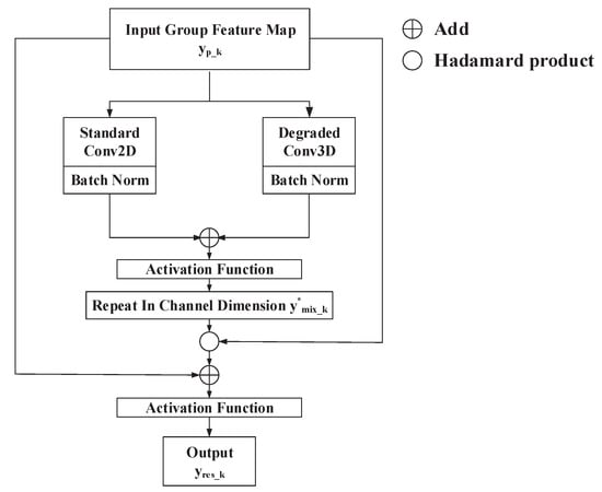
Figure 2.
The Flowchart of the Parallel Design of The SPEM.
Spatial Neighborhood Enhancement (SANE) Block: According to the excellent performance of 2D convolution kernel in modeling the local dependencies between nearby pixels, the SANE block also uses 2D kernels with the size of 3 × 3 to extract the spatial neighborhood features. The calculation is the same as the 2D convolution operation in Equation (3), where is the kth selected group feature maps from the output of CAM, ⊙ means the standard convolution operation and indicates the spatial enhancement feature map. and b indicate weight and bias, respectively.
Spectral Neighborhood Enhancement (SENE) Block: The 3D convolution kernel can focus on both spatial and spectral features of the target. However, using too large 3D convolution kernels or too many convolutional layers will cause redundancy of parameters and additional computational burden, that may lead to over-fitting. In SENE block, we use the degraded 3D convolution kernels (the kernel size is ) to capture the pixel-wise spectral features. Different from the general 3D convolution operation, the depth of the degraded 3D kernel is the same as the group size, so the filter slides only in two dimensions. This operation is written as:
where indicates the spectral enhancement feature map and is considered as a response peak mapping in a specific band range. are the position of feature map and are the position of weight. Other variables have the same definitions as those mentioned in Equation (1) and (3).
3.2.2. Feature Fusion Strategy
In spectral domain of HSI, the spectral response peaks of different categories may appear in different intervals with a fixed wavelength range which can well characterize the distinguishability of objects. When the target to be classified has very high spectral similarity, the spectral intervals containing subtle discrepancy will be extremely important for achieving fine-grained classification. However, this discrepancy often presents in the original spectral space and may be distorted by stacked CNNs. Based on the analysis above, to enhance the spectral discrepancy density and reduce the loss of detailed information, an effective feature fusion strategy is proposed.
Firstly, the feature maps obtained by two groups of enhancement blocks are added in the spatial dimension to obtain a mixed feature map (see Equation (5)), where and represent the kth spatial enhancement feature map and spectral enhancement feature map, respectively. indicates the position on the feature map.
Secondly, the mixed feature map is repeated in the channel dimension (becomes ) to keep its channel the same as the , and then linearly mapped to the corresponding grouping. The operation is as follows:
where are the index of feature map, k is the index of group and , means the selected kth grouping feature map and kth hybrid enhancement feature map, respectively. ∘ is Hadamard product. It is worth noting that the is the kth feature map of that expanded in channel dimension.
Thirdly, to alleviate the gradient-vanishing phenomenon, the residual connection is used to combine the feature maps from the output of CAM.
where , indicate the output of CAM and of SPEM, respectively. The final output is calculated by the following operations which we define as Shift-and-Add Concatenation (SAC). First, we define an intermediate variable , where and g represent the output channel of CAM and group size. The calculation of SAC is as Equation (8), any two adjacent and are arranged backward by one position in the row direction, then summed in the column direction and finally the resulting elements are concatenated in the channel dimension. The detail of the proposed CAM and SPEM is shown in Algorithm 1.
| Algorithm 1: The Operation of CAM and SPEM |
Input: Input an subset of HSI data , output channel of CAM ,and group size (g). Output:.
|
3.3. Hybrid Attention Module (HAM)
Previous works such as [28,39,40] show that by combining an efficient convolution module with a self-attention mechanism, one can obtain the merits of both of them.
Inspired by the preceding work, the HAM directly flattens the feature maps calculated by SPEM into sequential features and learns the long-term dependencies of deep spatial–spectral semantic information. It can be divided into the following three parts: Flatten Patch Layer, Encoder Block and Multi-Layer Perceptron (MLP) Head.
3.3.1. Flatten Patch Layer
Different from the patch embedding layer in the general ViT model, the input feature maps are directly divided according to the channel dimension. Each channel is regarded as an input patch and each input band is flattened into a hybrid token . This operation means that the spatial–spectral information from SPEM can be completely retained. It is well-known that the self-attention mechanism in transformer is capable to capture globally sequential information by the means of positional encoding [41]. To recover the permutation information of the original spectrum, we add additional learnable position embedding information and class embedding information for classification. The final output of the flatten patch layer is as follows:
where represents nth token and , are learnable parameters for class embedding and position embedding, respectively.
3.3.2. Encoder Block
The number of encoder blocks determines the depth of the entire ViT model. Each encoder includes layer normalization (LN) [42], multi-head self-attention (MHSA), and multilayer perceptron (MLP) block. We can see the residual connection is used in each encoder block. Since there are few HSI data available for training, drop path [43] mechanism is added in each encoder block to prevent over-fitting. The total encoder block is shown in Figure 1.
The first part of the encoder block is the LN layer which mainly normalizes the input sequence data to alleviate the internal covariate shift problem [44] and the data is projected to the nonlinear region of the activation function. The second part of the encoder block is MHSA, which is the core of the total transformer model. According to the Equations (9), the structure of input of the encoder block is the long-term sequential feature. To learn the global correlation between different tokens, the self-attention mechanism is introduced to our methods. For each input sequence , we use three linear mapping layers to obtain the mapping matrix , and of , respectively. The output of the attention mechanical is as follows:
where means the dimension of the matrix. If only one head is used, the framework of the attention mechanism is shown in Figure 3 (Left). Actually, there is more than one head for our HAM. MHSA is beneficial to extract deeper semantic information which is written as:
The structure of MHSA is shown in Figure 3 (Right). The relationship between classification performance and the number of heads will be discussed in the Section 4. The third part of the encoder block is MLP layer which contains two fully connected layers and a Gaussian error linear unit (GELU) [45] activation function.

Figure 3.
Architecture of attention mechanism. (Left) Self-attention. (Right) Multi-head self-attention [16].
3.3.3. Multilayer Perceptron (MLP) Head
The architecture of MLP head is similar to MLP layer, but the input of MLP head is the that we add in flatten patch layer. The final fully connected layer with softmax function is used as the classifier.
4. Results and Discussion
In this section, three well-known data sets are firstly described. Then, the implementation details of the network and environment configuration are introduced in the second part. Extensive experiments are conducted with ablation analysis to demonstrate the performance of our approach both quantitatively and qualitatively in the third part. Finally, other state-of-the-art methods are compared to show the superiority of our method.
4.1. Description of Data Sets
4.1.1. Pavia University Data Set
The Pavia data set was captured by the reflective optics system imaging spectrometer sensor (ROSIS). The Pavia University (PU) data set is a part of the Pavia data sets. It has a size of 610 × 340 pixels with a ground sampling distance of 1.3 m, and the spectral ranges from 0.43 to 0.86. After removing the noisy band, 103 bands are retained in the experiments. It has nine classes of interest that are annotated by different labels. The total number of labeled pixels is 42776, and the distribution of each category and its number is shown in the Table 1 below. Figure 4a shows the false-color version of the data set and its corresponding ground-truth label.

Table 1.
Land-Cover Classes of The Pavia University Data Set.
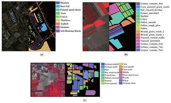
Figure 4.
The false-color maps and ground-truth maps of three data sets. (a) Pavia University data set, (b) Salinas data set, (c) Indian Pines data set.
4.1.2. Salinas Data Set
The Salinas (SA) data set was collected by the AVIRIS sensor over the Salinas Valley in Southern California. It has a size of 512 × 217 pixels with a ground sampling distance of 3.7 m. This data set has 204 spectral bands and 16 labeled categories. The false-color composite image and its ground-truth map are shown in Figure 4b. The number of pixels of each class is listed in Table 2.
Table 2.
Land-Cover Classes of The Salinas Data Set.
4.1.3. Indian Pines Data Set
The Indian Pines (IP) data set was also captured by the AVIRIS sensor which covers agricultural areas in northwestern Indiana. The spatial size of this data set is 145 × 145 with a ground sampling distance of 20 m. The false-color composite image and its ground-truth map are shown in Figure 4c. The number of spectral bands is 224 with wavelengths from 0.4 to 2.5. Because of the water absorption, 20 bands were removed, and only 200 bands were left. There are 16 classes in the 10,249 labeled pixels listed in Table 3.
Table 3.
Land-Cover Classes of The Indian Pines Data Set.
4.2. Experimental Configuration
We randomly divide the HSI cube into training, validation, and testing data sets represented by , , , respectively, and their corresponding label sets are denoted as , , , respectively. The is used to update network parameters which contain 5% of labeled data for PU and SA datasets and 10% for IP dataset. A total of 1% of the labeled data are used to verify the trained network. The entirety of the data are used for testing and calculating three evaluation metrics including Overall Accuracy (OA), Average Accuracy (AA) and Kappa Coefficient . In this article, the network is trained with 80 epochs for PU and SA data sets and 100 epochs for IP datasets. During the training procedure, Adam optimizer with the batch size of 64 is adopted, and the initial learning rate for PU and SA data sets are set as 0.005 and 0.0005 for IP dataset. We use the Multi-Step learning rate decay strategy: the decaying rate gamma is set as 0.1 for all data sets and the milestone is set as [20,40,80] for PU and SA datasets, and [60,80] for IP dataset. For different datasets, the input channel of CAM is determined by the number of spectral bands. The output channel of standard 2D convolution in CAM is 96 for the PU dataset and 196 for SA and IP datasets. The whole process is repeated five times to report the average accuracy. In every single epoch, the model configuration with the highest accuracy is used to evaluate the test set.
All the experiments have been operated on the hardware environment composed of an 8th-generation Intel R Core TM i7-8700 processor, with 12 MB of Cache and a processing speed of 3.20 GHz with 6 cores/12-way multi-task processing. The environment was completed with an NVIDIA GeForce GTX 1080Ti graphics processing unit (GPU) with 11 GB RAM. The software environment consists of the Windows10 pro 64-bit operating system with CUDA 10.1 and cuDNN 7.1 and Python 3.7 is the programming language. The network was built by pytorch 1.8. In order to alleviate data imbalance, we used inverse-median frequency to penalize the less frequently occurring classes more.
4.3. Parameter Analysis
To give a detailed and complete analysis of the proposed network, experiments are conducted for some key parameters of NEHT network in this section. The parameters include the patch size, the number of attention heads and encoder blocks, and the group size of CAM. Other parameters, such as batch size, learning rate and drop ratio, are fixed.
4.3.1. Evaluation the Influence of the Patch Size
In the data processing stage, the HSI cube needs to be divided into patches of the same size, and the label of each patch is determined by its center pixel. Each patch is flattened into an image sequence in the channel dimension before the attention mechanism. Dosovitskiy et al. [19] indicated that the size of each patch is inversely proportional to the length of the transformer, which means the FLOPS of transformer is similarly proportional to the depth and quadratic in width [46]. However, since the patch embedding layer is discarded in NEHT network, the width of transformer is directly determined by the output of CAM, and the output length for each data set is fixed. Intuitively, with the increase in patch size, the length of each sequence also increases and more parameters need to be learned. Therefore, patch size is positively correlated with the model complexity. Too large a patch size will make the network encounter an over-fitting problem. For searching the optimal patch size, we set it as , respectively, for three data sets.
Figure 5 presents the obtained results for PU, SA and IP data sets. The results illustrate that when the patch size is in the range , network performance is positively correlated with patch size. However, when the patch size exceeds , the OA scores tend to be flat or even slightly decline. Compared with PU and SA datasets, the IP dataset is more sensitive to changes in patch size. Finally, SA and IP data sets obtain the highest OA score at the patch size of , while for PU data sets, the maximum OA score appears at the patch size of .
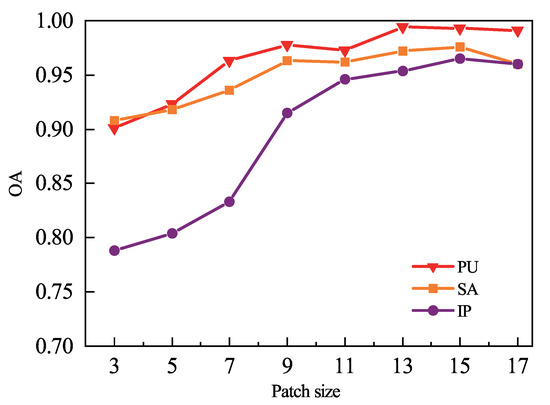
Figure 5.
OA of NEHT network with different patch size in the PU, SA and IP data sets.
4.3.2. Evaluation the Influence of the Attention Heads and Model Depth
The multi-head self-attention mechanism makes the transformer well modeling the dependencies between tokens. Increasing the number of heads is similar to increasing the number of feature maps in convolution and increasing the number of encoder blocks improves the model’s ability to extract deep semantic information. For the HSI classification task, the working dimension (i.e., model width) of the NEHT network and other transformer-based architecture is relatively fixed. The number of head and encoder block both determine the performance of the model. With limited training samples, an ultra-deep network will not only increase the computational complexity, but also degrade the network performance. Some transformer-based HSI classification methods separate the number of encoders and heads during the parameter analysis. We deem that adjusting the two parameters jointly is more beneficial to obtain optimal results.
We conducted experiments on different numbers of heads under different encoder blocks to dynamically measure the model depth that is most suitable for HSI data. We set the number of encoder blocks as 1, 2, 3, 4 and 5, respectively, at each depth we set the number of heads to 1, 2, 4, 8 and 16, respectively. The experimental results are shown in Figure 6. It can be concluded that the performance of the network gradually improves as the depth of the network increases, but when the depth is greater than 4, the performance starts to decline. For the three data sets, the highest OA scores are obtained when the model depth is 4 and the number of heads is 16.
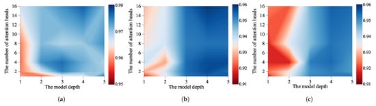
Figure 6.
The heat maps show the effect of dynamically adjusting the encoder blocks and attention heads of the network on OA of three data sets. (a) PU data set, (b) SA data set, (c) IP data set.
4.3.3. Evaluation of the Influence of the Group Size
For different categories, the distribution range of effective spatial and spectral features may be different. As the most important parameter in the SPEM, group size determines the distribution range of the fused feature maps, which improves the network’s ability to capture long-term dependencies and the semantic expression ability of tokens without directly increasing the width and depth of the model. Especially in the spectral dimension, different objects captured by the same sensor have different strong response intervals. For the targets with high interclass similarity, we need to pay more attention to the differences in spectral information in a certain wavelength range.
In order to find an optimal group size, we verify the classification effect of the model under different group sizes: 3, 5, 7, 9, 11 and 13. Figure 7 shows the effects of different group sizes on the classification accuracy of three datasets. According to the results, for PU and IP data sets, the highest OA score occurs when the group size is 9, and for SA dataset is 11. We can draw a common conclusion that with the group size increases, the subtle spatial–spectral discrepancies of neighboring feature maps can be better modeled by SPEM. However, it should be noted that too large a group size will increase the model inference time and weaken the representation ability of neighborhood feature maps.
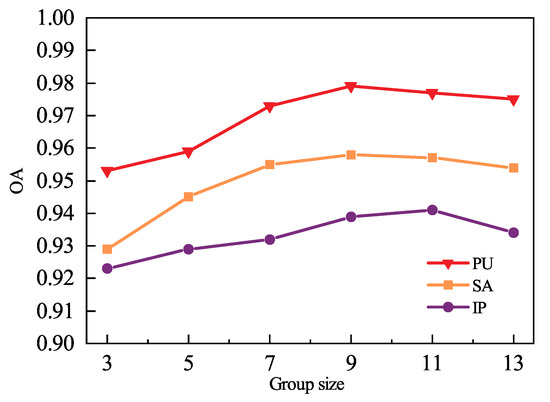
Figure 7.
OA of NEHT network with different group size in the PU, SA and IP data sets.
4.3.4. Ablation Analysis
To fully demonstrate the effectiveness of the proposed methods, we investigated the influence of different components that belong to the NEHT network on the IP data set. The whole model was divided into three components, and two of them need to be tested (i.e., CAM and SPEM). In addition, the SPEM is further divided into two blocks (i.e., SANE block and SENE block). The performance of each component and joint performance between different components are listed in Table 4. We also compare other stacked CNNs with transformer architecture to show the superiority of our proposed architecture for HSI classification tasks. The results are listed in Table 5.
Table 4.
Ablation Analysis of The Components on Indian Pines Data Set.
Table 5.
Ablation Analysis of The Proposed Method on Indian Pines Data Set.
In detail, the pure transformer-based method (ViT without CNN-based patch embedding module) yields the lowest classification accuracy, which means there are still many limitations of directly using the transformer for HSI classification. By adding either CAM or part of the SPEM into ViT, the classification accuracy has been improved. The fourth and fifth cases show that compared with CAM, SPEM can significantly improve classification accuracy (beyond 2.29% and 10.48% OAs, respectively). Comparing the second and third cases, without the channel adjustment module (CAM), spatial information is more effective for improving classification accuracy in the shallow layer of the network. Comparing the sixth and seventh cases, the CAM+SENE can obtain a higher OA score than CAM+SANE (0.34%), this may be that the combination of CAM and SENE extracts spatial and spectral information, while CAM+SANE pays more attention to spatial information. From the second, third, sixth and seventh cases, we can conclude that CAM can improve the reliability of features learned by any part of SPEM.
From Table 5, the joint stacked 2D or 3D CNN architectures with transformer do not bring a significant performance improvement. The hybrid convolution (2D+3D Conv) provides a more representative feature map for the transformer and obtains relatively better classification performance. Undoubtedly, the architecture that we proposed can further bring a performance improvement (more than 2% of OA, 5% of AA and 2% of ). In conclusion, the joint use of CAM and SPEM tends to obtain the highest classification accuracy.
4.4. Comparison with Other Methods
This section aims to compare the performance of the proposed NEHT network with some classical traditional methods, CNN-based deep learning methods, ViT-based method and joint CNN and Transformer methods. For the traditional methods, we chose SVM [5], random forest (RF) [47], multinomial logistic regression (MLR) [48] as the compared methods. For the CNN-based methods, PyResNet [14], ContextualNet [12], ResNet [13], and SSRN [15] were selected. For transformer-based methods, we took the pure ViT method as the baseline and the recent joint CNN and Transformer methods (i.e., SSFTT [23], LeViT [26], HiT [25]) as the comparison methods.
From Table 6, Table 7 and Table 8 we can conclude that our method outperforms other methods. Especially compared with the traditional methods, NEHT network appears more competitive. For the PU data set, the proposed NEHT network achieved 10.42%, 1.03% and 0.41% absolute improvement over the best traditional method, the CNN-based method and joint CNN and Transformer methods in the score of OA and achieved 14.44%, 0.83% and 0.57% absolute improvement in the score of AA. For the SA data set, the proposed NEHT network achieved 6.83%, 0.67% and 0.06% absolute improvement in the score of OA and achieved 14.44%, 0.28% and 0.27% absolute improvement in the score of AA, respectively. For the IP data set, the proposed NEHT network achieved 16.96%, 1.96% and 1.46% absolute improvement in the score of OA and achieved 21.43%, 1.38% and 2.3% absolute improvement in the score of AA, respectively. Figure 8, Figure 9 and Figure 10 present the comparison results of classification maps for different methods.
Table 6.
Classification Accuracy of Different Methods for Labeled Pixels of The PU Data Set.
Table 7.
Classification Accuracy of Different Methods for Labeled Pixels of The SA Data Set.
Table 8.
Classification Accuracy of Different Methods for Labeled Pixels of The IP Data Set.
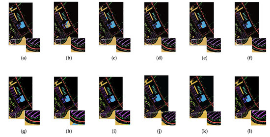
Figure 8.
Classification maps for PU data set. (a) SVM. (b) RF. (c) MLR. (d) ResNet. (e) PyResNet. (f) ContextualNet. (g) SSRN. (h) ViT. (i) SSFTT. (j) LeViT. (k) HiT. (l) NEHTNet.
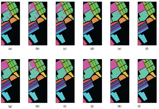
Figure 9.
Classification maps for SA data set. (a) SVM. (b) RF. (c) MLR. (d) ResNet. (e) PyResNet. (f) ContextualNet. (g) SSRN. (h) ViT. (i) SSFTT. (j) LeViT. (k) HiT. (l) NEHTNet.
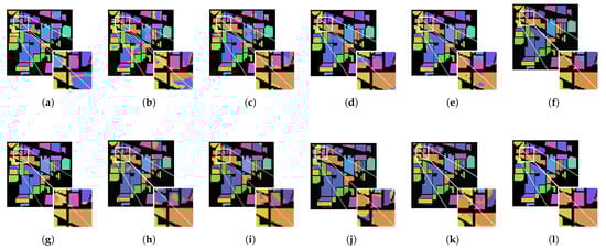
Figure 10.
Classification maps for IP data set. (a) SVM. (b) RF. (c) MLR. (d) ResNet. (e) PyResNet. (f) ContextualNet. (g) SSRN. (h) ViT. (i) SSFTT. (j) LeViT. (k) HiT. (l) NEHTNet.
We can observe that the traditional methods, especially those that only learn spectral features, show more misclassification of three considered data sets. Owing to the strong power of modeling locally contextual information, CNN-based methods obtain relative smooth classification maps, but they might lead to the misclassification of targets with small interclass distance. The pure ViT model without any CNN architecture does not achieve satisfactory classification results, because the self-attention mechanism is not as good as CNNs in fitting spatially structured information under limited training samples. We notice that the joint model obtains a higher OA score than CNN models. Although the gap between NEHTNet and SSFTT in OA scores is not large, our method is more robust in handling edge and texture details. This is because SPEM can extract highly semantic token representations from neighbor bands and increase subtle spectral discrepancies.
To evaluate how the training percentage affects the overall accuracy of the aforementioned methods, different numbers of training samples (i.e., 1%, 2%, 3%, 4% and 5% for PU and SA data sets and 2%, 4%, 6%, 8%, 10% for IP data) were selected. For samples whose total quantity does not meet the extraction ratio, we only take one pixel as the training set. Figure 11 gives the obtained results and it can be concluded that our method is superior to other methods with limited training data and shows more stable performance with fewer training samples (i.e., SA, IP data sets). When the portion of the training set increases, the gap in overall accuracy between the proposed method and other CNN-based methods becomes close. However, in the case of ultra-small training data for PU and SA data sets, the classification accuracy of SSFTT is slightly higher than that of our method, this may be because the traditional PCA dimensionality reduction algorithm used in SSFTT is more reliable than the data-driven deep learning algorithm.
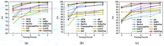
Figure 11.
OA(%) with different training rate with 1%, 2%, 3%, 4% and 5% for (a) PU and (b) SA data sets.2%, 4%, 6%, 8% and 10% for (c) IP data set.
5. Conclusions
In this paper, we propose a new joint CNN and Transformer network for HSI classification. The CNN-based CAM and SPEM are used to reduce the dimensionality of HSI and extract group-wise spatial–spectral features separately. The parallelly designed SPEM makes each token contain the spatial–spectral information of adjacent bands and provides diverse and shallow features for the transformer. Meanwhile, a feature fusion strategy is proposed to enhance the network’s capability to identify subtle discrepancies between spectra. Finally, the self-attention mechanism of transformer is used to model the long-term dependencies of tokens for achieving fine-grained classification tasks. The final experiment results demonstrate that the NEHT network achieves the highest accuracy compared to other methods in three data sets and exhibits robustness with small training samples.
In future work, we will investigate a lightweight joint CNN- and Transformer-based network to reduce the computational complexity without weakening the performance of the network. Furthermore, based on intuitive analysis, the larger the group size is, the more neighborhood spatial–spectral information it contains. However, with the increase in the group size, the performance of the model does not keep improving significantly. The main reason for this may be that the distribution range of strong response features of different targets is different, but we select a relatively optimal group size. In subsequent studies, we will try to introduce the idea of multi-scale group size to further improve the feature expression ability of neighborhood feature maps.
Author Contributions
Conceptualization, C.M. and J.J.; methodology, C.M. and H.L.; software, C.M.; validation, C.M., X.M. and C.B.; formal analysis, C.M. and X.M.; writing—original draft preparation, C.M., J.J. and X.M.; writing—review and editing, C.M. and J.J.; visualization, C.M., J.J., H.L., X.M. and C.B. All authors have read and agreed to the published version of the manuscript.
Funding
This research has received funding from the Youth Foundation for Defence Science and Technology Excellence(2017-JCJQ-ZQ-034).
Institutional Review Board Statement
Not applicable.
Data Availability Statement
Publicly available datasets were analyzed in this study, which can be found here: https://www.ehu.eus/ccwintco/index.php/Hyperspectral_Remote_Sensing_Scenes, accessed on 18 September 2022.
Conflicts of Interest
The authors declare no conflict of interest.
References
- Li, S.; Song, W.; Fang, L.; Chen, Y.; Ghamisi, P.; Benediktsson, J.A. Deep Learning for Hyperspectral Image Classification: An Overview. IEEE Trans. Geosci. Remote Sens. 2019, 57, 6690–6709. [Google Scholar] [CrossRef]
- Hong, D.; Han, Z.; Yao, J.; Gao, L.; Zhang, B.; Plaza, A.; Chanussot, J. SpectralFormer: Rethinking Hyperspectral Image Classification With Transformers. IEEE Trans. Geosci. Remote Sens. 2022, 60, 1–15. [Google Scholar] [CrossRef]
- He, L.; Li, J.; Liu, C.; Li, S. Recent Advances on Spectral–Spatial Hyperspectral Image Classification: An Overview and New Guidelines. IEEE Trans. Geosci. Remote Sens. 2018, 56, 1579–1597. [Google Scholar] [CrossRef]
- Camps-Valls, G.; Tuia, D.; Bruzzone, L.; Benediktsson, J.A. Advances in Hyperspectral Image Classification: Earth Monitoring with Statistical Learning Methods. IEEE Signal Process. Mag. 2014, 31, 45–54. [Google Scholar] [CrossRef]
- Melgani, F.; Bruzzone, L. Classification of hyperspectral remote sensing images with support vector machines. IEEE Trans. Geosci. Remote Sens. 2004, 42, 1778–1790. [Google Scholar] [CrossRef]
- Du, B.; Zhang, L. Target detection based on a dynamic subspace. Pattern Recognit. 2014, 47, 344–358. [Google Scholar] [CrossRef]
- Li, J.; Bioucas-Dias, J.M.; Plaza, A. Spectral–spatial hyperspectral image segmentation using subspace multinomial logistic regression and Markov random fields. IEEE Trans. Geosci. Remote Sens. 2011, 50, 809–823. [Google Scholar] [CrossRef]
- Chen, Y.; Jiang, H.; Li, C.; Jia, X.; Ghamisi, P. Deep feature extraction and classification of hyperspectral images based on convolutional neural networks. IEEE Trans. Geosci. Remote Sens. 2016, 54, 6232–6251. [Google Scholar] [CrossRef]
- Yang, X.; Ye, Y.; Li, X.; Lau, R.Y.; Zhang, X.; Huang, X. Hyperspectral image classification with deep learning models. IEEE Trans. Geosci. Remote Sens. 2018, 56, 5408–5423. [Google Scholar] [CrossRef]
- Haut, J.M.; Paoletti, M.E.; Plaza, J.; Li, J.; Plaza, A. Active learning with convolutional neural networks for hyperspectral image classification using a new bayesian approach. IEEE Trans. Geosci. Remote Sens. 2018, 56, 6440–6461. [Google Scholar] [CrossRef]
- Hu, W.; Huang, Y.; Wei, L.; Zhang, F.; Li, H. Deep convolutional neural networks for hyperspectral image classification. J. Sens. 2015, 2015, 258619. [Google Scholar] [CrossRef]
- Lee, H.; Kwon, H. Going deeper with contextual CNN for hyperspectral image classification. IEEE Trans. Image Process. 2017, 26, 4843–4855. [Google Scholar] [CrossRef] [PubMed]
- He, K.; Zhang, X.; Ren, S.; Sun, J. Deep residual learning for image recognition. In Proceedings of the IEEE Conference on Computer Vision and Pattern Recognition, Las Vegas, NV, USA, 27–30 June 2016; pp. 770–778. [Google Scholar]
- Paoletti, M.E.; Haut, J.M.; Fernandez-Beltran, R.; Plaza, J.; Plaza, A.J.; Pla, F. Deep pyramidal residual networks for spectral—Spatial hyperspectral image classification. IEEE Trans. Geosci. Remote Sens. 2018, 57, 740–754. [Google Scholar] [CrossRef]
- Zhong, Z.; Li, J.; Luo, Z.; Chapman, M. Spectral–spatial residual network for hyperspectral image classification: A 3-D deep learning framework. IEEE Trans. Geosci. Remote Sens. 2017, 56, 847–858. [Google Scholar] [CrossRef]
- Vaswani, A.; Shazeer, N.; Parmar, N.; Uszkoreit, J.; Jones, L.; Gomez, A.N.; Kaiser, L.; Polosukhin, I. Attention is all you need. Adv. Neural Inf. Process. Syst. 2017, 30. [Google Scholar] [CrossRef]
- He, J.; Zhao, L.; Yang, H.; Zhang, M.; Li, W. HSI-BERT: Hyperspectral image classification using the bidirectional encoder representation from transformers. IEEE Trans. Geosci. Remote Sens. 2019, 58, 165–178. [Google Scholar] [CrossRef]
- Devlin, J.; Chang, M.; Lee, K.; Toutanova, K. BERT: Pre-training of Deep Bidirectional Transformers for Language Understanding. arXiv 2018, arXiv:1810.04805. [Google Scholar]
- Dosovitskiy, A.; Beyer, L.; Kolesnikov, A.; Weissenborn, D.; Zhai, X.; Unterthiner, T.; Dehghani, M.; Minderer, M.; Heigold, G.; Gelly, S.; et al. An image is worth 16x16 words: Transformers for image recognition at scale. arXiv 2020, arXiv:2010.11929. [Google Scholar] [CrossRef]
- Qing, Y.; Liu, W.; Feng, L.; Gao, W. Improved Transformer Net for Hyperspectral Image Classification. Remote Sens. 2021, 13, 2216. [Google Scholar] [CrossRef]
- Simonyan, K.; Zisserman, A. Very deep convolutional networks for large-scale image recognition. arXiv 2014, arXiv:1409.1556. [Google Scholar]
- He, X.; Chen, Y.; Lin, Z. Spatial-Spectral Transformer for Hyperspectral Image Classification. Remote Sens. 2021, 13, 498. [Google Scholar] [CrossRef]
- Sun, L.; Zhao, G.; Zheng, Y.; Wu, Z. Spectral-Spatial Feature Tokenization Transformer for Hyperspectral Image Classification. IEEE Trans. Geosci. Remote Sens. 2022, 60, 1–14. [Google Scholar] [CrossRef]
- Licciardi, G.; Marpu, P.R.; Chanussot, J.; Benediktsson, J.A. Linear versus nonlinear PCA for the classification of hyperspectral data based on the extended morphological profiles. IEEE Geosci. Remote Sens. Lett. 2011, 9, 447–451. [Google Scholar] [CrossRef]
- Yang, X.; Cao, W.; Lu, Y.; Zhou, Y. Hyperspectral Image Transformer Classification Networks. IEEE Trans. Geosci. Remote Sens. 2022, 60, 1–15. [Google Scholar] [CrossRef]
- Graham, B.; El-Nouby, A.; Touvron, H.; Stock, P.; Joulin, A.; Jégou, H.; Douze, M. LeViT: A Vision Transformer in ConvNet’s Clothing for Faster Inference. In Proceedings of the IEEE/CVF International Conference on Computer Vision (ICCV), Montreal, BC, Canada, 10–17 October 2021; pp. 12259–12269. [Google Scholar]
- Heo, B.; Yun, S.; Han, D.; Chun, S.; Choe, J.; Oh, S.J. Rethinking Spatial Dimensions of Vision Transformers. In Proceedings of the IEEE/CVF International Conference on Computer Vision (ICCV), Montreal, BC, Canada, 10–17 October 2021; pp. 11936–11945. [Google Scholar]
- Wu, H.; Xiao, B.; Codella, N.; Liu, M.; Dai, X.; Yuan, L.; Zhang, L. Cvt: Introducing convolutions to vision transformers. In Proceedings of the IEEE/CVF International Conference on Computer Vision (ICCV), Montreal, BC, Canada, 10–17 October 2021; pp. 22–31. [Google Scholar] [CrossRef]
- Guo, J.; Han, K.; Wu, H.; Tang, Y.; Chen, X.; Wang, Y.; Xu, C. Cmt: Convolutional neural networks meet vision transformers. In Proceedings of the IEEE/CVF Conference on Computer Vision and Pattern Recognition, New Orleans, LA, USA, 21–24 June 2022; pp. 12175–12185. [Google Scholar]
- Li, Y.; Zhang, K.; Cao, J.; Timofte, R.; Van Gool, L. Localvit: Bringing locality to vision transformers. arXiv 2021, arXiv:2104.05707. [Google Scholar]
- Chu, X.; Tian, Z.; Zhang, B.; Wang, X.; Wei, X.; Xia, H.; Shen, C. Conditional positional encodings for vision transformers. arXiv 2021, arXiv:2102.10882. [Google Scholar]
- Wang, A.; Xing, S.; Zhao, Y.; Wu, H.; Iwahori, Y. A Hyperspectral Image Classification Method Based on Adaptive Spectral Spatial Kernel Combined with Improved Vision Transformer. Remote Sens. 2022, 14, 3705. [Google Scholar] [CrossRef]
- Yang, L.; Yang, Y.; Yang, J.; Zhao, N.; Wu, L.; Wang, L.; Wang, T. FusionNet: A Convolution–Transformer Fusion Network for Hyperspectral Image Classification. Remote Sens. 2022, 14, 4066. [Google Scholar] [CrossRef]
- Dang, L.; Weng, L.; Dong, W.; Li, S.; Hou, Y. Spectral-Spatial Attention Transformer with Dense Connection for Hyperspectral Image Classification. Comput. Intell. Neurosci. 2022, 2022, 7071485. [Google Scholar] [CrossRef]
- Xue, X.; Zhang, H.; Bai, Z.; Li, Y. 3D-ANAS v2: Grafting Transformer Module on Automatically Designed ConvNet for Hyperspectral Image Classification. arXiv 2021, arXiv:2110.11084. [Google Scholar]
- Zhang, Z.; Li, T.; Tang, X.; Hu, X.; Peng, Y. CAEVT: Convolutional Autoencoder Meets Lightweight Vision Transformer for Hyperspectral Image Classification. Sensors 2022, 22, 3902. [Google Scholar] [CrossRef]
- Chen, Q.; Wu, Q.; Wang, J.; Hu, Q.; Hu, T.; Ding, E.; Cheng, J.; Wang, J. MixFormer: Mixing Features across Windows and Dimensions. arXiv 2022, arXiv:2204.02557. [Google Scholar] [CrossRef]
- Chen, J.; Wang, X.; Guo, Z.; Zhang, X.; Sun, J. Dynamic region-aware convolution. In Proceedings of the IEEE/CVF International Conference on Computer Vision (ICCV), Montreal, BC, Canada, 10–17 October 2021; pp. 8064–8073. [Google Scholar] [CrossRef]
- Wang, W.; Xie, E.; Li, X.; Fan, D.P.; Song, K.; Liang, D.; Lu, T.; Luo, P.; Shao, L. Pyramid vision transformer: A versatile backbone for dense prediction without convolutions. In Proceedings of the IEEE/CVF International Conference on Computer Vision (ICCV), Montreal, BC, Canada, 10–17 October 2021; pp. 568–578. [Google Scholar] [CrossRef]
- Yan, H.; Li, Z.; Li, W.; Wang, C.; Wu, M.; Zhang, C. ConTNet: Why not use convolution and transformer at the same time? arXiv 2021, arXiv:2104.13497. [Google Scholar] [CrossRef]
- Larsson, G.; Maire, M.; Shakhnarovich, G. Fractalnet: Ultra-deep neural networks without residuals. arXiv 2016, arXiv:1605.07648. [Google Scholar]
- Ba, J.L.; Kiros, J.R.; Hinton, G.E. Layer normalization. arXiv 2016, arXiv:1607.06450. [Google Scholar] [CrossRef]
- Ke, G.; He, D.; Liu, T.Y. Rethinking positional encoding in language pre-training. arXiv 2020, arXiv:2006.15595. [Google Scholar] [CrossRef]
- Ioffe, S.; Szegedy, C. Batch normalization: Accelerating deep network training by reducing internal covariate shift. In Proceedings of the International Conference on Machine Learning, Lille, France, 7–9 July 2015; pp. 448–456. [Google Scholar]
- Hendrycks, D.; Gimpel, K. Gaussian error linear units (gelus). arXiv 2016, arXiv:1606.08415. [Google Scholar] [CrossRef]
- Touvron, H.; Cord, M.; Douze, M.; Massa, F.; Sablayrolles, A.; Jégou, H. Training data-efficient image transformers & distillation through attention. In Proceedings of the International Conference on Machine Learning, Online, 18–24 July 2021; pp. 10347–10357. [Google Scholar]
- Ham, J.; Chen, Y.; Crawford, M.M.; Ghosh, J. Investigation of the random forest framework for classification of hyperspectral data. IEEE Trans. Geosci. Remote Sens. 2005, 43, 492–501. [Google Scholar] [CrossRef]
- Haut, J.; Paoletti, M.; Paz-Gallardo, A.; Plaza, J.; Plaza, A.; Vigo-Aguiar, J. Cloud implementation of logistic regression for hyperspectral image classification. In Proceedings of the 17th International Conference on Computational and Mathematical Methods in Science and Engineering, CMMSE 2017, Rota, Spain, 4–8 July 2017; Volume 3, pp. 1063–2321. [Google Scholar]
Publisher’s Note: MDPI stays neutral with regard to jurisdictional claims in published maps and institutional affiliations. |
© 2022 by the authors. Licensee MDPI, Basel, Switzerland. This article is an open access article distributed under the terms and conditions of the Creative Commons Attribution (CC BY) license (https://creativecommons.org/licenses/by/4.0/).