Abstract
Because the penetration depth of electromagnetic waves in forests is large in the longer wavelength band, most traditional forest height estimation methods are carried out using polarimetric interferometry synthetic aperture radar (PolInSAR) data of the L or P band, and the estimation method is a three-stage method based on the random volume over ground (RVoG) model. For X-band electromagnetic waves, the penetration depth of radar waves in forests is limited, so the traditional forest height estimation method is no longer applicable. In view of the above problems, in this paper we propose a new forest height estimation strategy for airborne X-band PolInSAR data. Firstly, the sub-view interferometric SAR pairs obtained via frequency segmentation (FS) in the Doppler domain are used to extend the polarimetric interferometry coherence coefficient (PolInCC) range of the original SAR image under different polarization states, so as to obtain the accurate ground phase. For the determination of the effective volume coherence coefficient (VCC), part of the fitting line of the extended-range PolInCC distribution that is intercepted by the fixed extinction coherence coefficient curve (FECCC) of the fixed range is averaged to obtain the accurate effective VCC. Finally, the high-precision forest canopy height in the X-band is estimated using the effective VCC with the ground phase removed in the look-up table (LUT). The effectiveness of the proposed method was verified using airborne-measured data obtained in Shaanxi Province, China. The comparison was carried out using different strategies, in which we substituted one step of the process with the conventional method. The results indicated that our new strategy could reduce the root mean square error (RMSE) of the predicted canopy height vastly to 1.02 m, with a lower estimation height error of 12.86%.
1. Introduction
Due to the advantages of its all-day and all-weather performance, te synthetic aperture radar (SAR) imaging has become a key technology in ground remote sensing mapping [1] and is an effective technical means of accomplishing the large-scale detection of forests [2,3,4,5]. According to the antenna design of the transmitted electromagnetic wave, electromagnetic waves in different polarization modes can be generated. When the same ground object is irradiated by electromagnetic waves of different polarization modes, the scattering information in SAR images is different. Although different ground objects can be irradiated by electromagnetic waves with the same polarization mode, their scattering information in SAR images is different as well. Therefore, the scattering information for the ground objects can be fully explored through the different polarization wave modes of the radar, and various parameters of the ground objects can be inferred, including the size, shape, structure and type of features. This technology is called polarimetric synthetic aperture radar (PolSAR) technology [6,7,8,9,10]. When two radars in the same polarization mode have slightly different observation angles in the elevation direction, another radar technology, i.e., interferometric synthetic aperture radar (InSAR), can be used. The essence of InSAR is to establish the relationship between the ground object’s height and the slant differences of different radars based on the relationship between the slant difference and the phase of two radars with the same polarization, so as to retrieve the elevation of the ground object [11,12,13]. Adding polarization information on the basis of traditional InSAR forms a new technology, namely, polarimetric interferometry synthetic aperture radar (PolInSAR) [14]. PolInSAR data contains not only the interferometric phase information sensitive to the elevation information of features, but also the polarization scattering information, which is sensitive to the shape, material, structure, direction and spatial distribution of natural features [2,3,4,5].
One of the remarkable research applications of PolInSAR data is in forest canopy height estimation [15,16,17,18,19,20]. Obtaining the height of a forest on land has important research significance and application value for the monitoring of forest resources and the management of forest areas, as well as in above-ground biomass (AGB) estimation [21,22,23,24]. The key to the estimation of forest canopy height with PolInSAR is to construct the relationship between the polarimetric interferometry coherence coefficient (PolInCC) and forest canopy height or other parameters under different polarization states. The forest canopy height can be obtained indirectly based on the amplitude and phase of the PolInCCs in the forest. Due to its good penetration characteristics in forests and small attenuation at the forest surface, the longer-wavelength band can be used to establish a relationship directly between the attenuation of the wave and the height of the forest canopy. At present, most forest parameter estimation methods are based on long-band waves such as the L band or the P band [25,26,27]. Antropov et al. [28] explored the multi-temporal behavior of fully PolSAR parameters at the L band in relation to the stem volumes of boreal forests. They found that the relationship between these parameters and forest stem volume was mostly nonlinear, suggesting that nonlinear parametric models, as well as non-parametric approaches, can provide better results in the mapping of forest variables. Ghasemi et al. [29] assessed the effect of temporal decorrelation on the estimation of forest AGB based on L-and P-band PolInSAR data. They concluded that after the mitigation of temporal decorrelation, the accuracy of biomass estimation was improved by approximately 10%. Managhebi et al. [30] developed a four-stage estimation algorithm for forest height estimations using L-band PolInSAR data, and this demonstrated a significant improvement in forest height accuracy of 5.42 m, compared to the three-stage method result. Furthermore, in [31], a four-stage height estimation method considering temporal decorrelation simultaneously using L-band data was proposed, and with a bias of 1.28 m compared against the LiDAR heights, the experimental results indicated a significant improvement in vegetation height estimation accuracy. In [32,33] the Gaussian vertical backscatter (GVB) model was applied to forest height estimation in the P band, with the authors finding that this new model could match well with the forest’s vertical structure in the long wavelength in terms of the estimation results. In [34,35] the sloped random volume over ground (S-RVoG) method was introduced for height estimations using both P-band and L-band data. This model was able to alleviate the model estimation errors caused by topographic fluctuations. Moreover, in [36], L-band and P-band SAR acquisitions were combined to explore the possibility of AGB estimation.
Evidently, most of researchers have conducted this research under the framework of long-wavelength acquisitions, i.e., L-band and P-band data [35,37,38]. Few researchers have considered the feasibility of forest height estimation in shortwaves [19,20,21,39]. However, with the continuous development of SAR systems, some satellites used for remote sensing and surface mapping in recent years are X-band satellite-borne systems. Therefore, it is of great significance to research how to retrieve forest canopy heights using X-band data, which is important for global land mapping via remote sensing. For L-band PolInSAR data, most current forest canopy height estimation methods are based on the use of the RVoG model to analyze the distribution of PolInCCs in a complex unit circle under different polarization states. The forest ground phase is obtained by fitting the coherence coefficient of each polarization state to the intersection of the straight line and the unit circle, and the forest canopy height is obtained by estimating the position of the volume of PolInCCs and combining the LUT. The distribution of PolInCCs in the L band is generally elliptical, with good linearity. For X-band PolInSAR data, the electromagnetic wavelength is shorter than that of the L band, which is equivalent to the branch and leaf sizes of trees in the forest. Therefore, the penetration of the X-band in forests is generally weak, resulting in little difference in PolInCCs obtained under different polarization states; that is, the distribution of PolInCCs in the complex unit circle is concentrated and the distribution linearity is poor. At this time, the PolInCCs in most of the pixels cannot be directly fitted in order to obtain the ground phase. Figure 1 shows the distribution of PolInCCs through the scattering of dots and a straight line depicts fitting in a scattering unit using airborne L-band and X-band data. The ground phase of the two scattering elements is 0°. In Figure 1a, the PolInCC distribution is linear, and the distribution shape is approximately elliptical. The ground phase obtained by fitting the straight line is 3.2°, close to 0°. In Figure 1b, due to the dense distribution of PolInCCs and the poor linearity of their distribution, the ground phase error obtained when fitting the straight line is large, and the ground phase obtained is 22.6°. Therefore, the traditional three-stage forest canopy height estimation algorithm that uses the coherence coefficient distribution directly to obtain the topographic phase in the L-band is no longer applicable to canopy height estimation in the X-band.
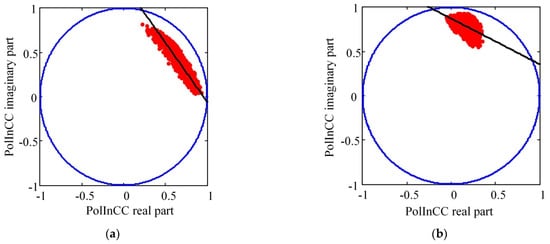
Figure 1.
Distribution of PolInCCs (red dots) and straight line (black) fitting in a single pixel based on (a) L-band and (b) X-band data.
For an X-band wave, its penetration depth in the forest is limited due to its short wavelength. The PolInCCs under different polarization states in a single-resolution unit are not different, and the distribution of the scattered dots which represent PolInCCs is concentrated. At this time, the PolInCCs in most of the pixels may not be directly fitted to obtain the ground phase. In addition, due to the short wavelength, the medium in the forest is no longer an anisotropic homogeneous scattering body, that is, the extinction coefficient in the forest is related to the polarization state of the wave. In this scenario, the effective solution range of the VCC is limited by the extinction coefficient range. That is, the VCC farthest from the ground phase point in the traditional coherence coefficient distribution range is no longer applicable to the estimation of forest height when using X-band data The question of how to find the correct ground phase point and the effective VCC is a difficult problem to be solved in relation to forest height estimation using X-band data.
To cope with the issues described above, a new strategy based on the frequency segmentation (FS) of SAR images from different polarization channels (HH, HV, and VV) is introduced in this paper [40]. The PolInCC range of the original SAR image under different polarizations is expanded by means of the PolInCCs of the sub-view interferometric pair after the FS operation in order to obtain the accurate ground phase. For the judgment of the effective VCC, part of the fitting line determined by the expanded PolInCC range is intercepted by the FECCC, so as to improve the accuracy of the estimation of the forest height. The remainder of this paper is organized as follows. Section 2 describes the details, principles, and procedure of the new proposed strategy. In Section 3, we report on our experiments on X-band airborne PolInSAR data, which were conducted to validate the effectiveness of the proposed method. Comparisons with commonly used and typical forest height estimation algorithms, as well as a discussion, are presented in this section. Finally, the research findings and their implications are discussed in Section 4 and conclusions are drawn in Section 5.
2. Methods
2.1. PolInSAR Data Spectrum Segmentation
Because the penetration of X-band electromagnetic waves in forest is generally weak, the PolInCCs obtained under different polarization states are not very different, and the PolInCC distribution in the complex unit circle is relatively concentrated. Thus, it is impossible to obtain the surface interferometric phase in the forest by straight-line fitting the distribution of the coherence coefficient in most of the resolution units in the forest area with X-band data. In order to expand the distribution range of the PolInCCs in the complex unit circle, in this section we introduce a method of azimuthal spectrum division using different polarization channels. The direction of the fitting line of the PolInCCs is modified based on the PolInCCs of sub-view SAR images after spectrum division, so that the accurate ground phase of the forest can be estimated.
The azimuth resolution of an SAR image is determined by observing the target at different azimuth angles to form a synthetic aperture, and then the signal in the synthetic aperture is formed via the coherent accumulation of pulses. The relative motion between the radar platform and the target forms a changing Doppler frequency and a changing observation angle in the synthetic aperture accumulation time. The range of observation angles determines the Doppler bandwidth and ultimately affects the azimuth resolution . The algebraic relationship between them is
where is the wavelength. The variable is the velocity of the radar platform. For a fixed Doppler frequency, the relationship between and the corresponding observation angle is
The SAR image is transformed by means of a fast Fourier transform (FFT) and the frequency spectrum is segmented along the azimuth direction, which is equivalent to segmenting the image into several sub-view SAR images under different observation angles. Then, the sub images in the frequency domain are transformed to the time domain by means of an inverse fast Fourier transform (IFFT). Compared with the original SAR image, the resolution of the sub-view images is slightly decreased. The sub-view images correspond to different observation angles, the scattering information for the same ground object in different sub-views is different, and the scattering information for sub-view images in different polarization channels is also different. In the forest, the scattering phase center heights of electromagnetic waves are different. The specific process of PolInSAR data segmentation involves performing an FFT on the azimuth direction of the data obtained from different polarization channels (HH, HV, and VV channels) between the two interferometric channels, and the range direction is not operated upon. Then, the azimuth spectrum of each polarization channel is divided into three parts uniformly, and each part is transformed into the time domain. We perform the interferometric process with the sub-view of the corresponding polarization channel based on the azimuth view angle to obtain the sub-view PolInCC map for different polarization channels. The distribution positions of the PolInCCs for different polarization channels of the sub-images in the same resolution unit are also different in the complex unit circle, which is physically manifested as different scattering phase centers of electromagnetic waves in the forest. The resolution of the sub-view is low, which is equivalent to increasing the electromagnetic wave on the basis of the original observation angle, and is furthermore equivalent to increasing the penetration depth of electromagnetic wave in the vegetation. Thus, the distribution of PolInCCs is different from that of the original image. Therefore, the distribution range of the PolInCCs in the original PolInSAR image can be effectively expanded, and the fitting direction of the coherence coefficient can be modified to obtain a more accurate ground phase. The process above is called the FS process of PolInSAR data. The relationship between the spectrum division and the azimuth angle of view is shown in Figure 2.
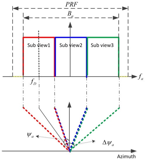
Figure 2.
Schematic diagram of the frequency spectrum of PolInSAR data.
2.2. Polarization Coherent Scattering Model Considering Polarization Characteristics
In a forest, in the two-layer coherent scattering model, the scattering coherence matrix characterizing a forest feature can be described as [41,42]
where and are the pulse function and the rectangular window function. is the reference ground elevation. and are the scattering coherence matrices of the ground and the forest, respectively. Under the assumption that the ground target has reflection symmetry, the two kinds of coherence matrices can be expressed as
where and are the scattering amplitudes of the ground and forest, respectively. Considering the X-band, the electromagnetic wavelength is equivalent to the size of the branches and leaves in the forest, and the extinction coefficient of the electromagnetic wave in the forest is related to the polarization state of the electromagnetic wave. Without considering time decorrelation, the PolInCC is
Since the azimuth sub-aperture has a direct relationship with the azimuth observation angle, we can express the relationship between the azimuth observation angle and the RVoG model by means of an analogy with the incidence angle in the range direction in the RVoG model. Therefore, the expressions of the cross-correlation matrix and the autocorrelation matrix are as follows:
where is the equivalent extinction coefficient related to the polarization characteristics in the forest. The angle is the azimuth observation angle of the sub-aperture center. The PolInCCs obtained via the rearrangement of (6) are expressed as
where . and are the VCC, including the extinction coefficient related to the polarization state and the ground volume amplitude ratio (GVAR), respectively. The expression is
where is the vertical effective wave. Formula (9) represents a polarization-coherent scattering model considering polarization characteristics, in which the extinction coefficient is related to the polarization state of the electromagnetic wave. With the change in the polarization state, the extinction coefficient of the electromagnetic wave also changes. Therefore, the form of the distribution of PolInCCs in the complex unit circle is shown as a certain region [41,42]. Since the added azimuth angle is located at the denominator of the power index, it can be understood from the perspective of the formula that it is equivalent to expanding the range of the VCC and increasing the penetration depth of the electromagnetic wave in the vegetation, which further proves our previous hypothesis.
For each polarization state, when the GVAR gradually increases, changes from 0 to 1. For each individual scattering coherence coefficient point, a line from the ground scattering phase point to the VCC (including the ground phase) point can be drawn. Under different polarization states, the PolInCC distribution forms an approximate triangular region. The size of the triangular region is related to the range of extinction, and its boundary corresponds to the maximum and minimum extinction coefficients, respectively. The PolInCCs at the boundary are generally the coherence coefficients based on their characteristic polarization. In Figure 3, the cyan area depicts the distribution range of PolInCCs related to polarization characteristics.
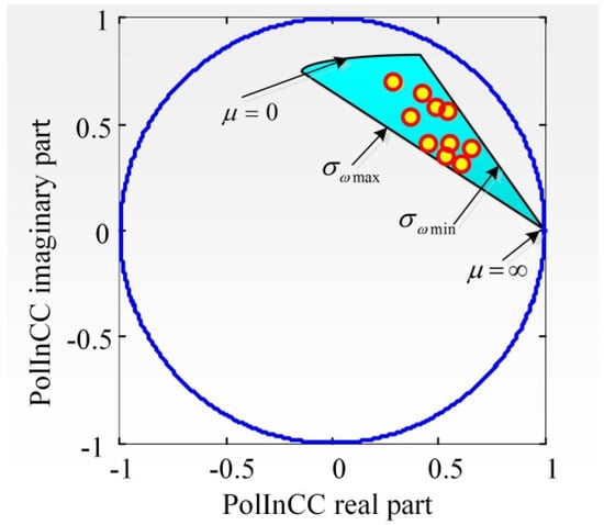
Figure 3.
Distribution area of PolInCCs, considering polarization characteristics.
When the maximum and minimum extinction coefficients in the PolInCCs and the ground phase point in the forest are determined, two curves in the complex unit circle can be obtained on the basis of the relationship between the extinction coefficient and the tree height in the VCC. An approximate quadrilateral coherence coefficient distribution area can be determined by combining the two boundaries of the coherence coefficient distribution area under different polarization states. In this distribution area, the VCC is considered as the effective VCC in the forest under different polarization states. Then the ground phase is removed from the effective VCC. After that, the VCCs in this area are compared with LUT to obtain a set of height values, and the final forest canopy height can be obtained by calculating the average. Figure 4 shows the distribution range of the effective VCC. The pink approximately quadrilateral area in the figure is the distribution area of the effective VCC, related to polarization characteristics.
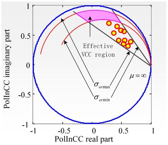
Figure 4.
Schematic diagram of the effective VCC distribution region.
For the ground phase in the estimation of forest height in the X-band, the FS method is used to expand the distribution range of PolInCCs, and then the ground phase is obtained by means of the straight-line fitting method. It can be seen from the expression of the VCC that the determination of the maximum and minimum extinction coefficients requires a known forest height. In the VCC curve with the extinction coefficient as an independent variable, the maximum and minimum extinction coefficients can be found based on the intersection of the boundary line of the PolInCCs and the curve (at this time, the amplitude ratio of the ground to the volume is approximately 0). In practice, the forest height is unknown in the process of estimation. The maximum and minimum values of the extinction coefficient cannot be determined in advance. The research in the literature [43] shows that the extinction coefficient of a forest area above 10 m using X-band data is about 0.4 db/m. Therefore, we restricted the extinction coefficient range to dB/m. The final forest height was calculated in the effective volume scattering region using the extinction coefficient in this range.
2.3. Estimation Process of Forest Height
According to the FS method applied to PolInSAR data and polarization coherent scattering model considering polarization characteristics that was introduced above, the detailed process of forest height estimation using X-band data is given below.
(1) PolInSAR data FS.
First, the azimuth direction of the full polarization data (HH, HV, and VV channels) from the two interferometric channels in the PolInSAR data was transformed to the frequency domain, respectively, and the range direction was not discarded. Then, the frequency domain iwass divided into three consecutive parts. We transformed all these parts into the time domain to obtain 18 sub SAR images with different polarizations, i.e., nine pairs of sub-view interferometric images.
(2) Extending the PolInCCs to solve the ground phase.
Using the nine sub-view interferometric image pairs obtained by means of FS, nine sub view PolInCCs maps could be obtained. For each pixel unit of the original images, the interferometric coherence matrix of the original image was used to obtain a number of PolInCC distribution points in the random scattering state. In Figure 5, the distribution diagram of the coherence coefficient in a pixel unit is shown. The coherence coefficient points in the figure depicted in yellow are the PolInCC points in several random states in the original image, and the points depicted in purple are the PolInCC points in the sub-view interferometric images under different polarization states. Line fitting based on the least squares method was performed by combining the PolInCC points of the nine sub-views obtained in the specific pixel point. The fitting line and the unit circle intersected at two points. Assuming that the forest height is lower than , and are the phase values corresponding to the two intersections of the line and the unit circle. For traditional forest height estimation, the topographic phase point is selected according to the nearest intersection points to the PolInCC point of HH + VV polarization channel (the yellow coherence coefficient point in Figure 5). This may be effective for L-band tree height inversion. However, for X-band height inversion, this approach will lead to a large error. In the X-band, the coherence coefficient is relatively concentrated in the unit circle, the intersection point with a distance close to the coherence coefficient of the HH + VV channel is not necessarily a terrain phase point, and the probability of it being an invalid point is very high, so there will be a large error in the terrain measurement obtained. It can be seen from the interference principle that when the vertical effective wave is greater than zero, the phase change of the electromagnetic wave in the vegetation from the treetop to the tree bottom is reflected in the unit circle as a counterclockwise change [44,45]. On the contrary, when the vertical effective beam is less than zero, the phase change of the electromagnetic wave in the vegetation from the treetop to the tree bottom is reflected in the unit circle as a clockwise change. Therefore, when the sign of is determined, we can easily determine the terrain phase of the two intersection points according to the direction of phase change and the error in the terrain phase estimation can be reduced greatly. It is noteworthy that here we assume that the phase change of the electromagnetic wave in the vegetation does not exceed half a phase period, that is, it does not exceed . In this paper, the topographic phase can be judged according to the following criteria:
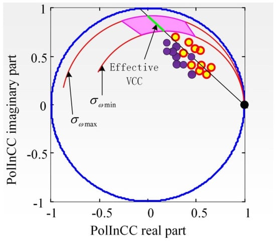
Figure 5.
Schematic diagram of forest canopy height estimation process using X-band data.
That is, we judged the ground phase based on the difference between and and the vertical effective wave . Through the expansion of the distribution range of the PolInCCs and the ground phase judgment criterion, the probability of an erroneous judgment of the ground phase point and the estimation error of the ground phase can be effectively reduced.
(3) Determining the effective solution range of the VCC.
In principle, for a forest volume with an extinction coefficient related to the polarization state, the effective solution of the VCC is determined based on the approximate quadrilateral surrounded by the boundary of the PolInCC distribution area and the two curves, with a given extinction coefficient range. In practice, if the PolInCC distribution is not uniform, the opening angle corresponding to the boundary will be too large, and the range of the quadrilateral enclosed by it will be too large. This situation results in the range of the effective VCC being too large, making it impossible to determine the accurate VCC. To address this issues, the line segment on the fitting line intercepted by the two coherence coefficient curves under the specific extinction coefficient range (such as dB/M) is used as the effective solution region of the VCC. The green line segment shown in Figure 5 indicates the selected effective VCC distribution area.
(4) Obtaining the forest height.
In the effective solution area of the obtained volume coherence coefficient, several coherence coefficient points were discretely selected to compensate for the ground phase estimated previously, and then several forest height values were found according to comparisons with LUT. Finally, the forest height of this pixel was obtained by averaging these height values found by means of LUT.
3. Results
To verify the effectiveness of the proposed method for forest height estimation using the X-band data, which combines the FS results of PolInSAR data, the ground phase judgement, and the VCC model considering polarization characteristics, in this paper, verification was carried out using airborne-measured X-band data. For this purpose we implemented the Chinese airborne N-SAR system in the Yellow River beach area in the east of Shaanxi province, China. The test data consisted of the full set of polarimetric interferometry data. The ground in this area is relatively flat and the forest in this area is large, with artificially planted trees, and dense. The average height of the trees, measured via random sampling (45 samples), in the forest was 19.29 m. Figure 6a depicts an optical map of this area from Google Earth, and Figure 6b presents a Pauli base polarization decomposition map of the full-polarization SAR data. The data size was 8192 × 4096 pixels.
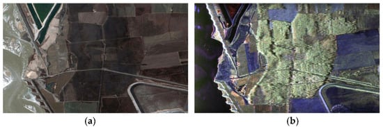
Figure 6.
Airborne PolInSAR experimental data. (a) Google Earth optical map of forest area. (b) Pauli base PolSAR decomposition map.
Figure 7a–c depict amplitude maps of PolInCCs for different sub-views of the HV polarization channel after FS processing. The number of sub-views is consistent with the number of sub-views shown in Figure 2 and the corresponding viewing angles. It can be seen that the PolInCCs of the forest area under different sub-views exhibited obvious changes. The amplitude of the PolInCCs of sub view 1 was slightly lower than those of the other sub-views. One possibility is that the polarization scattering characteristics of the ground objects from the perspective of the two interferometric channels were greatly different when the viewing angle was larger, thus resulting in a decrease in the coherence of the two channels. Figure 7d depicts a statistical curve of the PolInCCs’ amplitudes in different sub-views of the HV polarization channel in the above-described forest area. It can be seen that the coherence coefficient of sub-view 1 was significantly lower than those of the other two sub-views, and the coherence coefficients of sub-view 2 and sub-view 3 were close to each other, but overall the coherence coefficient of sub-view 2 was slightly higher. This indicates that the scattering information for the same ground object in different sub-views of the HV polarization channel was different, so it can be inferred that the scattering information for the sub-views of different polarization channels were also different, and the scattering phase center height of the electromagnetic wave was different in the forest. Thus, the polarization scattering information in the forest could be further expanded, so as to accurately retrieve the parameters in the forest.
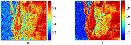
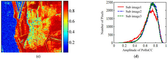
Figure 7.
Amplitudes of PolInCCs for different sub-views of the HV channel. (a) amplitude of PolInCCs for sub-view 1, (b) amplitude of PolInCCs for sub-view 2, (c) amplitude of PolInCCs for sub-view 3, and (d) statistical curve of PolInCCs’ amplitudes in different sub-images.
To examine the relationship between the forest and the scattering phase, the interferometric phase images of different sub-views of HV channel images were obtained from the complex PolInCCs. Before this operation, one of the most significant steps was to calibrate the attitude error, mainly caused by the roll angle, in terms of the inertial navigation system (INS). Without this procedure, the interferometric phase fringe would be severely bent, although the ground in the forest area is flat, thus resulting in great errors in the final forest height estimation. After the attitude calibration, the interferometric phase fringe of the sub-views images was nearly straight along the azimuth in the images in terms of the flat ground context. Figure 8 shows the phase fringes of different sub-views of the HV channel, and the phase results of different sub-views obtained after removing the flatting effect. Based on the phase fringe maps, we can see that, on the left side of the map, the phase was almost noise. Because the scene on the left side was the yellow river, the decorrelation effect was very remarkable in the torrents.
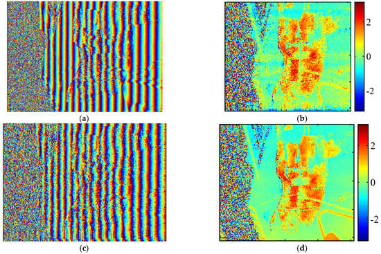
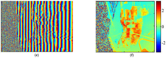
Figure 8.
Phases of different sub-views of the HV channel. (a,c,e) are the interferometric phases of sub-image 1, sub-image 2, and sub-image 3, respectively. (b,d,f) are the remaining phases of sub-image 1, sub-image 2, and sub-image 3, respectively, after removing the flatting effect.
It can be seen in Figure 8 that the straight phase fringes were smeared in the forest areas. This proves that the scattering phase center heights of waves under different polarizations were different in the forest. After removing the flatting effect, the phase of the forest area was significantly higher than that of the bare surface area, the phase of the surface area was close to zero degrees, and the phase of the vegetation area was close to two degrees. On the other hand, due to the weak penetration depth of X-band waves, the phase differences of the PolInCCs of the sub-views were not obvious. As they were similar to the segmentation process for the HV channel, we will not repeat the FS results applied to the other polarization channels. We describe the process of tree height inversion in a single pixel of the measured data in detail below, as shown in Figure 9.
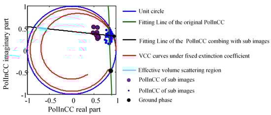
Figure 9.
Estimation process of forest height in a pixel unit using real X-band PolInSAR data.
Figure 9 shows the middle-process part of the estimation results obtained using the forest height estimation method proposed in this paper in a pixel resolution unit of the forest area. The blue points in the figure indicate the distribution range of the PolInCCs of the original image under different polarization states. It can be seen that the distribution of the PolInCCs of this pixel point was relatively concentrated. Conventionally, the ground phase (black points in the figure) can be determined via straight-line fitting with these dots (blue points in the figure). The figure shows that the ground phase (after removing the flat effect) obtained via straight-line fitting (green straight line), estimated using only the PolInCC points of the original image, displayed a large error (−20.7°) compared with the actual ground phase (nearly 0°). However, the ground phase error obtained based on the expanded distribution range of the PolInCCs was small. By using the PolInCCs from the sub-view interferogram obtained by means of FS (purple points in the figure) and the original PolInCCs jointly, the straight-line fitting (black straight line) approach resulted in a good estimation of the ground phase (15.2°), which was closed to 0°, compared with the traditional method. In the experiment, we also used the aforementioned judgment criteria to further ensure the accuracy of the ground phase. The extinction coefficient was set to vary from 0.2 db/m to 0.6 db/m. The change curve of the PolInCCs of the corresponding volume at the boundary point is represented by the red curve in Figure 9. The line segment (cyan line segment) in the straight fitting line (black line) intercepted by the two curves indicates the distribution range of the effective VCC (including the ground phase). It can be seen that this was far from the real PolInCC distribution. In the traditional estimation of forest height, due to the ambiguity of the distribution of the VCC, only the coherence coefficient of the HV polarization channel or the point farthest from the ground phase point in the distribution range of PolInCCs can be used indirectly as the effective VCC. However, in the X-band, the VCC still exhibits a large amount of ambiguity when using the method above, resulting in a serious underestimation of the estimation results. The new method can effectively reduce the ambiguity of the VCC by ensuring an accurate estimation of the ground phase. Finally, the accurate estimation of forest canopy height using X-band data was achieved.
The method proposed in this paper includes three key steps. The first involves using FS to expand the distribution range of the PolInCCs. After the straight-line fitting process is completed, the ground phase is inverted using the judgment criterion. Then, the distribution range of the effective VCC is selected. In order to verify the effectiveness of the proposed method, we therefore introduced four common height estimation methods to compare them with the new estimation strategy. These methods represent a combination of the retention of one of the three steps and the substitution of conventional methods. The first method does not use the PolInCCs of the sub-view to expand the phase distribution, and the ground phase is inverted using the distance between the intersection of the traditional fitting line with the circle and the HH + VV PolInCC dot. The VCC is obtained via the phase diversity (PD) method. We abbreviate this method as NePhVpd. The second method does not use the PolInCCs of the sub-view to expand the phase distribution, but the ground phase is judged using the criteria introduced in this paper, and then the VCC is also obtained via PD. We abbreviate this method as NePcVpd. The third method does not use the PolInCCs of the sub-view to expand the phase distribution, but the ground phase is judged using our criteria, and the distribution area of the effective VCC is constrained by a given range, as mentioned above, and we abbreviate this method as NePcVe. The fourth method involves using the PolInCCs of the sub-view to expand the phase distribution, and the ground phase is also judged using the criteria presented here, but the distribution area of the effective VCC is obtained via PD. We abbreviate this method as EPcVpd. The final method is the estimation strategy proposed in this paper. We abbreviate it as EPcVe. In this method, the phase distribution is first expanded using the coherence coefficient of the sub-view, and the ground phase is judged using the criteria introduced in this paper. Then, the distribution area of the VCC is constrained by means of a given range. All the forest height estimation results are carried out by matching the selected VCC with the LUT. To describe the methods intuitively, we show them in Table 1.

Table 1.
Different forest height estimation methods for X-band data.
Figure 10 shows part of the height estimation results obtained using the different methods described above. The two-dimensional results were partial results selected from areas with uniform tree distributions in SAR images. Without an auxiliary LiDar, for the sake of obtaining the true values of the forest, we measured the trees manually with a height indicator (the accuracy was 0.1 m) in this area by conducting random sampling (45 samples) in the forest, and the average height was found to be 19.29 m. Since the height estimation of only one pixel in the images is considerably time-consuming, obtaining the tree height results for the whole image using all the methods selected for comparison would represent a huge workload. In order to illustrate the effectiveness of our method concisely and intuitively, we only took part of the tree height images for inversion, and the cross-section was used for comparison. The selected data size was 11 × 140 pixels. We constrained the tree height range of the estimation results from 0 m to 40 m. According to the two-dimensional results shown in Figure 10, a large amount of tree heights were underestimated or overestimated by the NEPhVpd method. This indicates that the conventional estimation method was no longer applicable when using X-band data. Neither the ground phase nor the VCC had considerable errors. For the NEPcVpd method, most of the tree heights were underestimated. One possible reason for this is that the VCC determined by means of PD is different from the effective VCC. For the NEPcVe method, some of the estimation results were overestimated compared with the NEPcVpd method. This indicates that the ground phase error was the major reason leading to the misinterpretation, though the phase was selected based on the judgment criteria and the VCC was constrained. For the EPcVpd method, we can see that most of the estimation results were around 20 m, which was very close to the true value. Compared with the NEPcVpd method, this reveals that the expansion of the PolInCCs is essential for height estimation using X-band data. However, due to the lack of a VCC constraint, there was still a certain amount of overestimation. For the EPcVe method, i.e., our new strategy for X-band forest height estimation, most of results were around the true value, and the results were very robust except for a few errors at the data edge. In other words, the three steps in our method are indispensable. Moreover, profiles along the range of the forest area were included in the experimental results. It can be seen that the distribution of the forest heights estimated using our method was within the range of 19 m to 24 m, and the estimation result was relatively stable, whereas the heights estimated using other methods were distributed within the range of 0 m to 40 m, indicating that these estimation results had a large error.
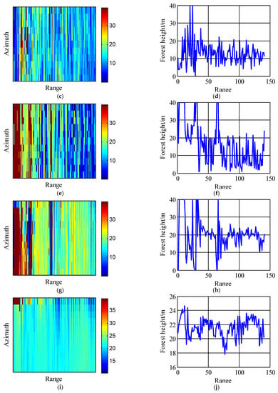
Figure 10.
Forest height estimation results using measured X-band data, obtained using different methods. (a,b) are the results of NEPhVpd, (c,d) are the results of NEPcVpd, (e,f) are the results of NEPcVe, (g,h) are the results of EPcVpd, and (i,j) are the results of EPcVe, respectively. (a,c,e,g,i) are the two-dimensional height estimation results and (b,d,f,h,j) are the profiles of height along the range in the same azimuth bins.
Furthermore, we calculate the means and RMSE values of the tree height estimates obtained using different methods, and the results are shown in Table 2. It can be seen from the table that the average tree heights estimated using the different methods exhibited error values of 29.65%, 30.84%, 15.71%, 12.60%, and 12.80%, respectively. The estimation errors of the proposed method and the EPcVpd method were close to 10%, whereas the RMSE of the estimation result of the proposed method was much smaller than that of the other methods. Finally, we obtained the forest height estimation results for the whole image using our method, as shown in Figure 11.
Table 2.
Mean and RMSE values of forest height estimation results obtained using different methods based on X-band data.
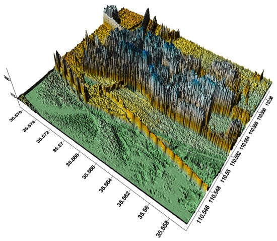
Figure 11.
Three-dimensional forest height estimation result of the whole image.
4. Discussion
In this paper, the estimation of forest canopy height using PolInSAR data from the X-band was studied. First, for the X-band, because the penetration depth of electromagnetic waves in forests is relatively shallow, we introduced the azimuth FS operation for SAR images with different polarization channels. As a first step in this field of exploration, we implemented this operation only on the HH, HV, and VV channels, and the segmentation was carried out in only three parts. As a reasonable deduction, the expansion of the PolInCCs could be more accurate and robust if we divided the frequency domain into more parts or if we introduced more polarization channels, e.g., HH + VV and HH-VV channels. Certainly, this would require a compromise between the complexity of the algorithm (that is, the time-consumption) and the accuracy of the algorithm. A detailed analysis of influence of FS numbers and polarization channels on the estimation accuracy should be undertaken in future studies. Moreover, the range of the extinction coefficient for the constraint of the effective VCC was determined based on an empirical value. This inevitably expanded the VCC estimation error. Investigating how to determine the exact range of this value according the boundary of the PolInCCs is an essentialtask for future studies.
For an assessment of the final estimation results, one reasonable verification method would be to acquire the true value of each pixel by means of LiDar measurements corresponding to the PolInSAR images, and each pixel should be compared to test the method’s feasibility. Unfortunately, no such devices were available under our research conditions. Furthermore, the capabilities of the new approach need to be studied further in regard to whether the strategy is suitable for more other X-band airborne data, as well as for other vegetation types, such as boreal coniferous forests. Furthermore, it is of great significance to study whether the strategy is equally effective for space-borne PolInSAR data, as this is significant in regard to large-scale forest estimation.
We investihated the forest height using the airborne X-band PolInSAR data with the assumption of flat terrain, not taking the terrain into account. Due to the presence of shadows, overlays and top-to-bottom overlaps may occur with large terrain fluctuations, thus leading to a severe degradation of estimation accuracy. In future studies, areas with sloped terrain should be considered. The S-RVoG model can be applied to this new strategy, which is what we intend to do in the near future.
5. Conclusions
To solve the issues desribed above, a new strategy based on the FS of SAR images from different polarization channels (HH, HV, and VV) has been proposed in this paper. Several sub-view interferometric images for different polarizations were obtained by means of spectral segmentation. The range of PolInCCs of the original SAR image under different polarization levels was expanded using the PolInCCs of the sub-view interferometric pair. Then, the extended PolInCCs were fitted using the least squares method, and the accurate ground phase was obtained based on the ground phase judgment criteria. For the judgment of the effective VCC, after constraining the extinction coefficient range, the part of the fitting line of the expanded PolInCC range that was intercepted by the fixed extinction coefficient curve was averaged, so as to improve the accuracy of the estimation of forest height. The final forest height was retrieved from the average value of tree height within the constraint range of the extinction coefficient on the fitting line. The proposed method was validated using X-band airborne data, and the results showed that the proposed method could effectively retrieve the forest canopy height using X-band data.
Author Contributions
J.X. was the principal author of this manuscript, was responsible for its conception, wrote the majority of the manuscript, and contributed to all phases of the investigation. Y.Z. and L.L. contributed to the interpretation of the methods and provided suggestions regarding the structure. L.Z. and L.L. contributed to the data processing. All authors have read and agreed to the published version of the manuscript.
Funding
This research received no external funding.
Acknowledgments
The authors express their sincere gratitude to the anonymous reviewers and editor, whose contribution was critical for improving the quality of this manuscript.
Conflicts of Interest
The authors declare no conflict of interest.
References
- Wiley, C.A. Synthetic aperture radars. IEEE Trans. Aerosp. Electron. Syst. 2007, AES–21, 440–443. [Google Scholar] [CrossRef]
- Pang, Y.; Zhao, F.; Zeng-Yuan, L.; Zhou, S.F.; Deng, G.; Liu, Q.W.; Chen, E.X. Forest height inversion using airborne Lidar technology. J. Remote Sens. 2008, 12, 158. [Google Scholar]
- Lee, S.K.; Kugler, F.; Papathanassiou, K. Multibaseline polarimetric SAR interferometry forest height inversion approaches. In Proceedings of the ESA PolInSAR Workshop, Frascati, Italy, 24–28 January 2011; pp. 24–28. [Google Scholar]
- Wang, C.C.; Wang, L.; Fu, H.Q.; Xie, Q.H.; Zhu, J.J. The Impact of Forest Density on Forest Height Inversion Modeling from Polarimetric InSAR Data. Remote Sens. 2016, 8, 291. [Google Scholar] [CrossRef]
- Zhen, L.I.; Guo, M.; Wang, Z.Q.; Zhao, L.F. Forest-height inversion using repeat-pass spaceborne PolInSAR data. Sci. China Earth Sci. 2014, 57, 1314–1324. [Google Scholar]
- Lee, J.S.; Pottier, E. Polarimetric radar imaging: From basics to applications. Int. J. Remote Sens. 2002, 33, 333–334. [Google Scholar]
- Lee, J.S.; Grunes, M.R.; Ainsworth, T.L.; Du, L.J.; Schuler, D.L.; Cloude, S.R. Unsupervised classification using Polarimetric decomposition and the complex Wishart classifier. IEEE Trans. Geosci. Remote Sens. 1999, 37, 2249–2258. [Google Scholar]
- Lee, J.S.; Grunes, M.R.; Grandi, G.D. Polarimetric SAR speckle filtering and its implication for classification. IEEE Trans. Geosci. Remote Sens. 1999, 37, 2363–2373. [Google Scholar]
- Cloude, S.R.; Corr, D.G.; Williams, M.L. Target detection beneath foliage using polarimetric synthetic aperture radar interferometry. Waves Random Media 2004, 14, S393–S414. [Google Scholar] [CrossRef]
- Sletten, M.; Brozena, J. Detection of targets beneath foliage using aspect-angle variation of the polarimetric SAR response. In Proceedings of the IEEE Radar Conference, Cincinnati, OH, USA, 19–23 May 2014; pp. 0296–0297. [Google Scholar]
- Bamler, R. Synthetic aperture radar interferometry. Inverse Probl. 1998, 14, 12–13. [Google Scholar] [CrossRef]
- Rosen, P.A.; Hensley, S.; Joughin, I.R.; Li, F.K.; Madsen, S.N.; Rodriguez, E.; Goldstein, R.M. Synthetic aperture radar interferometry. IEEE Proc. 2002, 88, 333–382. [Google Scholar] [CrossRef]
- Rodriguez, E.; Martin, J.M. Theory and design of interferometric synthetic aperture radars. IEE Proc. F 1992, 139, 147–159. [Google Scholar] [CrossRef]
- Cloude, S.R.; Papathanassiou, K.P. Polarimetric SAR interferometry. Remote Sens. Technol. Appl. 1999, 36, 1551–1565. [Google Scholar] [CrossRef]
- Cloude, S.R.; Papathanassiou, K.P. Three-stage inversion process for polarimetric SAR interferometry. IEE Proc. Radar Sonar Navig. 2003, 150, 125–134. [Google Scholar] [CrossRef]
- Li, Z.; Guo, M. A new three-stage inversion procedure of forest height with the improved temporal decorrelation RVoG model. In Proceedings of the IEEE International Geoscience and Remote Sensing Symposium, Munich, Germany, 22–27 July 2012; pp. 5141–5144. [Google Scholar]
- Qi, Z.; Tiandong, L.; Zegang, D.; Tao, Z.; Teng, L. A modified three-stage inversion algorithm based on R-RVoG model for Pol-InSAR data. Remote Sens. 2016, 8, 861. [Google Scholar]
- Garestier, F.; Dubois-Fernandez, P.C.; Papathanassiou, K.P. Pine forest height inversion using single-pass X-Band PolInSAR data. IEEE Trans. Geosci. Remote Sens. 2008, 46, 59–68. [Google Scholar] [CrossRef]
- Praks, J.; Kugler, F.; Papathanassiou, K.P.; Hajnsek, I.; Hallikainen, M. Height estimation of boreal forest: Interferometric model-based inversion at L- and X-Band versus HUTSCAT profiling scatterometer. IEEE Geosci. Remote Sens. Lett. 2007, 4, 466–470. [Google Scholar] [CrossRef]
- Praks, J.; Kugler, F.; Papathanassiou, K.; Hallikainen, M. Forest height estimates for boreal forest using L and X band Pol-InSAR and HUTSCAT scatterometer. Proc. Int. Workshop Appl. Polarim. Polarim. Interferom. 2014, 644, 8. [Google Scholar]
- Sadeghi, Y.; St-Onge, B.; Leblon, B.; Simard, M.; Papathanassiou, K. Mapping forest canopy height using TanDEM-X DSM and airborne LiDAR DTM. In Proceedings of the IEEE Geoscience and Remote Sensing Symposium, Quebec City, QC, Canada, 13–18 July 2014; pp. 76–79. [Google Scholar]
- Sohrabi, H. Estimating mixed broadleaves forest stand volume using DSM extracted from digital aerial images. ISPRS—International Archives of the Photogrammetry. Remote Sens. Spat. Inf. Sci. 2012, XXXIX–B8, 437–440. [Google Scholar]
- Mercer, B.; Zhang, Q.; Schwaebisch, M.; Denbina, M. Extraction of DTM beneath forest canopy using a combination of X-band InSAR and L-band PolInSAR data. In Proceedings of the European Conference on Synthetic Aperture Radar, VDE, Aachen, Germany, 4–10 June 2010; pp. 1–4. [Google Scholar]
- Sadeghi, Y.; St-Onge, B.; Leblon, B.; Simard, M. Canopy Height Model (CHM) derived from a TanDEM-X InSAR DSM and an airborne Lidar DTM in boreal forest. IEEE J. Sel. Top. Appl. Earth Obs. Remote Sens. 2016, 9, 381–397. [Google Scholar] [CrossRef]
- Zhang, L.; Zou, B.; Zhang, J.; Zhang, Y. Inversion of Forest Parameters Based on Genetic Algorithm using L-Band Polinsar Data. In Proceedings of the 2006 International Conference on Image Processing, Atlanta, GA, USA, 8–11 October 2006; pp. 2325–2328. [Google Scholar]
- Mercer, B.; Zhang, Q.; Schwaebisch, M.; Denbina, M. 3D topography and forest recovery from an L-BAND single-pass airborne PolInSAR system. In Proceedings of the 2009 IEEE International Geoscience and Remote Sensing Symposium, Cape Town, South Africa, 12–17 July 2009; pp. III-33–III-36. [Google Scholar]
- Garestier, F.; Dubois-Fernandez, P.C.; Champion, I. Forest height inversion using high-resolution p-band Pol-InSAR data. IEEE Trans. Geosci. Remote Sens. 2008, 46, 3544–3559. [Google Scholar] [CrossRef]
- Oleg, A.; Yrj, R.; Tuomas, H.; Jaan, P. Polarimetric alos palsar time series in mapping biomass of boreal forests. Remote Sens. 2017, 9, 999. [Google Scholar]
- Ghasemi, N.; Tolpekin, V.; Stein, A. Assessment of forest above-ground biomass estimation from polinsar in the presence of temporal decorrelation. Remote Sens. 2018, 10, 815. [Google Scholar] [CrossRef]
- Managhebi, T.; Maghsoudi, Y.; Valadan-Zoej, M.J. Four-stage inversion algorithm for forest height estimation using repeat pass polarimetric sar interferometry data. Remote Sens. 2018, 10, 1174. [Google Scholar] [CrossRef]
- Xing, C.; Zhang, T.; Wang, H.; Zeng, L.; Yang, J. A novel four-stage method for vegetation height estimation with repeat-pass polinsar data via temporal decorrelation adaptive estimation and distance transformation. Remote Sens. 2021, 13, 213. [Google Scholar] [CrossRef]
- Sun, X.; Wang, B.; Xiang, M.; Zhou, L.; Jiang, S. Forest height estimation based on p-band pol-insar modeling and multi-baseline inversion. Remote Sens. 2020, 12, 1319. [Google Scholar] [CrossRef]
- Sun, X.; Wang, B.; Xiang, M.; Jiang, S.; Fu, X. Forest height estimation based on constrained gaussian vertical backscatter model using multi-baseline p-band pol-insar data. Remote Sens. 2019, 11, 42. [Google Scholar] [CrossRef]
- Sun, X.; Wang, B.; Xiang, M.; Fu, X.; Li, Y. S-rvog model inversion based on time-frequency optimization for p-band polarimetric sar interferometry. Remote Sens. 2019, 11, 1033. [Google Scholar] [CrossRef]
- Chen, W.; Zheng, Q.; Xiang, H.; Chen, X.; Sakai, T. Forest Canopy Height Estimation Using Polarimetric Interferometric Synthetic Aperture Radar (PolInSAR) Technology Based on Full-Polarized ALOS/PALSAR Data. Remote Sens. 2021, 13, 174. [Google Scholar] [CrossRef]
- Schlund, M.; Davidson, M.W.J. Aboveground forest biomass estimation combining L- and P-band SAR acquisitions. Remote Sens. 2018, 10, 1151. [Google Scholar] [CrossRef]
- Zhao, L.; Chen, E.; Li, Z.; Fan, Y.; Xu, K. The improved three-step semi-empirical radiometric terrain correction approach for supervised classification of Polsar data. Remote Sens. 2022, 14, 595. [Google Scholar] [CrossRef]
- Zhang, J.; Zhang, Y.; Fan, W.; He, L.; Yu, Y.; Mao, X. A modified two-steps three-stage inversion algorithm for forest height inversion using single-baseline l-band Polinsar data. Remote Sens. 2022, 14, 1986. [Google Scholar] [CrossRef]
- Qi, F.; Liangjiang, Z.; Erxue, C.; Xingdong, L.; Lei, Z.; Yu, Z. The performance of airborne c-band polinsar data on forest growth stage types classification. Remote Sens. 2017, 9, 955. [Google Scholar]
- Haiqiang, F.; Jianjun, Z.; Changcheng, W.; Huiqiang, W.; Rong, Z. Underlying topography estimation over forest areas using high-resolution P-band single-baseline PolInSAR data. Remote Sens. 2017, 9, 363. [Google Scholar]
- Lopez-Sanchez, J.M.; Ballester-Berman, J.D.; Marquez-Moreno, Y. Model limitations and parameter-estimation methods for agricultural applications of polarimetric SAR interferometry. IEEE Trans. Geosci. Remote Sens. 2007, 45, 3481–3493. [Google Scholar] [CrossRef]
- Ballester-Berman, J.D.; Lopez-Sanchez, J.M.; Fortuny-Guasch, J. Retrieval of biophysical parameters of agricultural crops using polarimetric SAR interferometry. IEEE Trans. Geosci. Remote Sens. 2005, 43, 683–694. [Google Scholar] [CrossRef]
- Praks, J.; Antropov, O.; Hallikainen, M.T. Lidar-aided SAR Interferometry studies in boreal forest: Scattering phase center and extinction coefficient at X- and L-band. IEEE Trans. Geosci. Remote Sens. 2012, 50, 3831–3843. [Google Scholar] [CrossRef]
- Xu, G.; Gao, Y.D.; Li, J.W.; Xing, M.D. InSAR Phase Denoising: A Review of Current Technologies and Future Directions. IEEE Geosci. Remote Sens. Mag. 2020, 8, 64–82. [Google Scholar] [CrossRef]
- Gang, X.; Mengdao, X.; Xiang-Gen, X.; Lei, Z.; Yanyang, L.; Zheng, B. Sparse Regularization of Interferometric Phase and Magnitude for InSAR Image Formation Based on Bayesian Representation. IEEE Trans. Geosci. Remote Sens. 2015, 53, 2123–2136. [Google Scholar]


Publisher’s Note: MDPI stays neutral with regard to jurisdictional claims in published maps and institutional affiliations. |
© 2022 by the authors. Licensee MDPI, Basel, Switzerland. This article is an open access article distributed under the terms and conditions of the Creative Commons Attribution (CC BY) license (https://creativecommons.org/licenses/by/4.0/).