Article

A Novel Freeze-Thaw State Detection Algorithm Based on L-Band Passive Microwave Remote Sensing

1
Department of Atmospheric and Oceanic Sciences, Institute of Atmospheric Sciences, Fudan University, Shanghai 200438, China
2
Zhuhai Fudan Innovation Research Institute, Zhuhai 519000, China
3
Institute for Geosciences-Meteorology, University of Bonn, Auf dem Huegel 20, 53121 Bonn, Germany
4
The Plateau Atmosphere and Environment Key Laboratory of Sichuan Province, Chengdu University of Information Technology, Chengdu 610225, China
5
Cloud and Precipitation Exploration Laboratory (CPEX-Lab) of Geoverbund ABC/J, Auf dem Huegel 20, 53121 Bonn, Germany
6
Department of Water Resources, Faculty of Geo-Information Science and Earth Observation (ITC), University of Twente, 7500AE Enschede, The Netherlands
*
Author to whom correspondence should be addressed.
Remote Sens. 2022, 14(19), 4747; https://doi.org/10.3390/rs14194747
Submission received: 27 July 2022 / Revised: 15 September 2022 / Accepted: 17 September 2022 / Published: 22 September 2022
(This article belongs to the Special Issue Microwave Remote Sensing of Soil Moisture)

Abstract

:
Knowing the freeze-thaw (FT) state of the land surface is essential for many aspects of weather forecasting, climate, hydrology, and agriculture. Microwave L-band emission contains rather direct information about the FT-state because of its impact on the soil dielectric constant, which determines microwave emissivity and the optical depth profile. However, current L-band-based FT algorithms need reference values to distinguish between frozen and thawed soil, which are often not well known. We present a new FT-state-detection algorithm based on the daily variation of the H-polarized brightness temperature of the SMAP L3c FT global product for the northern hemisphere, which is available from 2015 to 2021. Exploiting the daily variation signal allows for a more reliable state detection, particularly during the transition periods, when the near-surface soil layer may freeze and thaw on sub-daily time scales. The new algorithm requires no reference values; its results agree with the SMAP FT state product by up to 98% in summer and up to 75% in winter. Compared to the FT state inferred indirectly from the 2-m air temperature and collocated soil temperature at 0–7 cm of the ERA5-land reanalysis, the new FT algorithm has a similar performance to the SMAP FT product. The most significant differences occur over the midlatitudes, including the Tibetan plateau and its downstream area. Here, daytime surface heating may lead to daily FT transitions, which are not considered by the SMAP FT state product but are correctly identified by the new algorithm. The new FT algorithm suggests a 15 days earlier start of the frozen-soil period than the ERA5-land’s estimate. This study is expected to extend the L-band microwave remote sensing data for improved FT detection.

1. Introduction

Spatial patterns and the timing of freeze–thaw (FT) state transitions over land are highly variable; they strongly impact land–atmosphere interactions and thus the weather; the climate; and hydrological, ecological, and biogeochemical processes [1,2,3,4]. In particular, FT state transition leads to differences in hydrological and thermal conductivities/diffusivities, the albedo for shortwave and emissivity for longwave radiation, and latent/sensible heat fluxes [5,6,7]. The albedo is, e.g., higher for frozen than for unfrozen soil, and the water and energy exchange between the land surface and the atmosphere is reduced because of weaker radiation heating and evaporation while frozen. Changes in the FT state dynamics can also signal climate change [8,9] and invoke permafrost carbon feedback [10]. Moreover, ecosystem responses to seasonal FT-state changes are rapid via significant changes in evapotranspiration, soil respiration, plant photosynthetic activity, liquid water availability, vegetation net primary production, and net ecosystem CO2 exchange (NEE) with the atmosphere [11,12,13,14,15]. Thus, the knowledge of the FT state is required for modeling work in the above subjects, which invoke different parametrizations for frozen and unfrozen soil [16,17,18,19,20]. However, FT state estimations from in situ temperature observations are limited in scale, and it is not straightforward to deduce the state from soil, skin, or near-surface air temperature.
In contrast, more direct state information results from the very different microwave dielectric constant for frozen and unfrozen soil [21,22,23]. Accordingly, microwave brightness temperatures (TBs) change sharply during FT state transitions. For instance, NASA’s MEaSUREs (Making Earth System Data Records for Use in Research Environments) program provides two global daily products for the land FT state based on a single-channel algorithm [24]. One covers the years 1979 to 2017 and exploits the 37 GHz channels of three satellite-based passive microwave sensors by exploring the TB values under respective landscape frozen and thawed reference states [25]: the scanning multichannel microwave radiometer (SMMR), the special sensor microwave/imager (SSM/I), and the special sensor microwave imager/sounder (SSMIS). For MEaSUREs, 37 GHz is selected because of its high correlation with the near-surface air temperature. Moreover, lower-frequency L-band sensors on SMOS (Soil Moisture and Sea Salinity) and SMAP (Soil Moisture Active and Passive) are more suitable for FT-change detection because of their deeper penetration depth and their sensitivity to soil moisture [26,27]. For the L band, the difference leads to emissivities of ~0.6 for unfrozen and ~0.9 for frozen soil, with a much deeper penetration depth for the latter [28,29,30]. The cross-polarized gradient ratio (XPGR) at the L band between H and V polarization is used to analyze the SMAP observations. Similar to the higher-frequency single-channel algorithms, the use of XPGR needs reference values for thawed and frozen-soil states and a threshold value for discrimination between both [23,31]. The baseline F/T detection algorithm of SMAP [32] requires at least 20 days to find reference values for the frozen state, which can be challenging for short interim frozen periods induced, e.g., by synoptic-scale cold waves.
Since the XPGR method or the baseline, the F/T detection algorithm of SMAP first needs to identify the frozen/thawed TB reference values, and these results rely on how to construct the reference. Instead, we propose a new FT algorithm that builds its parameters on the TB signal characters. The new FT algorithm has a similar basis to the durinal amplitude variation (DAV) approach [33] applied to higher frequency passive microwave measurements for snow and ice sheet applications [34,35]. It has been proved that the DAV of passive microwave signals are sensitive to FT state changes [33], which are dynamic and complex and vary continuously in space and time. Estimating the FT state changes from the DAV signal is functional because the conditions driving FT changes, e.g., radiation balance and air temperature, change on broad time scales, spanning sub-daily, daily, synoptic, seasonal, and annually interdecadal [36]. Especially in cold arid regions, which are prone to experience FT state transitions, soil moisture fluctuations due to evaporation and precipitation, and their L-band signals, are comparatively low on daily and synoptic scales.
In this study, we use the daily TB cycle and its connection with changing penetration depths during FT state changes to develop a new FT state-detection algorithm, which exploits variance-based filtering on DAV signals ( | Δ T B | ) at the L band between 6 a.m. and 6 p.m. (local time)—the overpassing times for the SMAP and SMOS satellites. Wherever data overlap occurs, as is typical at high latitudes, data that were acquired closest to 6 a.m. and 6 p.m. local solar times are chosen as stated in the SMAP FT product handbook [26]. The method is based on microwave transfer theory and does not need reference values. The structure of the paper is as follows: Section 2.1 describes the data used and the study area, including the SMAP FT product and the ERA5-land reanalysis. Section 2.2.1 details the SMAP FT product, followed by our new method in Section 2.2.2. The statistics required for implementing the new method are explained in Section 2.3. The results are found in Section 3.1 (example at a single site) and 3.2 (the north hemisphere). Section 3.3 evaluates the new FT algorithm by comparing its result with the current SMAP FT product and using the categorical triple collocation (CTC) method. Section 3.4 quantifies the uncertainties of the new method. Conclusions are in Section 4, with a discussion on the relation between the 2-m air temperature and the soil FT states presented in Section 5.

2. Methodology

2.1. Study Area and Data

We use the following three data sets in this study:
(1)
SMAP TB observations and the derived FT-state indicator [26] with 36 km × 36 km spatial resolution at 6 a.m. and 6 p.m. local time. The SMAP L3 product includes an FT state indicator besides H and V polarized TB observations at the L band (1.41 GHz). The data is available starting on 30 March 2015 [26]. The derived FT-state indicator (SMAP L3c FT product) is available globally from 85.044°S to 85.044°N, and we focus on the domain from 20°N to 85.044°N. We use the SMAP TBs for the new algorithm and the binary FT-state indicator for frozen (1) and thawed soil (0), including the transition direction for its evaluation. Moreover, SMAP also provides a 9-km spatial resolution FT product. As noted on https://nsidc.org/data/SPL3FTP_E/versions/3 (accessed on 1 April 2021), the 9-km product is derived from SMAP-enhanced Level-1C brightness temperatures (SPL1CTB_E). For SPL1CTB_E, Backus–Gilbert optimal interpolation techniques are used to extract enhanced information from SMAP antenna temperatures before they are converted to brightness temperatures. Since the Backus–Gilbert optimal interpolation techniques added more noise, we prefer 36 km × 36 km spatial resolution in this study [37]. Only H-polarization is used in this study because the DAV signals between H/V polarizations are small.
(2)
Hourly 2m-air (T2m), skin (Tskin), and soil temperatures from the ERA5-land reanalysis available on https://cds.climate.copernicus.eu/cdsapp#!/dataset/reanalysis-era5-land?tab=overview (accessed on 1 April 2021) [38]. ERA5-land provides a consistent representation of the evolution of land state variables over several decades at a higher resolution (0.1° × 0.1°) than ERA5 (0.25° × 0.25°). ERA5-land has been produced by replaying the land component of the ECMWF ERA5 climate reanalysis at an enhanced resolution. ERA5-land also provides soil profile information that is vital to the analysis of L-band TBs.
Since L-band observations may have—depending on the FT-state—deep penetration depths, neither particular variable, such as 2m-air, skin, or soil temperatures with diurnal changes in ERA5-land, is suitable for comparison with the daily FT indicator at a daily scale. In SMAP FT calibration/validation, the average of the air temperature and soil temperature at 5 cm is used to infer that the FT state corresponds to the L-band signal. We took the same scheme as the average of daily 2 m-air temperature (T2m) and collocated 0–7 cm soil temperature (ERA-land-assessment data hereafter), which are used as an FT state reference to evaluate the existing and the new FT algorithms. According to longitude, the hourly data are interpolated to 6 a.m. and 6 p.m. local time. Considering the detectable range of the L band, the FT state reference can be inferred from 2-m air/skin/5 cm soil/10 cm soil temperatures. However, the inferred FT state from these temperatures may contradict each other at the moment, and it is hard to judge which one represents the signal detected by the L band.
In SMAP FT Cal/Val, the in situ 2m-air temperature and the soil temperature at 5cm are used to validate and calibrate SMAP’s FT state indicator [32]. The in situ soil moisture at 10 cm and the skin temperature are taken as the FT state reference, not as the ground truth in the SMAP’s FT Cal/Val. Although T2m is often used to estimate soil FT states [39,40,41], it shall be noted that ERA-land-assessment data are not the condition for judging frozen/thawed soil from the reanalysis but an indicator of the thermal conditions near the surface regarding the land–atmosphere interaction. In this study, all variables from ERA5-land have been interpolated with the nearest method to match the 36 km resolution of SMAP products.
To better demonstrate how the new FT algorithm works, we selected the location of the Xilinhot site (115.93°E, 42.04°N) [42] already used in other microwave remote sensing studies [43,44,45] to illustrate the functioning of the new FT detection algorithm because of its meteorological conditions, which are typical of regions experiencing FT-state changes. Xilinhot site grows crops, corn, oat, and buckwheat in summer, and this landscape represents one of the main surface types on the globe; 31–43% of the land cover in the northern hemisphere belongs to this climate type [46]. From the ERA5-land reanalysis data, we use the grid data covering Xilinhot to represent the site’s land surface and meteorological conditions. From the data for 6 a.m. and 6 p.m. local time (UTC + 08), the daily differences of T2m, Tskin, and soil temperature at 0–7 cm ( s t l 1 ), 7–28 cm ( s t l 2 ), 28–100 cm ( s t l 3 ), and 100–189 cm ( s t l 4 ) are computed and used for interpreting the satellite-observed TB signals for the location of the Xilinhot site.

2.2. Methodology

2.2.1. The SMAP F/T Algorithm

The SMAP FT algorithm [26] is based on the so-called relative frost factor FFrel,
F F r e l = F F N P R F F f r F F t h F F f r
where FFNPR is the frost factor defined as the normalized polarization ratio,
F F N P R = T B v T B h T B v + T B h
and FFfr/FFth is the reference frost factor for the frozen/thawed state, respectively. FFfr is the average FFNPR for January and February (winter), and FFth is each year’s average FFNPR for July and August (summer).
The SMAP FT status (FTSMAP) is derived from FFrel for each location via
F T   S M A P = { t h a w ,       i f       F F r e l > t h r e s h o l d f r o z e n ,         i f   F F r e l t h r e s h o l d
where a threshold of 0.5 was used globally.
The algorithm relies on the quality of the two reference values FFfr and FFth. Their estimation requires at least 20 days of relatively stable frozen (or unfrozen) conditions [47]. FFth is hard to identify at higher latitudes and altitudes where the ground is frozen throughout the year, while FFfr is hard to determine for the midlatitudes where the soil is not completely frozen from the surface down to the L-band penetration depth. According to the SMAP FT handbook [32], FFNPR needs to be larger than an arbitrary value of 0.1, which excludes relatively dry areas that undergo minor dielectric constant changes during FT transitions. FT-SCV(Freeze/Thaw algorithm using Single Channel TBV) is used as an extended algorithm to overcome this defect in FFNPR. FT-SCV does not reply to the freeze/thaw reference derived from the winter/summer period, but it correlates with surface air temperature from global weather stations [32]. The SMAP freeze/thaw products contain both FT-SCV and NPR algorithms. When there is enough difference between freeze and thaw references, the NPR threshold method is applied, and when the reference difference is too small, a single channel algorithm is adopted.

2.2.2. The New FT Algorithm

The new FT algorithm uses the strong TB variations over the day caused by freezing in the night and thawing over the day, which happens over a period of days at the beginning and end of the totally frozen period. For the L band, which is longer than previous DAV applications, the signal can penetrate ice and snow over the soil surface and be related to the FT state of the soil. To retrieve this signal from the microwave transfer theory, we start with the zeroth-order microwave transfer model given by
T B = ε T e f f
where ε is the emissivity, which depends on the soil dielectric constant and mainly varies with soil moisture and the FT-state of the soil. Teff is the vertically integrated soil temperature profile weighted with the soil dielectric profile as (Lv et al. 2016a)
T e f f = T 1 ( 1 e τ 1 ) + i = 2 n 1 T i ( 1 e τ i ) j = 1 i 1 e τ j + T n j = 1 n 1 e τ j
where T is soil temperature, τ is soil optical depth, and the subscripts i and j are the layer numbers counting from the top of the soil (1) to the bottom of a layered soil slab (n) influencing TB. Because of the much deeper penetration depth of frozen soil, the attenuation of radiation emitted from lower layers is strongly reduced [48], which enlarges the depth down to which the integration for Teff must be performed; thus, the deeper soil layers with their only minor daily and even seasonally varying temperatures dominate the TBs of frozen soil (see TB variations during winter in Figure 1). Thus, especially in winter, the TBs of frozen soil are mostly higher than in summer, containing the influence of soil temperature and soil dielectric constant.
When unfrozen, soil moisture variations due to evaporation lead to TB increases of only up to 15 K in a day [33]. An exception to significant daily TB changes for unfrozen soil is precipitation, which can reduce TBs by tens of K. TB can change in the same range due to daily soil temperature variations via Teff ((Equations (4) and (5)). TB changes during FT transitions are in the range and larger than the precipitation signal because of the huge ε difference between frozen and unfrozen soil. When frozen, emissivity—and thus TB variations—are very small and only slightly depend on soil composition, such as the clay/sand fraction and organic matter, which also affect the emissivity of unfrozen soil. Thus, daily TB changes for unfrozen soil—except for precipitation—are much smaller than those caused by freezing and thawing. Any FT transition typically begins and ends at the surface. Thus, L-band radiometers can sense the start and end of FT transitions. The new FT algorithm exploits the daily TB difference caused by FT state transitions, and we assume the day without enough SMAP TB (i.e., an absence of TB at 6 a.m., 6 p.m., or both) interpolated with the nearest FT result.
We use the following formalism for FT-state detection. Let
{ T B i h _ 6 a m = ε 6 a m T e f f _ 6 a m T B i h _ 6 p m = ε 6 p m T e f f _ 6 p m
T B i h _ 6 a m / T B i h _ 6 p m are the TBs observed by SMAP at 6 a.m. and 6 p.m. local time on day i in H-polarization (h) with ε 6 a m / ε 6 p m the respective soil emissivities and Teff_6am/pm the respective Teff. The DAV signals between H and V polarizations have few differences [33] when the soil surface is frozen both at 6 a.m. and 6 p.m., and neglecting the impact of soil temperature changes on the dielectric constant, i.e., ε 6 a m = ε 6 p m = ε . On a daily scale, this is reasonable because other factors, such as the sub-grid open water fraction, terrain heterogeneity, and tree cover, will not have diurnal changes. Precipitation will be excluded by air temperature > 0 °C, and snowmelt will lead to large DAV. The TB difference between both is using Equation (6) given by
Δ T B i = T B i h _ 6 p m T B i h _ 6 a m = ε ( T e f f _ 6 p m T e f f _ 6 a m ) = ε [ Δ T 1 ( 1 e τ 1 ) + i = 2 n 1 Δ T i ( 1 e τ i ) j = 1 i 1 e τ j + Δ T n j = 1 n 1 e τ j ]
At 6 a.m./pm, soil temperature and moisture profile gradients are less sharp than at noon, and ΔTBi will be much smaller than the temperature differences (ΔTi) in any layer, since ε < 1 , ( 1 e τ 1 ) < 1 , ( 1 e τ i ) j = 1 i 1 e τ j < 1 , and j = 1 n 1 e τ j < 1 , i.e.,
| Δ T B i | < max ( | Δ T i | )
Equation (8) takes the daily scale as the diurnal definition DAV approaches. However, Equation (8) is not valid for unfrozen soil because ε will change with soil moisture over the day due to evaporation and precipitation, which will dominate ΔTBi. However, ΔTBi will also be small when no precipitation happens between both times and when the sky is cloudy, and low winds reduce evaporation. Thus, ΔTBi is not enough to infer the FT state. A sudden heat/cold wave can interrupt a daily FT state transition, which may induce a large ΔTBi with soil staying frozen or unfrozen throughout the event. Such synoptical scale heat/cold waves make identifying the beginning/end of the yearly freezing difficult. To avoid this problem, as well as the absence of TB in the low latitudes due to the revisit period of SMAP, we interpolate the DAV absences with the nearest valid values.
Thus, to filter out the influence of synoptic variations and cloudy and/or low wind days [31], we use, in addition, the ΔTBi variance over β days
var ( Δ T B ) β = 1 β i = ( β 1 ) / 2 i = ( β 1 ) / 2 [ Δ T B i E ( Δ T B i ) ] 2
var ( Δ T B ) β is not a new parameter but to keep | Δ T B i | filtering out the synoptic weather interference. The selection β = 7 filters out the impact of atmospheric Rossby waves in the midlatitudes (3–5 days) at locations experiencing annual FT cycling in the mid-latitudes [49]. This averaging will filter out the impact of days with low ΔTBi caused by cloudy days or synoptic weather systems. The days after or before β days will also be checked by Equation (10) below. In this case, if the freezing or thawing state transition, e.g., due to synoptic weather systems, lasts for more than five days, we can still find the annual begins/ends of an FT cycle. Therefore, the influence of synoptic events is excluded.
Then the new algorithm is
F T   n e w = { t h a w ,         i f       var ( Δ T B ) β γ 2   o r | Δ T B i | γ     f r o z e n ,   i f   var ( Δ T B ) β < γ 2         a n d | Δ T B i | < γ    
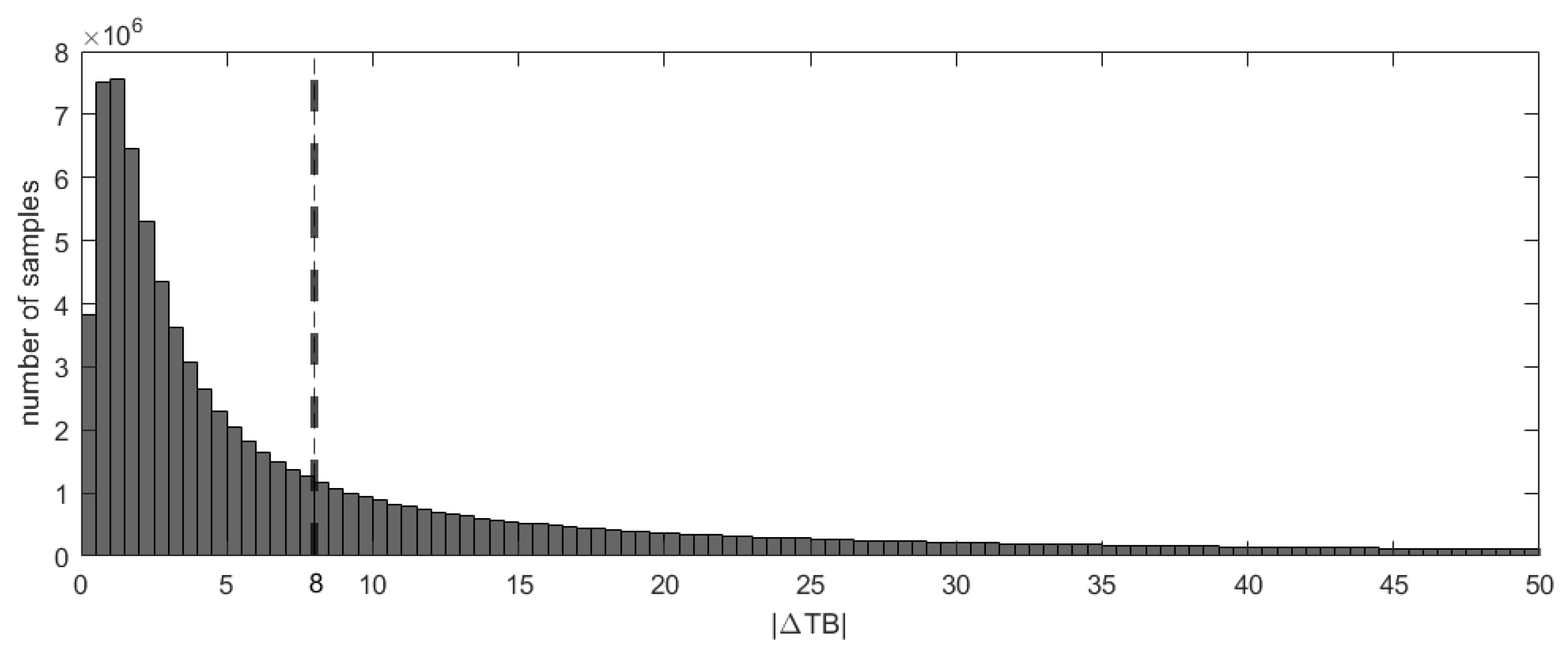
with γ a threshold brightness temperature square in terms of both | Δ T B i | (for instantaneous) and var ( Δ T B ) β (for the synoptic weather scale). By Equations (9) and (10), the new FT algorithm contains a synoptic time scales background to daily values as variance-based filtering. For example, sunny days will lead to Δ T B i γ     [33]; cloudy/slow winds days will be filtered out by       var ( Δ T B ) β γ 2 because these days do not last longer than the period of an atmospheric Rossby wave period in the middle latitudes. We calculate all | Δ T B i | from the grid inferred by SMAP FT products as the freeze state (Figure 2) and obtain γ = 8 K by statistically computing | Δ T B i | and var ( Δ T B ) β over the northern hemisphere to keep 95% confidence for cases where T 2 m < 0 °C. The bias of ERA-land–air temperature and collocated 0–7 cm soil temperature is about 1 K, which provides 95% ± 3% uncertainty [50]. Any day that can obtain | Δ T B i | from SMAP will be checked by Equation (10). For a day that | Δ T B i | is not available, it will be filled with an FT value depending on the nearest FTnew. In arid regions, Δ T B i γ     would always work because the heat capacity of dry soil is much smaller than that of wet soil. Equation (10) will treat the arid region as a thawed state. For wet snow, if there is no more water melted in the daytime, then TB will not be affected too much. If water is melting, Equation (10) will be treated as a thawed state, and the wet snow-covered ground will still be part of the land surface FT state.

2.3. Evaluation of the New FT-State Detection Algorithm

By Equation (10), one can compute the starting and ending times of the frozen-soil period in winter, i.e., the first/last freeze state in an annual FT cycle. Applying Equation (9), it requires at least one FT value per day which affects accuracy in the low latitudes.
Before a comparison with the half-daily SMAP FT products, we have to scale it to daily resolution by
F T   S M A P d a i l y = { t h a w ,         i f F T   s t a t u s 6 a m = 0         o r           F T   s t a t u s 6 p m = 0       f r o z e n ,       i f F T   s t a t u s 6 a m = F T   s t a t u s 6 p m = 1    
Equation (11) produces a bias towards thawed states but matches the concept of the new FT algorithm because | Δ T B i | would be smaller when the states at 6 a.m. and 6 p.m. are consistent. Hence, the agreement is defined as the fraction of days in which the new method and SMAP FT have the exact daily FT state inference against the total number of days (see Equation (11)). Specifically, both the SMAP’s FT product and the new algorithm contain 964 × 203 grids in the latitude between the equator to 83.6320°N and 2148 days after 31 March 2015. Instead, “agreement” computes the percentage of pairs (one from the new FT and the other from SMAP) that are consistent along longitude/latitude/time. SMAP also adopts a similar FT product-accuracy assessment method to Equation (11) [32]. The difference is that SMAP needs to compare at 6 a.m./pm instead of the daily scale.
With the above steps, the categorical triple collocation (CTC) method [51,52] is used for validating the binary FT state. Triple collocation (TC) is a method to verify the accuracy of three sets of observations without surface measurements. The method assumes the following relationship between the observed quantity (M) and the true value (X):
M i = A i + B i X + ε i
This method assumes that each group of observations is independent of the other and that observations and errors are separate. However, for binary variables (such as the freeze–thaw state of soil), Equation (12) should be rewritten as
M i = X + ε i
CTC is based on triple collocation (TC) [53,54] by relaxing the assumptions of TC sufficiently to allow its application to binary and categorical variables. CTC provides relative performance rankings but not absolute values of performance metrics.
The CTC method evaluates the estimation accuracy of binary variables by introducing equilibrium accuracy (α)
α i = 1 2 ( ψ i + η i )
In the formula, ψ is the probability of being correctly estimated as thawed, and η is the probability of being correctly estimated as frozen. The following relationship exists between the covariance matrix (Q) of the static variable and the equilibrium accuracy α,
Q i j = C o v ( M i , M j ) = { 1 E ( E ( M i ) ) 2 , f o r     i = j V a r ( X ) ( 2 α i 1 ) ( 2 α j 1 ) , f o r     i j
This relationship is extended to non-static variables with noticeable seasonal changes (such as a freeze–thaw state):
Q i j = C o v ( M i , M j ) = { 1 E ( E ( M i / t ) ) 2 , f o r     i = j 4 E ( p ( t ) ) ( 1 E ( p ( t ) ) ) ( 2 α i 1 ) ( 2 α j 1 ) , f o r     i j
In the formula p(t) ≡ pM (M = 1|t), t is time (unit is day). The CTC algorithm requires that the random errors between each group of observation systems are conditionally independent if the relative accuracy Wi is defined as
W i = 2 ( 2 α i 1 ) E ( p ( t ) ) ( 1 E ( p ( t ) ) )
Three groups of different observation systems in Equation (17) can form three equations, as follows:
W = [ Q 12 Q 13 Q 23 Q 12 Q 23 Q 13 Q 23 Q 13 Q 12 ]
Since Wi is a monotonically increasing function with αi as the independent variable, the ordering of W represents the ordering of the observation system errors from small to large. The relative error between different observation systems can be obtained by arranging the W vector calculated by Equation (18) in descending order [54].

3. Results

3.1. The Demonstration of the New Method at the Xilinhot Site

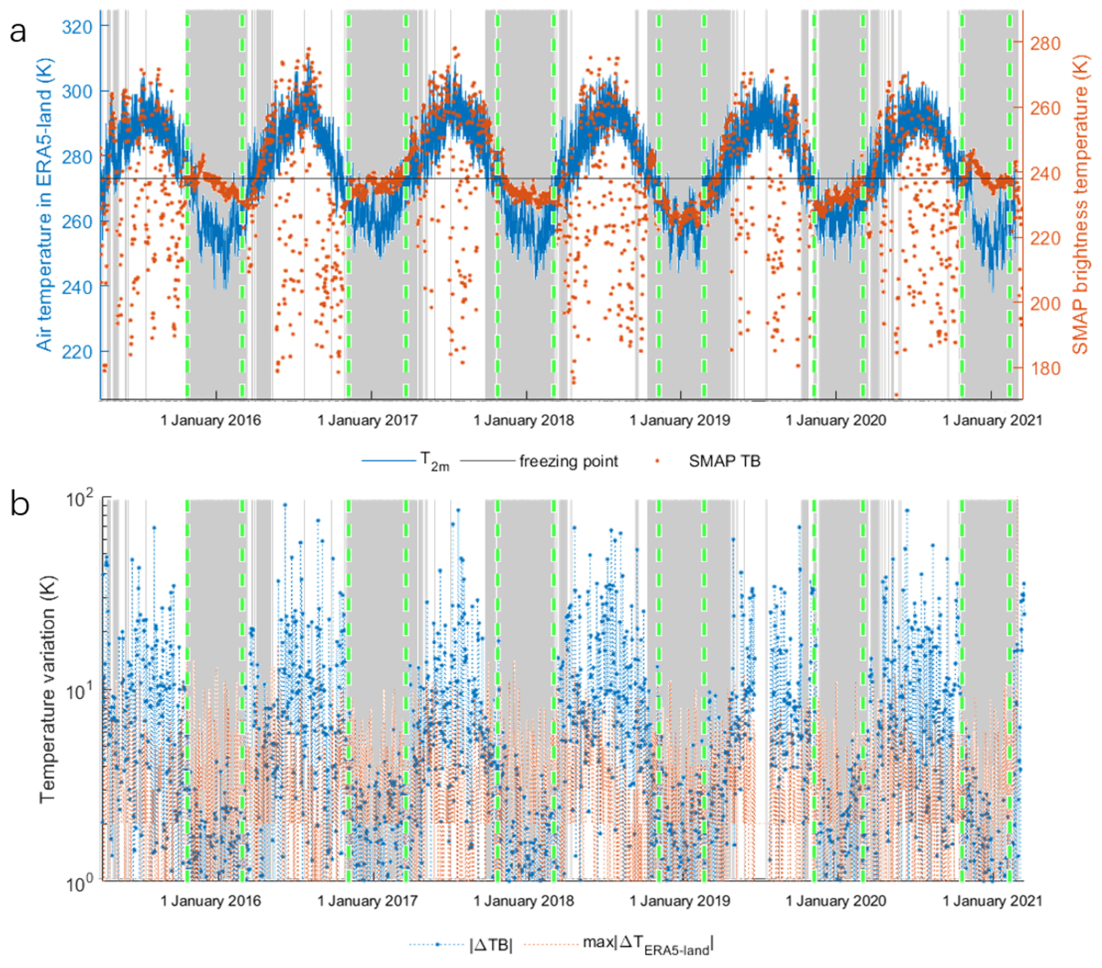
Figure 3a shows the in situ air temperatures and the SMAP TB observed at or near the Xilinhot site from March 2015 to March 2021. The green lines are the beginnings and ends of the annual freezing cycles inferred from the new FT algorithm. The intervals between green lines in summer indicate the thawed state, and in winter for the frozen state. TB ranges between 240 K and 280 K in the thawed soil state. The seasonal TB amplitude more or less follows the variation of air, skin, and upper soil temperatures without phase delay. Under frozen conditions, TB does not exhibit a clear seasonal variation because of a more stable soil emissivity. Figure 3b proves the inference from Equation (8): | Δ T s k i n | is the maximum difference between the 6 p.m. and 6 a.m. calculated from skin temperature (Tskin) in the ERA5-land (Figure 3a). | Δ T s k i n | is relatively stable, about 10–15 K through the years, while | Δ T B i | in winter is two times smaller than in summer.
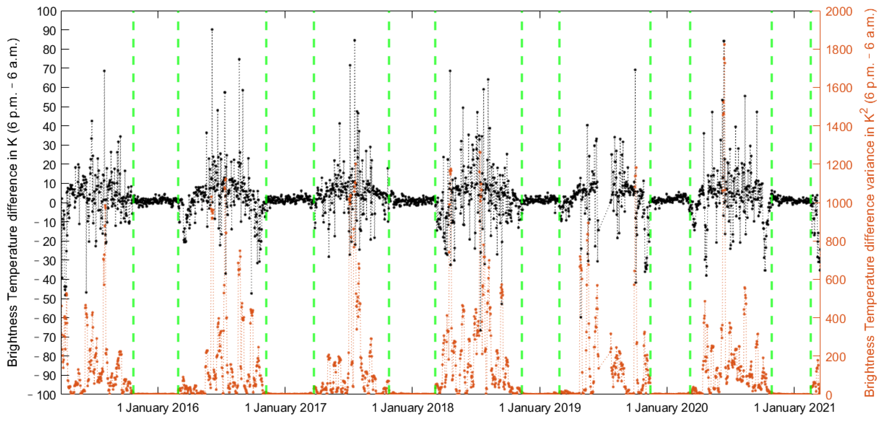
The ΔTBi time series in (Figure 4) shows mostly a substantial intra-annual variation in summer from −40 K to 40 K due to soil moisture variations, which is mainly influenced by the precipitation connected to the East Asia Monsoon. In winter, ΔTBi varies only from −8 K to 8 K. However, there are | Δ T B i | 8 K is summer as well. To filter out these isolated small | Δ T B i | cases in summer, var ( Δ T B ) β is constructed as in Equation (9). In Figure 4, var ( Δ T B ) β is close to zero but ranges from 0 to 200 K in summer. By comparison with ΔTBi, var ( Δ T B ) β = 7 (the red line in Figure 4) successfully filters out the small ΔTBi of summer cases. Figure 4 also shows the sudden changes of both ΔTBi and var ( Δ T B ) β = 7 in the beginning and ending time of the frozen-soil period according to the new algorithm.
At the beginning and after the end of an annual frozen-soil period (Figure 4), T B i h _ 6 p m is often less than T B i h _ 6 a m (valley in the time series), while the soil and air temperatures have opposite behavior due to solar heating during daylight hours. Days with T B i h _ 6 p m < T B i h _ 6 a m can be explained by daytime melting of the uppermost few centimeters of the soil, which reduces the topsoil emissivity. According to [55], intra-daily FT state transitions between the completely thawed and frozen-soil state may last for tens of days at the Maqu site on the Tibetan plateau [55]. The new FT detection algorithm takes this peculiarity during the transition phase into account and identifies the FT state of the bulk soil rather than of a thin surface layer as detected by the existing T B -based algorithms. Moreover, the new FT detection algorithm requires no local reference values.

3.2. Result over the Northern Hemisphere

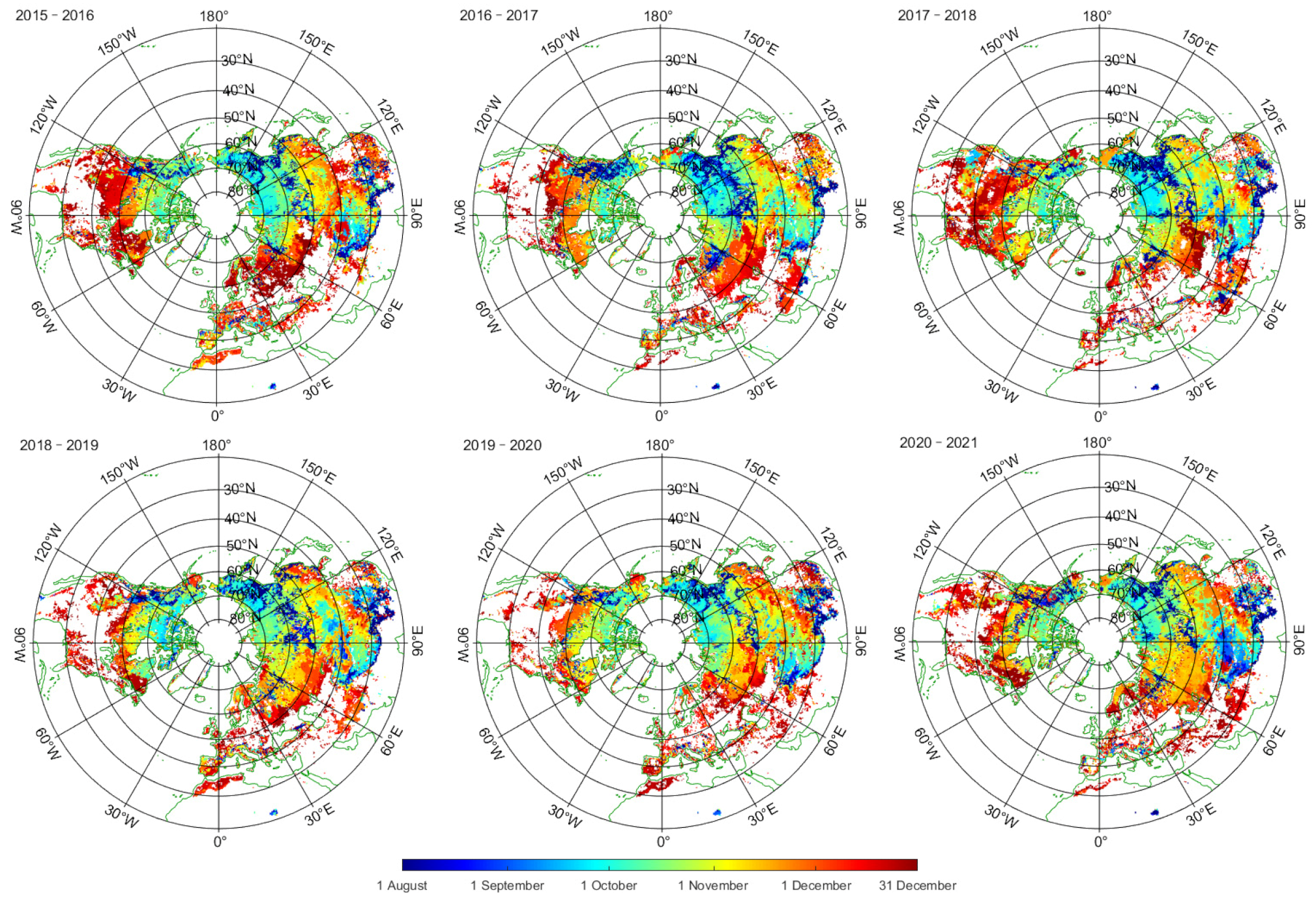
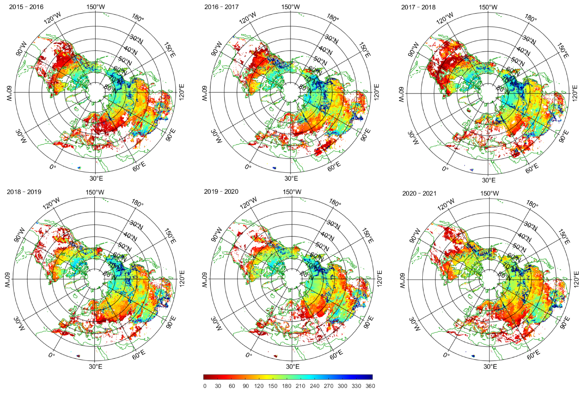
Figure 5 and Figure 6 show, respectively, the beginnings between August and December and the endings between January and May of the frozen-soil periods from 2015–2021. For most of the northern hemisphere, there are hardly any frozen-soil states in the northern hemisphere during June and July.
Siberia and Tibet experience the earliest soil freezing. In East Asia, the beginning of soil freezing follows the latitude and the East Asia Summer Monsoon [56] propagation in a meridional direction. Regions with an earlier retreat of the East Asia Summer Monsoon also freeze earlier, i.e., the region reaching from Mongolia to southern China shows a northwest–southeast freezing beginning gradient in November [57]. Over Europe, the gradient direction of the start times exhibits a southwest–northeast pattern towards Siberia. The freezing begins about two months later than in other regions with the same latitude (40°N~60°N) [58]. In North America, the freezing starts in October in the north and invades the south in December. Winter 2015–2016 and winter 2017–2018 show more severe soil freezing than other winters. Deep blue colors along 120°W mark the Rocky Mountains.
The pattern of the frozen-soil ending dates (Figure 6) is similar to the one of the starting dates. The frozen-soil period lasted the longest in Siberia, Tibet, and the Rocky Mountains. Winter 2017–2018 has the latest ending time of the frozen-soil period in North America and Europe. The contours of the frozen-soil period’s beginning vary by tens of days from year to year. Parts of Siberia and Tibet never have unfrozen soil (deep blue colors); the soils are also frozen during June and July, which are not shown in the figures. Color transitions in Figure 6 are smoother and more continuous than in Figure 5 and show a gentler date gradient. For instance, the gradient over Eurasia is spotted spatially in Figure 5. An air temperature drop may explain the jagged color contours in Figure 5. These delicate patterns reflecting topography, sea-land distribution, and climatological types are not observed in Figure 6, implying a more gradual and slower heating process in spring.
By combining Figure 5 and Figure 6, we obtain the duration of the annual frozen cycle as in Figure 7. The most extended frozen-soil period (>200 days) is located near the North Pole and over some regions in Tibet (Figure 7). The sharpest gradient in the length of the frozen period stretches from the eastern part of Siberia to the northeast part of China following the latitudes; here, the freezing duration decreases from more than 300 days to 90 days in about ten days per latitude degree. The freezing duration does not change much between the years and exhibits similar patterns.

3.3. The Comparison with the SMAP FT Products

In this section, we will compare the results from the new FT algorithm with SMAP’s regarding time variation and spatial distribution. An average of 2-m air temperature and collocated 0–7 cm soil temperature will also be used as a reference and compared with both FT results.
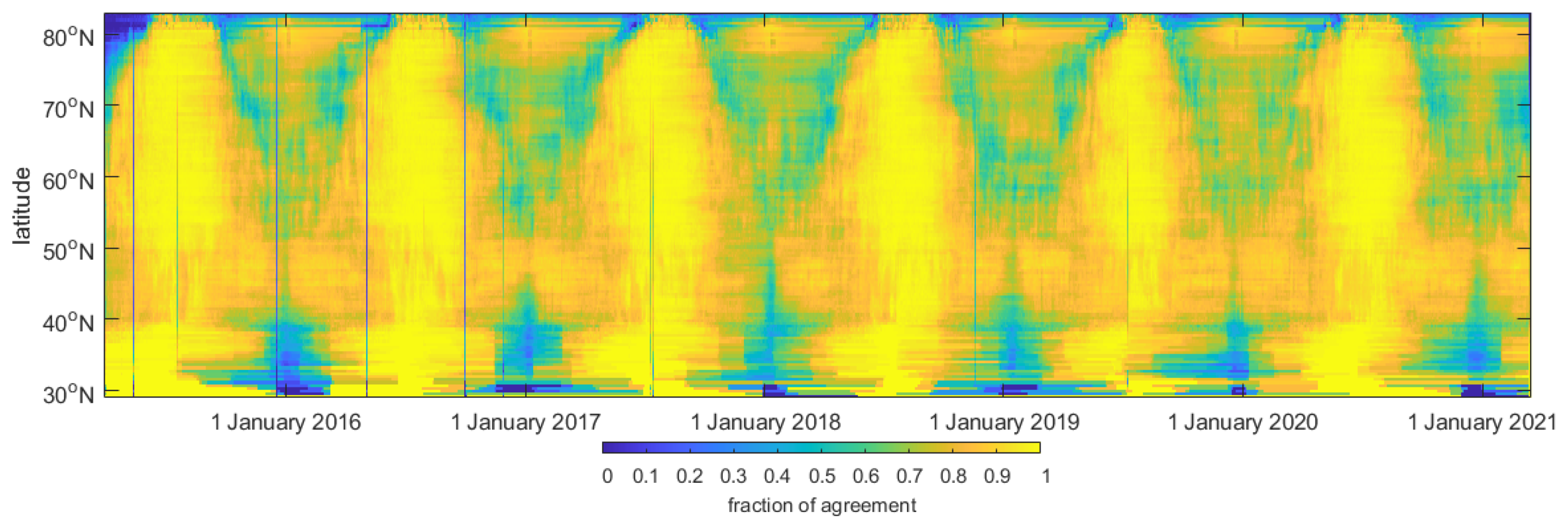
Figure 8 shows the zonal average agreement evolution along the annual FT transition zones between 30°N and 80°N. Although the SMAP FT product contains the data in 0°N–30°N, the zones that are supposed to be freeze-free or permanently frozen (>83°N) are not included in Figure 8. The new FT detection algorithm results mostly agree well with the SMAP FT product (Figure 8). In a transition zone, the overall agreement is only 0.6–0.7. The agreement of the detected beginning and ending times in the 30°N–40°N latitude belt is lower than the zones above 40°N because of the Tibet Plateau (25°N–40°N, see Figure 9a). The agreement between the two algorithms can be below 0.5 in winter (the blue area in Figure 8, especially ≥80°N).
In summer, both agree up to 0.98 and 0.70–0.75 in the wintertime. However, the lowest agreement does not happen in the deep winter but some time ahead and after January by showing the two valleys as seen for each year in Figure 8. These valleys are the freezing/thawing transition period in the northern hemisphere that obtains the lowest agreement.
The difference in Figure 8 is due to the hypothesis in both algorithms. The SMAP FT algorithm requires FFfr and FFth; their estimate needs sufficiently long periods of wet and frozen soil, which becomes increasingly difficult with decreasing latitude. Thus, FFfr and FFth can be unreliable for the transition zones where the frozen emission character is not typical and may have interannual changes. For instance, the FFfr and FFth change variation can reach 4% and 20%, respectively, and strongly depends on the samples. Table 1 illustrates FFfr and FFth variation at the Xilinhot site by adopting different samples every year. Another reason for the difference in Figure 8 is the assumption adopted by the new algorithm. For one side, the new algorithm cannot identify a frozen-soil period shorter than seven days (as shown in Equation (9)). This leads to the thawed/frozen error in the new FT algorithm where the 3–5 days heat/cold events may result in different FT states from the two algorithms.
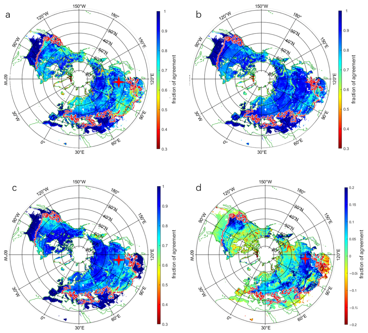
Figure 9a compares the SMAP FT state product and the new algorithm regarding the spatial distribution of the agreement. The Tibetan Plateau shows the lowest agreement value in Asia, especially its southern margin close to the Himalayas Mountains. While for most of the plateau, the agreement stays above 0.7, it is below 0.5 at some points organized in a belt in an east–west direction, probably due to the complex terrain that affects the ERA5-land quality [59]. The area downstream of the plateau, including the center parts of China, also shows strong disagreement between both estimates. A zone with a low agreement (0.7–0.8) is found between 50 and 60°N, especially in the Lake Baikal region, northern Europe, and the east coast of Canada and Alaska. A zone with high agreement is found in eastern China, central Asia, southwestern Europe, and the southern U.S. Figure 9b,c shows the same agreement map between the new/SMAP’s FT algorithm and the FT stated inferred from ERA-land-assessment data by a binary judgment of the freezing point (273.15 K), i.e., T < 273.15 K is frozen, and T > 273.15 K is thawed. Figure 9b,c shows that despite some mismatch between the results of the new algorithm and the SMAP FT, both overall agree by more than 70%. The new FT state detection better agrees with T2m in the mid-latitudes than the SMAP FT algorithm but is worse in latitudes above 60°N and low latitudes below 30°N. Figure 9c also shows the influence of SMAP’s NPR threshold method and the single channel algorithm with a clear boundary between high/low latitudes.
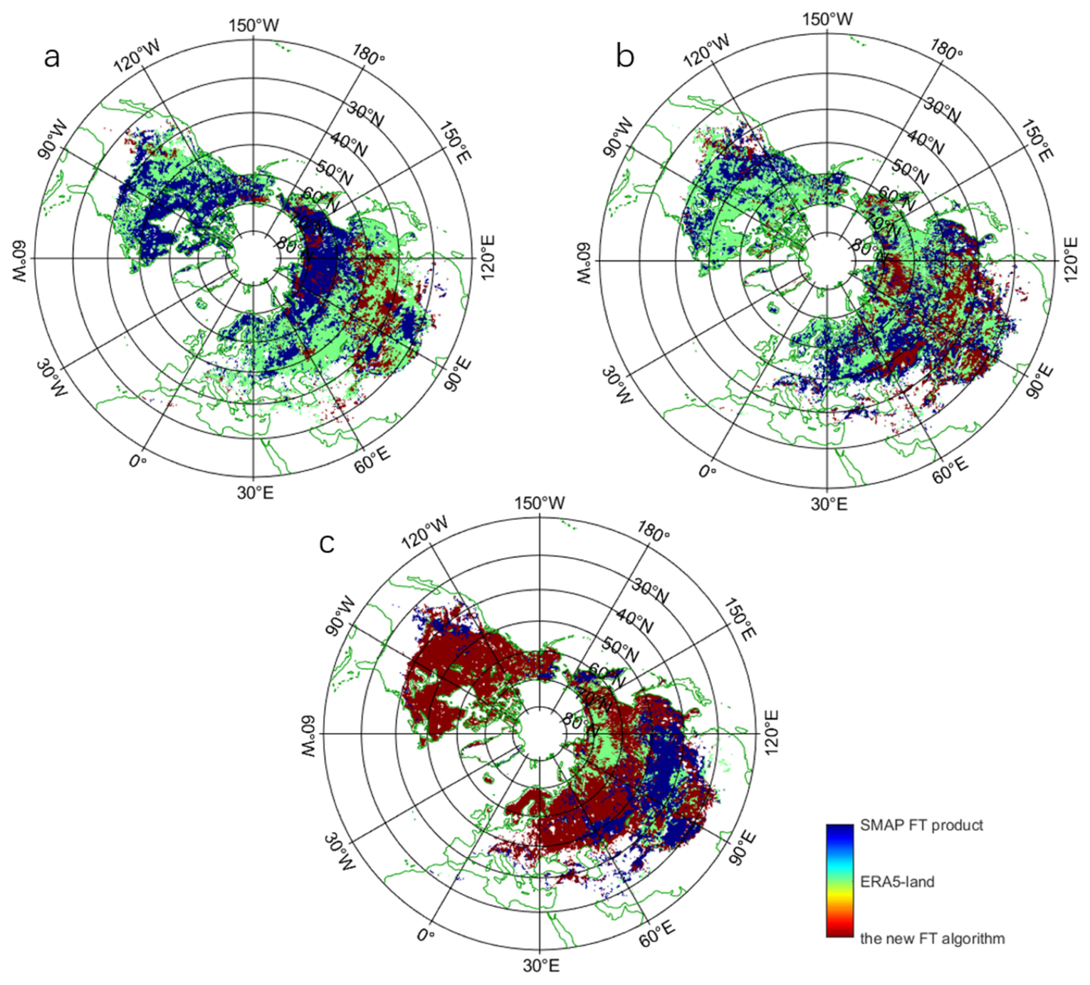
Figure 10 shows the CTC result, i.e., the new method F/T, ERA-land F/T, and SMAP F/T. SMAP F/T is confidently ranked the highest at high latitudes (≥60N°, Figure 10a). There are no dominant products that represent the FT state truth in the northern hemisphere in Rand Second (Figure 10c). However, for the mid-latitudes in East Asia, which includes the XInlinhot site, the new FT is more confident than SMAP’s FT product (Figure 10c).

3.4. Sensitivity Test

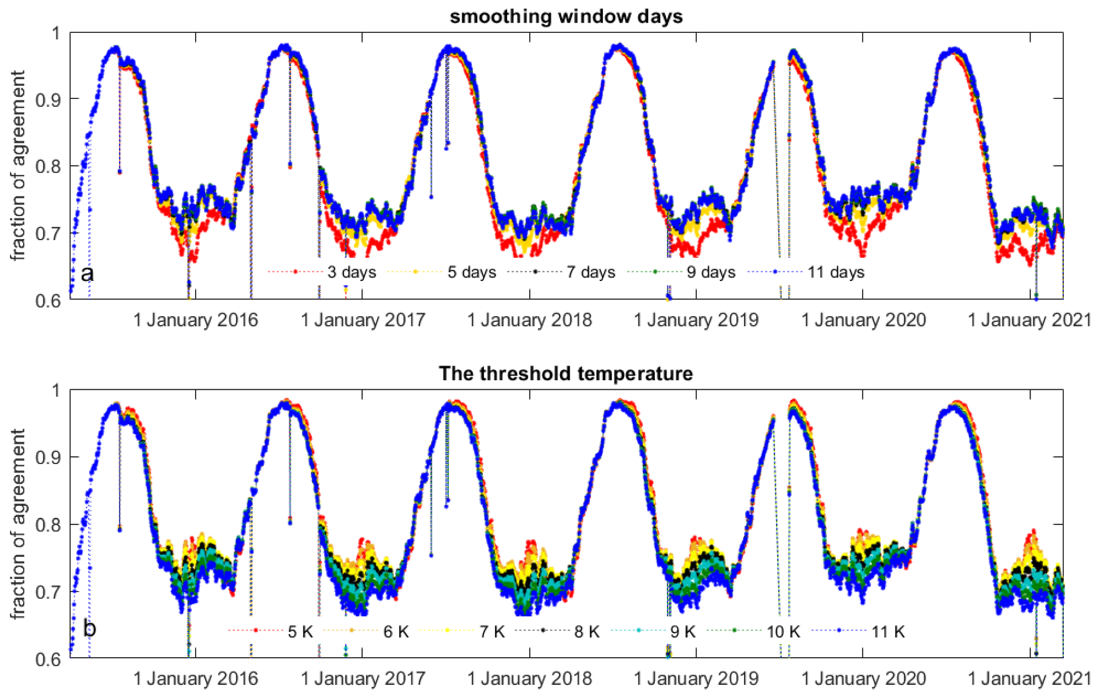
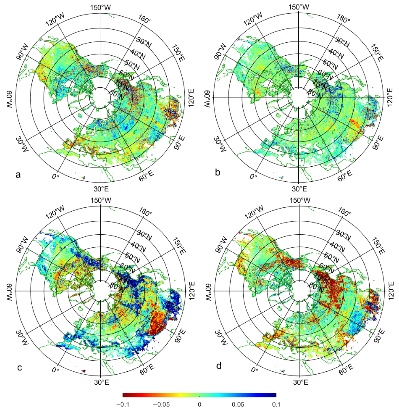
Parameters β and γ in the new FT state detection have been selected based on the typical length of synoptic weather systems and the 95% confidence level outcome. β (days) is the window length (days) over which the variance in Equation (9) is estimated and used as a decision criterium in Equation (11), which filters out sporadic changes by weather events. γ is a threshold temperature to judge if the observed SMAP TB signal is related to frozen soil in Equation (10). The values for these parameters have been set in an ad hoc fashion; here, we analyze the sensitivity of the results against the soil freeze/thaw state inferred from ERA-land-assessment data to the variation of these parameters by varying β from 5 to 11 K (Figure 11a and Figure 12a,b) and γ from 3 to 11 days (Figure 11b and Figure 12c,d).
When only changing one parameter, the degree of agreement between the new FT estimates and T2m changes significantly only in winter (Figure 11). The impact of changing only β is also larger in winter than in summer (Figure 11a). A smaller β reduces the agreement from above 0.73 (at β = 7) to 0.65 when β = 3, while a larger β only barely increases the agreement between both estimates. A smaller γ improves the agreement in winter (Figure 11b) by more than 0.1. Overall, the variation of the two parameters leads only to significant changes in the agreement between both estimates in the thawing period. The spatial distribution of the change of agreement between both FT state estimates relative to the default values for the two parameters is shown in Figure 12. The Tibetan Plateau and some Northern Europe areas behave opposite to Siberia, the western coast of North America, and the region around latitude 30°N.

4. Discussion

Although the result reveals the potential for retrieving the FT state from the DAV signals at the L band, several issues need to be addressed for further development as fellows,
The primary issue of the FT product-accuracy assessment of passive microwave remote sensing FT products is how to measure and define the FT on the ground, especially for a deeper penetrated band such as the L band. We lack a precise “ground truth” of the soil’s freeze/thaw state. The SMAP FT team uses WMO’s air temperature, and WMO’s air temperature is also vulnerable in the agreement assessment. For instance, what is the best way to deal with the scale mismatch between the weather station and SMAP’s footprint? How do we account for sub-grid open water fraction, terrain heterogeneity, tree cover, precipitation, snowmelt, and so on with the weather station data? These problems can be avoided by taking an average of ERA5-landland–air temperature and collocated 0–7 cm soil temperature in the evaluation, and we are aware that the ERA5-landland–air temperature and collocated 0–7 cm soil temperature are not appropriate for validation which needs FT ground profile truth for sure. ERA-land-assessment data FT inference is used in this study, and SMAP uses a more complicated scheme by considering T2m, Tskin, T5cm, and T10cm. Some studies use soil temperature to evaluate SMAP FT products, and with 0–5 cm, the soil temperature at SMAP grids containing CVS stations is about 70% [60]. Since in situ T2m is usually to either infer the ground FT states or those used in the FT products accuracy assessment, it is interesting to know the relationship between air temperature and FT state on a global scale. However, when it comes to soil temperatures such as Tskin, T5cm,, T10cm, or more profound layers, it is hard to say which layer can correspond to the TB signal best. Another option is in situ soil temperature at 5 cm, as in SMAP’s FT product-accuracy assessment. However, either the detectable depth or the footprint of SMAP’s radiometer does not match ERA5-land. Indeed, the soil temperature from a particular layer cannot compare with SMAP’s FT product because the penetration depth of the L-band signal is dynamic [61,62], especially for frozen soil that may range from a few centimeters to meters. Thus, the comparison in this study, such as Figure 9, Figure 10, Figure 11 and Figure 12, is hard to consider as an evaluation of the new FT algorithm or SMAP’s. Still, the comparison shows that the new FT algorithm can capture FT signals as well as the SMAP’s official one.
Since ERA-land-assessment data is adopted in this study, Figure 13 shows the frozen land cover and annual accumulations inferred from the new FT state algorithm and the thermal conditions near the surface from T2m < 273.15 K in the northern hemisphere. Both are very similar, while the maxima reached for both data sets are different due to their different grid sizes; SMAP data are given in area-equal grids 36 km in diameter (about 1300 km2), while ERA-land-assessment data used a 1° × 1° lat-lon grid (0 to 1000 km2). However, the frozen land area detected by the new FT algorithm is about 15 days in advance of T2m, especially in spring (the shift of black lines). It coincides with the challenges in using ERA-land-assessment data as an accuracy assessment for L-band-derived estimates of FT since the radiometer measurements are sensitive to the near-surface soil layer. The time lag in springs is reasonable because soil absorbs the solar radiation and then heats air temperature. The accumulated frozen land areas are also different. Usually, the air temperature will lead to more frozen soil flags, except for the year 2019. Figure 13 shows that T2m is also more appropriate to be the “ground truth” in the beginning than the ending of an annual FT cycle. A similar situation exists for Tskin, T5cm,, T10cm, or more profound layers. The penetration depth of the L-band detection varies severely during the FT transitions; thus, it would not be suitable to evaluate the FT algorithm with a static depth. Moreover, the penetration depth and sensing depth issues for soil moisture retrieving from L band are still unclear [28,62,63,64,65]. The problem is more complex for frozen soil because the dielectric profile is not continuous if freeze–thaw transitions happen in a profile’s middle layers, and a complete frozen soil profile shall theoretically have much deeper penetration. Thus, we cannot even get a precise penetration depth for the case of a freeze–thaw transition. By using the air temperature, we avoid this complicated situation. Otherwise, selecting which layer and according to what standard compared with the SMAP FT products would be vulnerable. In this study, we use the same method as the SMAP handbook, which is considered the state-of-art in this topic, to obtain the agreement.
Thus, clarifying the “ground truth” is critical to developing the FT remote sensing algorithm at the L band. Future work needs more in situ accuracy assessment activities in the field experiment, not only for the satellites but from tower-based or airborne platforms. The L-band TB detected by the satellites covers the FT states in tens of kilometers, and most importantly, the FT has a vertical structure. The field experiment is expected to identify the sensing depth, which is also a vague concept for soil moisture remote sensing at the L band during the FT transition periods. Instead, the ERA-land-assessment data makes the temporal and spatial scales more comparable with the FT result in this study. Specifically, (1) the vertical scale: the air temperature is a composite indicator of the FT state for a certain layer; (2) the temporal scale: the resolution of the DAV values is daily. It is reliable to use daily air temperature and collocated 0–7 cm soil temperature, not instant soil temperature, in the assessment.
Besides lacking appropriate ground truth, another limitation of the new algorithm is the absence of the DAV data in the low latitudes (≤45°N). The orbits of SMAP and SMOS make the revisit period over in the low latitudes more frequent than two times a day but only one value in 3 days. The new FT algorithm is based on a DAV signal as in Equation (8) and further extends to the synoptic scale by the parameter β. Thus, a lot of data are absent in the low latitudes area. To overcome this drawback, we have to define the annual FT scale’s beginning and ending times and fill the DAV absence with the nearest interpolation. This produces dummy signals that affect the accuracy in low latitudes. In all cases, the daily L3_FT products incorporate (AM and PM satellite overpasses) data for the current day, as well as past days’ information (to a maximum of 3 days, necessary only near the southern margin of the FT domain) to ensure complete coverage of the FT domain in each day’s product.

5. Conclusions

We developed a new FT state-detection algorithm based on the difference in the microwave brightness temperature between 6 a.m. descending and 6 p.m. ascending half-orbit passes that are relatively small over frozen soil due to the large penetration depth leading to an effective temperature dominated by stable deeper soil temperatures. The new FT state detection agrees well with SMAP’s FT state detection, with a minimum of above 0.72 in winter. The new algorithm can reach a comparable agreement regarding the spatial distribution as the SMAP FT product does against ERA-land-assessment data FT inference in the northern hemisphere. The algorithm is rather stable to variations of its ad hoc set parameters. The limitation is that this algorithm is only applicable to the L band, considering its penetration depth and corresponding soil effective temperatures; it cannot be applied to other bands. The new algorithm presented in this study is expected to extend the application of L-band passive microwave remote sensing data in freezing-thawing conditions.
Since the sensitivity of the L-band signal to the F/T state varies in terms of land cover type and climate regions, the new algorithm shall be validated with in-site FT observations at various sites. For instance, the sub-grid open-water fraction, tree cover, precipitation, and snowmelt critical to TB signals at the L band shall be checked. These dynamics will enlarge/reduce the DAV signals and further the efficiency of parameters β and γ. On the other hand, the terrain is a significant factor because we can see Tibet and the Rocky Mountains in Figure 9. Although the new algorithm shows comparable agreement with SMAP’s FT products, further optimization, and validation work, should be carried out in the future.

Author Contributions

Data curation, Y.Z., Y.G. and Z.S.; Formal analysis, J.W.; Funding acquisition, C.S.; Writing—original draft, S.L. All authors have read and agreed to the published version of the manuscript.

Funding

This research was funded by the National Natural Science Foundation of China (Grant 42075150); by the Natural Science Foundation of Shanghai (No. 21ZR1405500); and by the Deutsche Forschungsgemeinschaft (DFG) via the research group FOR2131 on “Data Assimilation for Improved Characterization of Fluxes across Compartmental Interfaces”, subproject P2.

Data Availability Statement

Conflicts of Interest

The authors declare no conflict of interest.

References

  1. Walvoord, M.A.; Kurylyk, B.L. Hydrologic Impacts of Thawing Permafrost-A Review. Vadose Zone J. 2016, 15, 1–20. [Google Scholar] [CrossRef]
  2. Schuur, E.A.G.; McGuire, A.D.; Schädel, C.; Grosse, G.; Harden, J.W.; Hayes, D.J.; Hugelius, G.; Koven, C.D.; Kuhry, P.; Lawrence, D.M.; et al. Climate change and the permafrost carbon feedback. Nature 2015, 520, 171–179. [Google Scholar] [CrossRef]
  3. Zeng, Y.; Su, Z.; Barmpadimos, I.; Perrels, A.; Poli, P.; Boersma, K.F.; Frey, A.; Ma, X.; de Bruin, K.; Goosen, H.; et al. Towards a Traceable Climate Service: Assessment of Quality and Usability of Essential Climate Variables. Remote Sens. 2019, 11, 1186. [Google Scholar] [CrossRef]
  4. Yu, L.; Fatichi, S.; Zeng, Y.; Su, Z. The role of vadose zone physics in the ecohydrological response of a Tibetan meadow to freeze-thaw cycles. Cryosphere 2020, 14, 4653–4673. [Google Scholar] [CrossRef]
  5. Hu, G.; Zhao, L.; Wu, X.; Li, R.; Wu, T.; Xie, C.; Pang, Q.; Zou, D. Comparison of the thermal conductivity parameterizations for a freeze-thaw algorithm with a multi-layered soil in permafrost regions. CATENA 2017, 156, 244–251. [Google Scholar] [CrossRef]
  6. Gao, J.Q.; Xie, Z.H.; Wang, A.W.; Luo, Z.D. Numerical simulation based on two-directional freeze and thaw algorithm for thermal diffusion model. Appl. Math. Mech.-Engl. 2016, 37, 1467–1478. [Google Scholar] [CrossRef]
  7. Zhao, T.; Shi, J.; Hu, T.; Zhao, L.; Zou, D.; Wang, T.; Ji, D.; Li, R.; Wang, P. Estimation of high-resolution near-surface freeze/thaw state by the integration of microwave and thermal infrared remote sensing data on the Tibetan Plateau. Earth Space Sci. 2017, 4, 472–484. [Google Scholar] [CrossRef]
  8. Koven, C.D.; Ringeval, B.; Friedlingstein, P.; Ciais, P.; Cadule, P.; Khvorostyanov, D.; Krinner, G.; Tarnocai, C. Permafrost carbon-climate feedbacks accelerate global warming. Proc. Natl. Acad. Sci. USA 2011, 108, 14769–14774. [Google Scholar] [CrossRef]
  9. Koven, C.D.; Riley, W.J.; Stern, A. Analysis of Permafrost Thermal Dynamics and Response to Climate Change in the CMIP5 Earth System Models. J. Clim. 2013, 26, 1877–1900. [Google Scholar] [CrossRef]
  10. Zhao, P.; Xu, X.; Chen, F.; Guo, X.; Zheng, X.; Liu, L.; Hong, Y.; Li, Y.; La, Z.; Peng, H.; et al. The Third Atmospheric Scientific Experiment for Understanding the Earth-Atmosphere Coupled System over the Tibetan Plateau and Its Effects. Bull. Am. Meteorol. Soc. 2018, 99, 757–776. [Google Scholar] [CrossRef]
  11. Kimball, J.S.; White, M.A.; Running, S.W. BIOME-BGC simulations of stand hydrologic processes for BOREAS. J. Geophys. Res. -Atmos. 1997, 102, 29043–29051. [Google Scholar] [CrossRef]
  12. Li, F.Y.; Newton, P.C.D.; Lieffering, M. Testing simulations of intra- and inter-annual variation in the plant production response to elevated CO2 against measurements from an 11-year FACE experiment on grazed pasture. Glob. Chang. Biol. 2014, 20, 228–239. [Google Scholar] [CrossRef] [PubMed]
  13. Cramer, W.; Kicklighter, D.W.; Bondeau, A.; Iii, B.M.; Churkina, G.; Nemry, B.; Ruimy, A.; Schloss, A.L.; Participants Potsdam, N.P.P.M.I. Comparing global models of terrestrial net primary productivity (NPP): Overview and key results. Glob. Chang. Biol. 1999, 5, 1–15. [Google Scholar] [CrossRef]
  14. Matzner, E.; Borken, W. Do freeze-thaw events enhance C and N losses from soils of different ecosystems? A review. Eur. J. Soil Sci. 2008, 59, 274–284. [Google Scholar] [CrossRef]
  15. Wang, S.; Zhang, Y.; Lu, S.; Su, P.; Shang, L.; Li, Z. Biophysical regulation of carbon fluxes over an alpine meadow ecosystem in the eastern Tibetan Plateau. Int. J. Biometeorol. 2016, 60, 801–812. [Google Scholar] [CrossRef] [PubMed]
  16. Xie, Z.H.; Liu, S.; Zeng, Y.J.; Gao, J.Q.; Qin, P.H.; Jia, B.H.; Xie, J.B.; Liu, B.; Li, R.C.; Wang, Y.; et al. A High-Resolution Land Model With Groundwater Lateral Flow, Water Use, and Soil Freeze-Thaw Front Dynamics and its Application in an Endorheic Basin. J. Geophys. Res. -Atmos. 2018, 123, 7204–7222. [Google Scholar] [CrossRef]
  17. Swenson, S.C.; Lawrence, D.; Lee, H. Improved simulation of the terrestrial hydrological cycle in permafrost regions by the Community Land Model. J. Adv. Modeling Earth Syst. 2012, 4, M08002. [Google Scholar] [CrossRef]
  18. Yu, L.; Zeng, Y.; Su, Z. Understanding the mass, momentum, and energy transfer in the frozen soil with three levels of model complexities. Hydrol. Earth Syst. Sci. 2020, 24, 4813–4830. [Google Scholar] [CrossRef]
  19. Yu, L.Y.; Zeng, Y.J.; Wen, J.; Su, Z.B. Liquid-Vapor-Air Flow in the Frozen Soil. J. Geophys. Res. -Atmos. 2018, 123, 7393–7415. [Google Scholar] [CrossRef]
  20. Mwangi, S.; Zeng, Y.; Montzka, C.; Yu, L.; Su, Z. Assimilation of Cosmic-Ray Neutron Counts for the Estimation of Soil Ice Content on the Eastern Tibetan Plateau. J. Geophys. Res. -Atmos. 2020, 125, e2019JD031529. [Google Scholar] [CrossRef] [Green Version]
  21. Yashchenko, A.S.; Bobrov, P.P. Impact of the Soil Moisture Distribution in the Top Layer on the Accuracy Moisture Retrieval by Microwave Radiometer Data. IEEE Trans. Geosci. Remote Sens. 2016, 54, 5239–5246. [Google Scholar] [CrossRef]
  22. Schwank, M.; Stahli, M.; Wydler, H.; Leuenberger, J.; Matzler, C.; Fluhler, H. Microwave L-band emission of freezing soil. IEEE Trans. Geosci. Remote Sens. 2004, 42, 1252–1261. [Google Scholar] [CrossRef]
  23. Rautiainen, K.; Lemmetyinen, J.; Schwank, M.; Kontu, A.; Ménard, C.B.; Mätzler, C.; Drusch, M.; Wiesmann, A.; Ikonen, J.; Pulliainen, J. Detection of soil freezing from L-band passive microwave observations. Remote Sens. Environ. 2014, 147, 206–218. [Google Scholar] [CrossRef]
  24. Kim, Y.; Kimball, J.S.; Glassy, J.; McDonald, K.C. MEaSUREs Global Record of Daily Landscape Freeze/Thaw Status, Version 4 [dataset]. 2017. [Google Scholar] [CrossRef]
  25. Kim, Y.; Kimball, J.S.; McDonald, K.C.; Glassy, J. Developing a Global Data Record of Daily Landscape Freeze/Thaw Status Using Satellite Passive Microwave Remote Sensing. IEEE Trans. Geosci. Remote Sens. 2011, 49, 949–960. [Google Scholar] [CrossRef]
  26. Xu, X.; Dunbar, R.; Derksen, C.; Colliander, A.; Kim, Y.; Kimball, J. SMAP L3 Radiometer Global and Northern Hemisphere Daily 36 km EASE-Grid Freeze/Thaw State, Version 3, Thaw State, Version, 3. 2020. Available online: https://nsidc.org/data/spl3ftp/versions/2 (accessed on 1 May 2020).
  27. Rautiainen, K.; Parkkinen, T.; Lemmetyinen, J.; Schwank, M.; Wiesmann, A.; Ikonen, J.; Derksen, C.; Davydov, S.; Davydova, A.; Boike, J.; et al. SMOS prototype algorithm for detecting autumn soil freezing. Remote Sens. Environ. 2016, 180, 346–360. [Google Scholar] [CrossRef]
  28. Lv, S.; Zeng, Y.; Su, Z.; Wen, J. A Closed-Form Expression of Soil Temperature Sensing Depth at L-Band. IEEE Trans. Geosci. Remote Sens. 2019, 57, 4889–4897. [Google Scholar] [CrossRef]
  29. Zhao, T.; Shi, J.; Zhao, S.; Chen, K.; Wang, P.; Li, S.; Xiong, C.; Xiao, Q. Measurement and Modeling of Multi-Frequency Microwave Emission of Soil Freezing and Thawing Processes. In Proceedings of the 2018 Progress in Electromagnetics Research Symposium (PIERS-Toyama), Toyama, Japan, 1–4 August 2018; pp. 31–36. [Google Scholar] [CrossRef]
  30. Lv, S.; Zeng, Y.; Wen, J.; Zhao, H.; Su, Z. Estimation of Penetration Depth from Soil Effective Temperature in Microwave Radiometry. Remote Sens. 2018, 10, 519. [Google Scholar] [CrossRef]
  31. Kim, Y.; Kimball, J.S.; Glassy, J.; Du, J.Y. An extended global Earth system data record on daily landscape freeze-thaw status determined from satellite passive microwave remote sensing. Earth Syst. Sci. Data 2017, 9, 133–147. [Google Scholar] [CrossRef] [Green Version]
  32. Dunbar, S.; Xu, X.; Colliander, A.; Derksen, C.; Kimball, J.; Kim, Y. Algorithm Theoretical Basis Document (ATBD). SMAP Level 3 Radiometer Freeze/Thaw Data Products. JPL CIT JPL 2020, 500, 33. [Google Scholar]
  33. Sharifnezhad, Z.; Norouzi, H.; Prakash, S.; Blake, R.; Khanbilvardi, R. Diurnal Cycle of Passive Microwave Brightness Temperatures over Land at a Global Scale. Remote Sens. 2021, 13, 817. [Google Scholar] [CrossRef]
  34. Kopczynski, S.; Ramage, J.; Lawson, D.; Goetz, S.; Evenson, E.; Denner, J.; Larson, G. Passive microwave (SSM/I) satellite predictions of valley glacier hydrology, Matanuska Glacier, Alaska. Geophys. Res. Lett. 2008, 35, 2008GL034615. [Google Scholar] [CrossRef]
  35. Tedesco, M. Snowmelt detection over the Greenland ice sheet from SSM/I brightness temperature daily variations. Geophys. Res. Lett. 2007, 34, 2006GL028466. [Google Scholar] [CrossRef]
  36. Guo, D.; Wang, H. Simulated change in the near-surface soil freeze/thaw cycle on the Tibetan Plateau from 1981 to 2010. Chin. Sci. Bull. 2014, 59, 2439–2448. [Google Scholar] [CrossRef]
  37. Chaubell, J.; Yueh, S.; Entekhabi, D.; Peng, J. Resolution enhancement of SMAP radiometer data using the Backus Gilbert optimum interpolation technique. In Proceedings of the 2016 IEEE International Geoscience and Remote Sensing Symposium (IGARSS), Beijing, China, 10–15 July 2016; pp. 284–287. [Google Scholar] [CrossRef]
  38. Muñoz-Sabater, J.; Dutra, E.; Agustí-Panareda, A.; Albergel, C.; Arduini, G.; Balsamo, G.; Boussetta, S.; Choulga, M.; Harrigan, S.; Hersbach, H.; et al. ERA5-Land: A state-of-the-art global reanalysis dataset for land applications. Earth Syst. Sci. Data Discuss 2021, 13, 4349–4383. [Google Scholar] [CrossRef]
  39. Baker, D.G.; Ruschy, D.L. Calculated and Measured Air and Soil Freeze-Thaw Frequencies. J. Appl. Meteorol. Climatol. 1995, 34, 2197–2205. [Google Scholar] [CrossRef]
  40. Fortin, G. Variability and frequency of the freeze thaw cycles in Quebec region, 1977-2006. Can. Geogr. -Geogr. Can. 2010, 54, 196–208. [Google Scholar] [CrossRef]
  41. Ho, E.; Gough, W.A. Freeze thaw cycles in Toronto, Canada in a changing climate. Theor. Appl. Climatol. 2006, 83, 203–210. [Google Scholar] [CrossRef]
  42. Zhao, T.; Shi, J.; Entekhabi, D.; Jackson, T.J.; Hu, L.; Peng, Z.; Yao, P.; Li, S.; Kang, C.S. Retrievals of soil moisture and vegetation optical depth using a multi-channel collaborative algorithm. Remote Sens. Environ. 2021, 257, 112321. [Google Scholar] [CrossRef]
  43. Yamano, H.; Chen, J.; Tamura, M. Hyperspectral identification of grassland vegetation in Xilinhot, Inner Mongolia, China. Int. J. Remote Sens. 2003, 24, 3171–3178. [Google Scholar] [CrossRef]
  44. Shi, C.X.; Xie, Z.H.; Qian, H.; Liang, M.L.; Yang, X.C. China land soil moisture EnKF data assimilation based on satellite remote sensing data. Sci. China-Earth Sci. 2011, 54, 1430–1440. [Google Scholar] [CrossRef]
  45. Wu, S.; Chen, J. Validation of AMSR-E soil moisture products in Xilinhot grassland. In Proceedings of the Remote Sensing for Agriculture, Ecosystems, and Hydrology XIV, Edinburgh, UK, 24–26 September 2012; p. 85311J. [Google Scholar]
  46. Chapin, F.S.; Sala, O.E.; Huber-Sannwald, E. Global Biodiversity in a Changing Environment: Scenarios for the 21st Century; Springer Science & Business Media: Berlin/Heidelberg, Germany, 2013. [Google Scholar]
  47. Derksen, C.; Xu, X.L.; Dunbar, R.S.; Colliander, A.; Kim, Y.; Kimball, J.S.; Black, T.A.; Euskirchen, E.; Langlois, A.; Loranty, M.M.; et al. Retrieving landscape freeze/thaw state from Soil Moisture Active Passive (SNAP) radar and radiometer measurements. Remote Sens. Environ. 2017, 194, 48–62. [Google Scholar] [CrossRef]
  48. Lv, S.; Zeng, Y.; Wen, J.; Zheng, D.; Su, Z. Determination of the Optimal Mounting Depth for Calculating Effective Soil Temperature at L-Band: Maqu Case. Remote Sens. 2016, 8, 476. [Google Scholar] [CrossRef]
  49. Blackmon, M.L. A Climatological Spectral Study of the 500 mb Geopotential Height of the Northern Hemisphere. J. Atmos. Sci. 1976, 33, 1607–1623. [Google Scholar] [CrossRef]
  50. Cao, B.; Gruber, S.; Zheng, D.; Li, X. The ERA5-Land soil temperature bias in permafrost regions. Cryosphere 2020, 14, 2581–2595. [Google Scholar] [CrossRef]
  51. McColl, K.A.; Roy, A.; Derksen, C.; Konings, A.; Alemohammad, S.H.; Entekhabi, D. Triple collocation for binary and categorical variables: Application to validating landscape freeze/thaw retrievals. Remote Sens. Environ. 2016, 176, 31–42. [Google Scholar] [CrossRef]
  52. Scott, K.A. Assessment of Categorical Triple Collocation for Sea Ice/Open Water Observations: Application to the Gulf of Saint Lawrence. IEEE Trans. Geosci. Remote Sens. 2019, 57, 9659–9673. [Google Scholar] [CrossRef]
  53. Stoffelen, A. Toward the true near-surface wind speed: Error modeling and calibration using triple collocation. J. Geophys. Res. Ocean. 1998, 103, 7755–7766. [Google Scholar] [CrossRef]
  54. Li, H.; Chai, L.; Crow, W.; Dong, J.; Liu, S.; Zhao, S. The reliability of categorical triple collocation for evaluating soil freeze/thaw datasets. Remote Sens. Environ. 2022, 281, 113240. [Google Scholar] [CrossRef]
  55. Su, Z.; Wen, J.; Zeng, Y.; Zhao, H.; Lv, S.; Van Der Velde, R.; Zheng, D.; Wang, X.; Wang, Z.; Schwank, M.; et al. Multiyear in-situ L-band microwave radiometry of land surface processes on the Tibetan Plateau. Sci. Data 2020, 7, 317. [Google Scholar] [CrossRef]
  56. Wang, B.; Ho, L.; Zhang, Y.; Lu, M.-M. Definition of South China Sea monsoon onset and commencement of the East Asia summer monsoon. J. Clim. 2004, 17, 699–710. [Google Scholar] [CrossRef]
  57. Cai, M.; Ren, R.C. Meridional and downward propagation of atmospheric circulation anomalies. Part I: Northern Hemisphere cold season variability. J. Atmos Sci. 2007, 64, 1880–1901. [Google Scholar] [CrossRef]
  58. Harris, C.; Arenson, L.U.; Christiansen, H.H.; Etzemuller, B.; Frauenfelder, R.; Gruber, S.; Haeberli, W.; Hauck, C.; Holzle, M.; Humlum, O.; et al. Permafrost and climate in Europe: Monitoring and modelling thermal, geomorphological and geotechnical responses. Earth-Sci. Rev. 2009, 92, 117–171. [Google Scholar] [CrossRef]
  59. Huang, X.; Han, S.; Shi, C. Multiscale Assessments of Three Reanalysis Temperature Data Systems over China. Agriculture 2021, 11, 1292. [Google Scholar] [CrossRef]
  60. Kraatz, S.; Jacobs, J.M.; Schröder, R.; Cho, E.; Cosh, M.; Seyfried, M.; Prueger, J.; Livingston, S. Evaluation of SMAP Freeze/Thaw Retrieval Accuracy at Core Validation Sites in the Contiguous United States. Remote Sens. 2018, 10, 1483. [Google Scholar] [CrossRef]
  61. Zheng, D.; Li, X.; Zhao, T.; Wen, J.; van der Velde, R.; Schwank, M.; Wang, X.; Wang, Z.; Su, Z. Impact of Soil Permittivity and Temperature Profile on L-Band Microwave Emission of Frozen Soil. IEEE Trans. Geosci. Remote Sens. 2020, 59, 4080–4093. [Google Scholar] [CrossRef]
  62. Zheng, D.; Li, X.; Wang, X.; Wang, Z.; Wen, J.; van der Velde, R.; Schwank, M.; Su, Z. Sampling depth of L-band radiometer measurements of soil moisture and freeze-thaw dynamics on the Tibetan Plateau. Remote Sens. Environ. 2019, 226, 16–25. [Google Scholar] [CrossRef]
  63. Roy, A.; Toose, P.; Williamson, M.; Rowlandson, T.; Derksen, C.; Royer, A.; Berg, A.A.; Lemmetyinen, J.; Arnold, L. Response of L-Band brightness temperatures to freeze/thaw and snow dynamics in a prairie environment from ground-based radiometer measurements. Remote Sens. Environ. 2017, 191, 67–80. [Google Scholar] [CrossRef]
  64. Rowlandson, T.L.; Berg, A.A.; Roy, A.; Kim, E.; Lara, R.P.; Powers, J.; Lewis, K.; Houser, P.; McDonald, K.; Toose, P.; et al. Capturing agricultural soil freeze/thaw state through remote sensing and ground observations: A soil freeze/thaw validation campaign. Remote Sens. Environ. 2018, 211, 59–70. [Google Scholar] [CrossRef]
  65. Wang, J.; Jiang, L.; Cui, H.; Wang, G.; Yang, J.; Liu, X.; Su, X. Evaluation and analysis of SMAP, AMSR2 and MEaSUREs freeze/thaw products in China. Remote Sens. Environ. 2020, 242, 111734. [Google Scholar] [CrossRef]
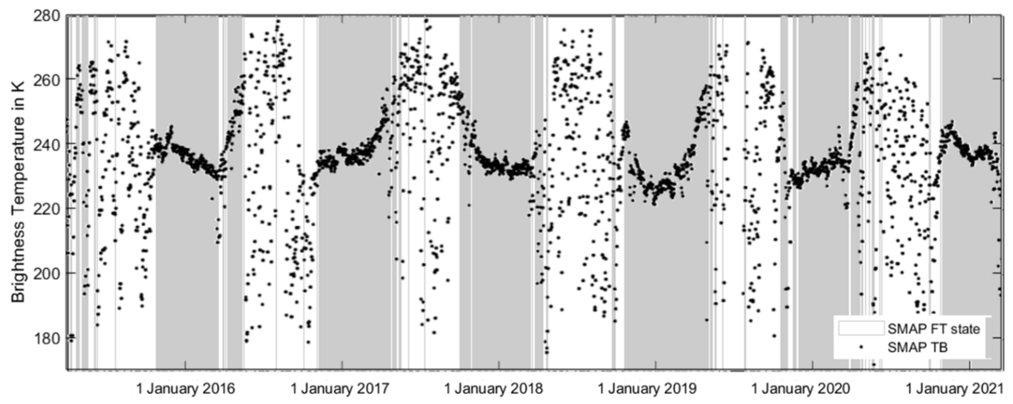
Figure 1. SMAP H-polarization TB time series and the derived reference FT state (grey for frozen and white for unfrozen) extracted for the location of the Xilinhot site (43°30’–45°N, 115°–117°E).
Remotesensing 14 04747 g001
Figure 2. | Δ T B | with β = 7 by SMAP TB data contained in SMAP L3 radiometer global daily 36 km EASE-grid freeze/thaw state; data over the northern hemisphere where 95% of samples are within 8 K.
Remotesensing 14 04747 g002
Figure 3. (a) Time-series of 2-meter air temperature T 2 m , and SMAP T B at the Xilinhot site; (b) time series of | Δ T B | computed from the SMAP TBs and max | ( Δ T E R A 5 l a n d ) | . The vertical green dashed lines indicate the beginning and ending day of the soil frozen state as inferred from the new FT algorithm. The gray shades the frozen state inferred from SMAP FT product.
Remotesensing 14 04747 g003
Figure 4. An illustration of diagnosis example at the Xilinhot site. The time series of ΔTB (Equation (7)) is represented by the black line from April 2015 to March 2021. The red line represents its seven-day moving variance as in Equation (9). The green dashed lines represent the beginning/ending of the soil frozen state inferred from the new FT algorithm.
Remotesensing 14 04747 g004
Figure 5. The beginning of the frozen-soil periods of the six winters as inferred by the new FT algorithm over the northern hemisphere (latitude > 20°N).
Remotesensing 14 04747 g005
Figure 6. The ending of the frozen-soil periods of the six winters as inferred by the new FT algorithm.
Remotesensing 14 04747 g006
Figure 7. The duration of the frozen period inferred from the SMAP L3 global H-polarization brightness temperature product.
Remotesensing 14 04747 g007
Figure 8. The fraction of agreement time series along the latitudes.
Remotesensing 14 04747 g008
Figure 9. The spatial pattern of the fraction of agreement in the northern hemisphere between (a) the new method and SMAP L3 FT state products; (b) the new method and ERA-land-assessment data; (c) the SMAP L3 FT state products and ERA-land-assessment data; and (d) the difference by b minus c. The red cross marks the location of Xilinhot, and the red line is the boundary between SMAP’s NPR threshold method and the single channel algorithm.
Remotesensing 14 04747 g009
Figure 10. Map of the measurement system ranked first (a), second (b), and third (c) in the northern hemisphere (≥20N°) using CTC.
Remotesensing 14 04747 g010
Figure 11. The time-series of the fraction of agreement between the new method and the FT state inferred from ERA-land-assessment data in the northern hemisphere regarding (a) β, the window length for the variance; and (b) γ, the threshold temperature difference.
Remotesensing 14 04747 g011
Figure 12. The spatial pattern of the fraction of agreement difference compared to Figure 9b for β = 3 (a), β = 11 (b), γ = 5 (c), and γ = 11 (d).
Remotesensing 14 04747 g012
Figure 13. The cover of the frozen land detected by the new FT algorithm and T 2 m < 273.15 K.
Remotesensing 14 04747 g013
Table 1. F F f r and F F t h from SMAP’s algorithm at Xilinhot site.
Summer20152016201720182019
F F t h 0.10850.11180.10780.10950.1074
winter2015–20162015–20162015–20162015–20162015–2016
F F f r 0.02510.02770.03020.02740.0295
Publisher’s Note: MDPI stays neutral with regard to jurisdictional claims in published maps and institutional affiliations.