Absolute Accuracy Assessment of Lidar Point Cloud Using Amorphous Objects

Abstract

The accuracy assessment of airborne lidar point cloud typically estimates vertical accuracy by computing RMSEz (root mean square error of the z coordinate) from ground check points (GCPs). Due to the low point density of the airborne lidar point cloud, there is often not enough accurate semantic context to find an accurate conjugate point. To advance the accuracy assessment in full three-dimensional (3D) context, geometric features, such as the three-plane intersection point or two-line intersection point, are often used. Although the point density is still low, geometric features are mathematically modeled from many points. Thus, geometric features provide a robust determination of the intersection point, and the point is considered as a GCP. When no regular built objects are available, we describe the process of utilizing features of irregular shape called amorphous natural objects, such as a tree or a rock. When scanned to a high-density point cloud, an amorphous natural object can be used as ground truth reference data to estimate 3D georeferencing errors of the airborne lidar point cloud. The algorithm to estimate 3D accuracy is the optimization that minimizes the sum of the distance between the airborne lidar points to the ground scanned data. The search volume partitioning was the most important procedure to improve the computational efficiency. We also performed an extensive study to address the external uncertainty associated with the amorphous object method. We describe an accuracy assessment using amorphous objects (108 trees) spread over the project area. The accuracy results for ∆x, ∆y, and ∆z obtained using the amorphous object method were 3.1 cm, 3.6 cm, and 1.7 cm RMSE, along with a mean error of 0.1 cm, 0.1 cm, and 4.5 cm, respectively, satisfying the accuracy requirement of U.S. Geological Survey lidar base specification. This approach shows strong promise as an alternative to geometric feature methods when artificial targets are scarce. The relative convenience and advantages of using amorphous targets, along with its good performance shown here, make this amorphous object method a practical way to perform 3D accuracy assessment.

1. Introduction

As point densities of airborne lidar datasets increase, the need for full three-dimensional (3D) absolute accuracy assessments of the associated lidar point clouds is becoming more important. Casual users of lidar data may mistakenly believe that higher point density data directly correlates with higher accuracy data; however, lidar accuracy is actually a direct function of the error balance inherent in the system and its operation is independent of point density.

The metrological definition of the term “accuracy” is the mean difference of the data against the true value, and the term “precision” is the consistency of the repeated measurement. Accuracy in a conventional statement such as “lidar accuracy assessment” means “precision” in the metrological definition. Lidar data standards [1,2] require reporting the mean error compared to ground control points (GCPs) at a certain level or corrected before data release. Thus, assuming a statistically significant number of samples were used, the accuracy assessment in the practical sense means precision or uncertainty. Thus, the accuracy and uncertainty are interchangeably used in consideration of both conventional usage and the exact meaning.

1.1. Relative Accuracy and Absolute Accuracy

Lidar data quality assessment on both horizontal and vertical accuracy is challenging; therefore, in practice typically only absolute vertical accuracy is assessed, with the assumption that any deviation in horizontal accuracy will affect vertical accuracy. Horizontal accuracy could also be addressed using overlapping swaths resulting in relative horizontal accuracy assessments.

By comparing overlapping swaths from the lidar sensor, the systematic errors inherent in the instrument are described [3]. In the inter-swath data analyses to estimate boresighting and data alignment, geometric features are usually utilized. A popular approach is to extract planar features [4,5,6,7] using combinations of various methods: manual selection, region-growing, random sample consensus (RANSAC) segmentation, or the iterative closest point (ICP) method. Linear features are also commonly extracted in the overlapping swaths, and they are used for relative accuracy analysis [8,9,10,11]. Although these methods address relative accuracy using inter-swath point cloud, they are based on the same technical foundation of the absolute accuracy assessment in a full 3D context.

Absolute accuracy assessment is possible when the ground truth surveys on targets are collected independently of the airborne data collection. Elevated point targets with their true positions known from the survey can be used in studying the point location uncertainty of the airborne point cloud [12,13,14]. Elevated and isolated point targets along with ground truth survey are often used along with geometric features to perform 3D absolute accuracy assessments [15].

1.2. Accuracy Assessment

A conventional method for the positional accuracy assessment of a lidar point cloud compares the true GCPs and their conjugate points from the lidar point cloud data. A point pair consists of a GCP coordinate (x₀, y₀, z₀) and its conjugate lidar point (x, y, z). Comparing the two points creates a positional difference (∆x, ∆y, ∆z) vector. The overall accuracy of the lidar point cloud uses the difference vectors from all point pairs. For example, if there are 100 check points, then the uncertainty along the x-axis is the root mean square error (RMSE) of 100 ∆x’s, and the uncertainty along the y-axis and z-axis are computed in the same manner. Although the calculated 3D uncertainty has three components (${\sigma }_x,{\sigma }_y, {\sigma }_z$), we use $\sigma$ by dropping the subscript for notational simplicity.

Although the uncertainty $\sigma$ is obtained from the differences of the two values, it is customary to take the calculated RMSE $\sigma$ as the proxy of inherent uncertainty ${\sigma }_I$ of the lidar point data itself. The uncertainty associated with the GCP measurement is mainly determined by the positional uncertainty of the Global Navigation Satellite System (GNSS), ${\sigma }_G$. In the error propagation equation, the uncertainty $\sigma$ of the difference (∆x = x₀ − x) is estimated by

$$\sigma =\sqrt{{\sigma }_I{}^2+{\sigma }_G{}^2}.$$

(1)

However, we cannot assume that we know ${\sigma }_G$ and subsequently should not estimate pure inherent uncertainty of the data itself via ${\sigma }_I=\sqrt{{\sigma }^2-{\sigma }_G{}^2}$ because $\sigma$ is the only measurable value. The conventional approach of taking $\sigma$ as the proxy of ${\sigma }_I$ is backed up by conventional wisdom that the accuracy of the reference GCP data should be at least three times better than the data accuracy requirement. For example, the U.S. Geological Survey (USGS) lidar base specification [1] requires the accuracy of quality level 1 (QL1) data to be less than 10 cm. According to conventional wisdom, the uncertainty of the GCPs that are used as reference data to evaluate the airborne data accuracy must be better than 3.33 cm. Because the best practical GCP accuracy based on state-of-the-art GNSS technology is about 3 cm, typical GNSS survey data can be used for USGS QL1 accuracy assessment of a specific airborne lidar dataset.

Regarding the conventional wisdom of “three times or better” for survey checkpoints, as lidar systems improve and routinely achieve excellent accuracy, the systems are approaching the accuracy limits of the survey tests. For example, to reflect the advancement of the lidar technology, if we want to set a much higher accuracy requirement (e.g., 6 cm), then the “three times or better” condition requires the accuracy of reference data to be better than 2 cm. Because the state-of-the-art GCP accuracy is only about 3 cm, the accuracy assessment cannot be properly attempted due to the limits of the reference data. The lidar community is discussing relaxing the “three times or better” argument to “two times or better”; However, this has not become an approved standard practice yet.

1.3. External Uncertainty

All of the above statements, however, do not emphasize a very important practical question; that is, what is the uncertainty associated with determining the point pair itself? It is important to compare like (a reference GCP) with like (a chosen point from the data point cloud as the GCP’s conjugate point). However, in the real world, uncertainty is always associated with picking the conjugate point, also known as the external uncertainty ${\sigma }_E$, to give a contrasting meaning against the inherent uncertainty of the data itself. It could be called external uncertainty because it is originated solely from the specific method, but it has nothing to do with the inherent data uncertainty. Thus, the total uncertainty can be modeled [16] as

$$\sigma =\sqrt{{\sigma }_G{}^2+{\sigma }_I{}^2+{\sigma }_E{}^2}$$

(2)

For a vertical accuracy assessment, such as non-vegetated vertical accuracy (NVA) or vegetated vertical accuracy (VVA), the horizontal error is ignored. In the vertical accuracy assessment, the method to determine a conjugate point corresponding to a specific ith GCP coordinate (x_i, y_i, z_i) is to search the horizontal coordinates of the airborne lidar point cloud near the ground measured horizontal coordinate (x_i, y_i) and to interpolate z-value of the airborne point cloud so that the difference (z − z_i) is obtained for use in the calculation of NVA or VVA. The ground measured coordinate is simply used in searching the airborne data. In other words, the essence of this specific method to make a point pair for NVA or VVA assumes the external uncertainty is zero, not because there is no horizontal error, but the low point density makes it difficult to estimate horizontal error. For example, 16 PPSM (points per square meter) airborne lidar data, something considered relatively high density in the current standard, has a 25-cm spot spacing where the laser beam footprint interacts with the features in the scene. Even if geometric features or intensity features are very strong, uncertainty is still large when picking a conjugate point. Thus, the vertical accuracy simply ignores the horizontal accuracy and just takes the risk of the unknown horizontal error affecting the vertical accuracy. Practically it is possible to mitigate the risk by setting up GCPs in low slope, homogeneous areas to account for the horizontal uncertainty.

1.4. Accuracy Assessment Using GCPs from Geometric Features

Several known methods utilize 3D geometrical features to estimate horizontal accuracy and vertical accuracy simultaneously. An apparent difference of this approach against the conventional GCP approach is that a GCP is not a directly measured point using a GNSS rover or a total station. A GCP is estimated from a geometric feature in the point cloud collected from ground truth survey. For instance, a GCP can be estimated as the intersection point from two mathematically modeled lines from surveyed point cloud data. Additionally, three planes modeled from a relatively complex roof structure yields a unique GCP. Stationary scanning lidar, total station with scanning capability, mobile lidar scanner, drone-based lidar, or any lidar system calibrated with a GNSS accuracy can collect point cloud of geometric features and the data is processed to extract GCPs from geometric features.

Although the point GCP approach has difficulty addressing the external uncertainty associated with picking a point due to low density, for the geometric feature-based approach the external uncertainty becomes a manageable concept. Although the point density is still low, the geometric feature is modeled using a large number of points, thus addressing the external uncertainty is possible. In the case of the three-plane approach, a general external uncertainty value can be derived using airborne lidar simulator data depending on multiple conditions, such as size of the object, total propagated uncertainty (TPU) of the system, and the point density of airborne data [16].

1.5. Accuracy Assessment Using Amorphous Objects

In contrast to these methods above, the suggested approach in this study uses amorphous objects. An amorphous object does not have any well-defined geometric features, thus GCP extraction from planar or linear fits is not possible. Instead, the amorphous object approach compares reference ground truth point cloud data and airborne point cloud data directly. The amorphous object approach estimates the difference vector between the two datasets via data alignment using optimization. Although initial impressions of the amorphous object method may not look very positive due to its brute-force nature, it yields quite stable results compared to other robust methods. Additionally, an extensive study of the external uncertainty for the amorphous object approach was performed and presented.

1.6. Properties of the Amorphous Object Method

Several properties of the proposed amorphous object method may be described as follows. Estimating the mean offset between the two 3D point cloud datasets belongs to a generic ICP method that performs iterative data association and alignment [17]. Data association estimates the correspondence between one point from the first point cloud and the other conjugate point from second point cloud. If the data association is known, singular value decomposition solves the offset in one computation step [18]. However, in most cases the data association is not known. Especially, the proposed amorphous object method targets natural objects, thus the data association is virtually impossible. The amorphous object method does not assume any data association, but iteratively finds closest point pairs. The amorphous object method can be used for point cloud from not only the solid surfaces but the volumetric point cloud. Lidar point cloud from the tree, which is the most common amorphous natural object, is basically volumetric point set. Thus, the computation of objective function to find data alignment cannot utilize point-to-plane approach because a local plane from a volumetric data is not feasible while a local plane using point cloud of a solid surface is feasible [19]. Thus, amorphous object method finds closest point pair using the straightforward point-to-point distance. Various approaches to improve data association such as feature based sampling, normal-space sampling, and weighting correspondences require preprocessing of the data [20]. However, amorphous method does not need any data processing but a simple data partitioning for computational efficiency, which suggests the amorphous method belongs to an ICP variant that uses point subsets. Furthermore, the amorphous method can be used for mutually incomplete point sets. For example, airborne data captures whole point cloud from an object, whereas ground-based lidar scanner may capture partial objects due to self-shadowing or access limitation. The amorphous object method handles these cases very well. Due to these properties of the amorphous object method, 3D accuracy assessment over a broad range of conditions is possible

2. Materials and Methods

2.1. Airborne Lidar Campaign and Ground Truth Survey

The source data for this research were collected during a USGS topobathy lidar data collection campaign. Details of the instrumentation and parameters can be found in the published dataset [21]. The ground truth survey was performed during the airborne sensor overpasses on several days. A wide range of survey instruments were used to ensure the highest quality ground truth data for quality accuracy assessment. The equipment included a GNSS base station antenna/transmitter, total station, terrestrial lidar scanner (TLS) with calibration targets, GNSS rovers, and special purpose field targets deployed before the flight. TLS scanning was optimized at about 1000 PPSM or greater. Special focus was on the built structures with various geometric features and isolated amorphous natural objects.

2.2. Amorphous Object Method

The goal of this method was to estimate the mean positional difference between two lidar point clouds based on amorphous objects. Unlike the point GCP method or extracted GCP from geometric feature method, the amorphous object method used all the sampled point cloud data. The usual data pair consisted of airborne lidar data with a typical low-resolution and the reference data with very high resolution. Finding isolated amorphous objects when sampling is desirable for ease of interpretation. For example, a tree with its canopy well separated from its neighbors would be considered an isolated object. A group of trees with their canopies connected but isolated is not as ideal but can be used as well.

Once a local point cloud of an amorphous object is extracted from the reference point cloud, a matching point cloud for the same area is extracted from the airborne point cloud. The iterative optimization algorithm computes the total sum of closest points until it reaches its minimum. If there are N points in the airborne point cloud, each point will find the closest point in the reference point cloud. Thus, the objective function of the optimization problem is the sum of all distances. The three parameters are ∆x, ∆y, and ∆z, representing the overall deviation between reference point cloud and airborne point cloud.

2.3. Efficient Optimization Tactics

These parameters (∆x, ∆y, ∆z) are updated iteratively until they converge. The iteration algorithm used in this study is the Nelder-Mead simplex adjustment [22]. The number of parameters (NP) defines the dimension of the parameter space. Then, a simplex is a NP dimensional parameter search geometry that consists of (NP + 1) end points. In our case, ∆x, ∆y, and ∆z define a 3D space, thus the simplex is a tetrahedron (3 + 1 end points). At each iterative step, the simplex will be modified to improve the orientation toward the local minimum. The simplex modification methods are reflection, expansion, outward contraction, inward contraction, and collapse.

An inherent problem with any optimization approach is whether the solution is a global minimum or one of the local minima. Thus, optimization is repeated by starting from a random initial estimation of ∆x, ∆y, and ∆z and the default 50 repetitions are used. The choice of 50 is somewhat arbitrary, but empirically it results in a stable convergence. The conventional wisdom of 30 or more samplings in the central limit theorem may work well, which will save a little time. However, less than 30 is not recommended in searching for the global minimum. 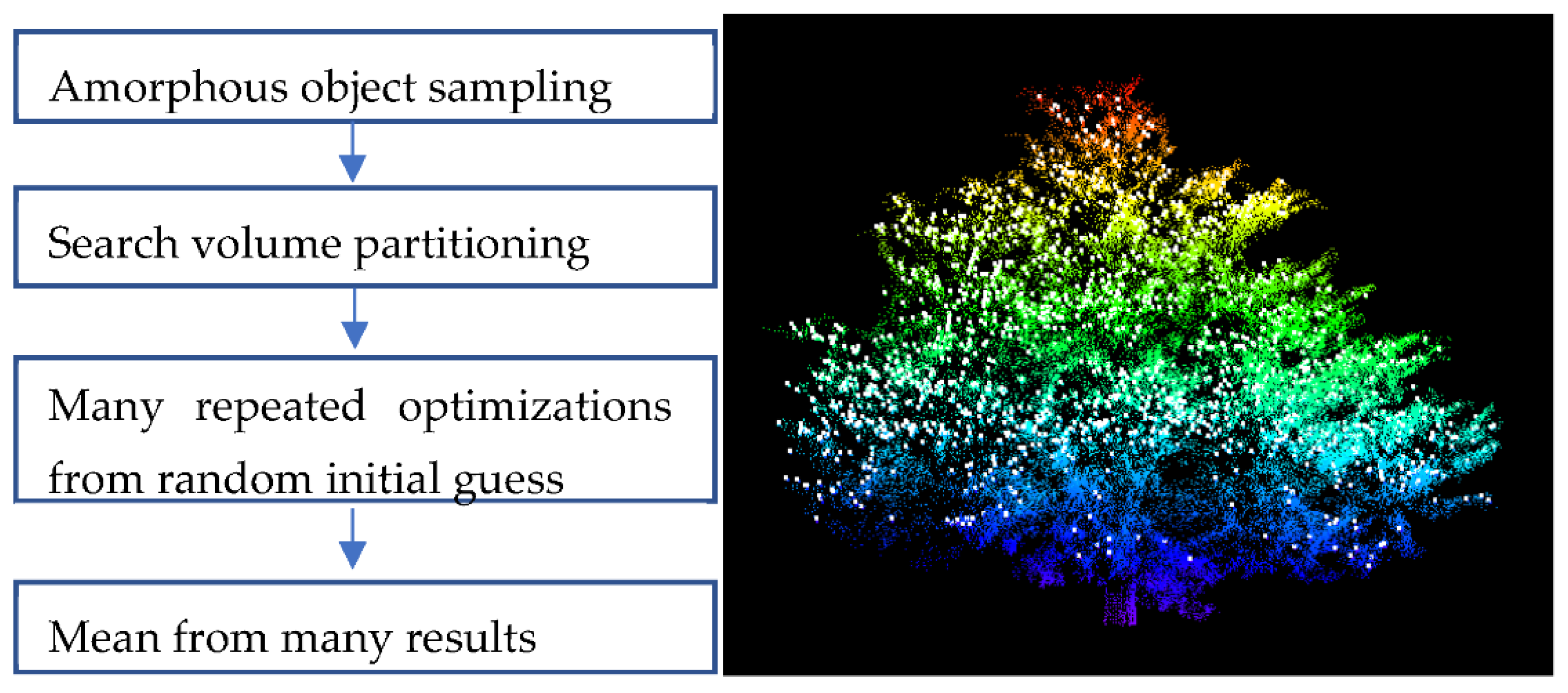Figure 1 describes a brief flowchart of the method using an amorphous object as well as a sampled point cloud from an amorphous object (tree) as an example. The very high-resolution reference TLS point cloud is shown in color (relatively colored by z), and the low-resolution airborne point cloud is shown in larger white dots.

An example of the optimization process (showing just one out of 50 repetitions) details how the three parameters (∆x, ∆y, ∆z) are adjusted at each iteration step and how they converged to a local minima vector in the upper plot in Figure 2. The lower plot shows how the associated objective function converges at around the 40th iteration to a minimized error, which is the sum of squared distances from all 5000 airborne lidar points of the tree.

2.4. Optimal Search Volume

Because the calculation of the objective function is basically a brute-force method in its native form, setting up an optimal point cloud search volume allows a faster implementation than blindly searching through the entire point cloud. Search volume is a function of the pre-selected point cloud corresponding to each data point cloud. A small volume of reference point cloud is assigned to each data point cloud. The search volume partitioning dramatically increases the computation efficiency as expected. Thus, search volume partitioning is an important procedure. Furthermore, use of multi-thread computing or even a graphics processing unit (GPU) will improve with time. However, the volume cannot be too small to allow room for the simplex variation to achieve a convergence. Figure 3 illustrates how the horizontal difference (∆x, ∆y) from 50 repeated optimizations is distributed. The mean of all 50 results is the final estimated difference (∆x, ∆y) between reference point cloud and airborne point cloud data using a single amorphous object. Figure 3 also shows the effect of search volume in the optimization.

The different distributions of repeated solutions depending on the search volume are shown in

Table 1. Dependency of optimized solution based on search volume.

Search Volume	10 cm	15 cm	20 cm	25 cm
Reference/Data	204	581	1187	2006
ComputationTime [relative]	1.0	1.6	3.2	5.1
∆x [m]	0.033	0.055	0.066	0.068
∆y [m]	0.011	0.015	0.016	0.018
∆z [m]	−0.029	−0.049	−0.050	−0.055

. First, the mean ∆x value starts from 3.3 cm to converging near 7 cm means the 10-cm search volume is too small for the simplex to find optimal parameters. Additionally, the improving precision with the increasing search volume provides similar insights. However, in this case the cost is increasing computation time. Increasing from 20 cm to 25 cm does not add substantial benefit but takes much longer to compute. Thus, in this case, the optimal search volume is 20 cm. We reiterate that optimal search volume depends on the specific parameters of the data. The reference to data ratio in Table 1 represents the ratio of points used in the optimization.

2.5. Algorithm Performance Comparison

Although the amorphous object method is mainly developed for any amorphous natural object, it is basically a generic method to evaluate mean 3D deviation between two sets of point clouds. Thus, it can also be applied to a point cloud with a well-defined geometric feature. For example, we extracted an intersection point from three modeled planes using three planes from a high-resolution TLS reference point cloud to create a GCP (Figure 4). Low-resolution large dots are airborne point cloud. There are two sets of three planes with different colors (one in light pink, the other in gray color). Thus, using the two conjugate points, the difference in ∆x, ∆y, and ∆z was estimated as −0.010 m, −0.067 m, and −0.019 m, respectively. The amorphous object method was applied to the same two sets of point cloud data. 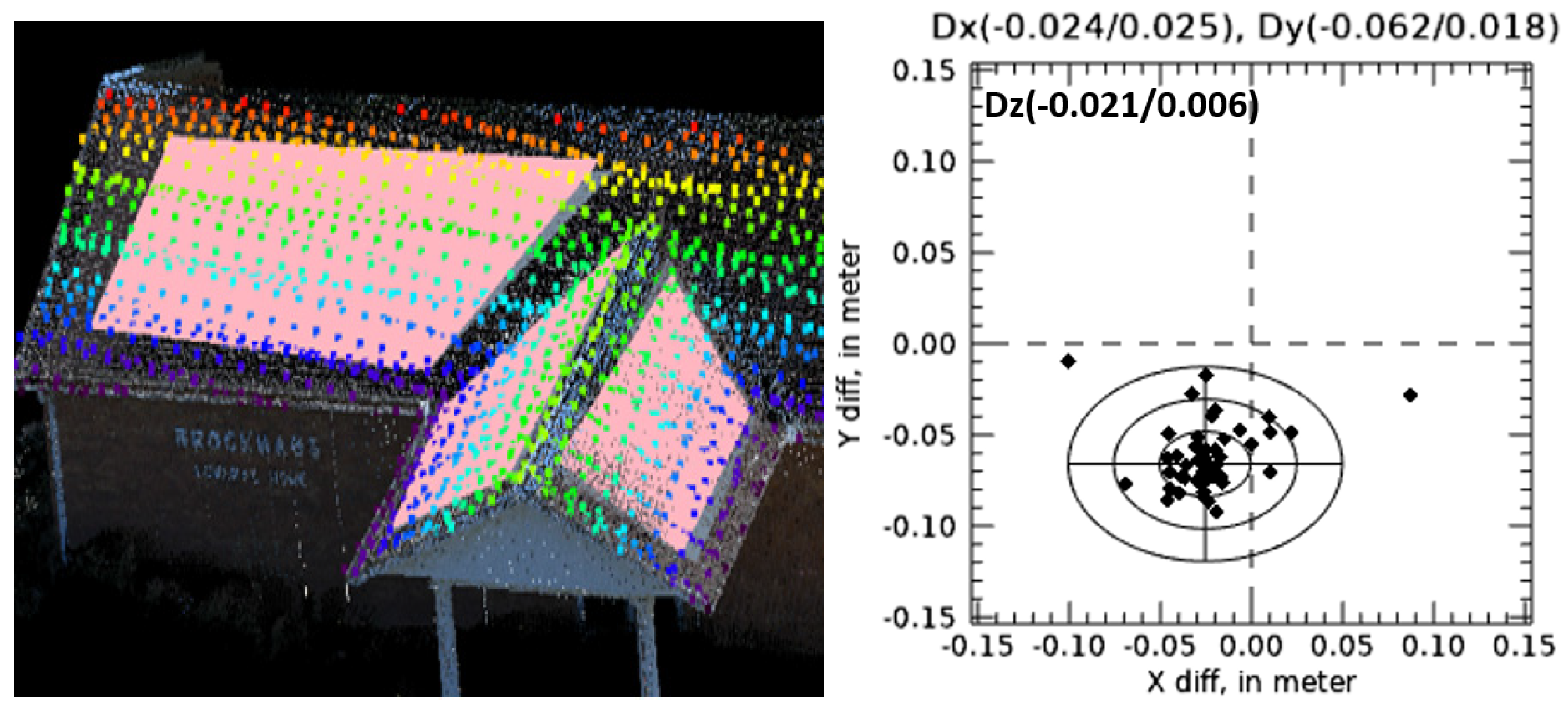The result was estimated as −0.024 m (∆x), −0.062 m (∆y), −0.021 m (∆z) as shown in Figure 5. The estimated difference using the amorphous object method is very similar to the geometric feature method, which is generally considered more robust.

Another example of using this amorphous method on a geometric feature uses a hexagon gazebo, shown in Figure 5. Due to its six-plane geometry, two sets of three-plane point clouds were used, although many more combinations are possible. Using the identical method described above, the difference in ∆x, ∆y, and ∆z was estimated as (−0.031 m, −0.009 m, −0.039 m) for the first three-plane and (−0.025 m, −0.008 m, −0.028 m) for the second three-plane. Since the amorphous method uses the sampled point cloud at the same time, it yields only one difference vector as (−0.034 m, −0.020 m, −0.037 m), as shown in the lower plots in Figure 5. The difference is about 1 cm for all three axes, demonstrating comparable results of the amorphous object method against the robust geometric feature method.

2.6. Applicability to Two-Plane Object

A two-sided roof is the most common built object in the field. However, it is difficult to extract a GCP because two planes do not create an intersection point. One may think the two pitch lines make an intersection point to be used as a GCP; however, the associated uncertainty with the resultant GCP is too high to be of use. That means the external uncertainty associated with the pitch line crossing method is so high that it invalidates proper accuracy assessment.

In comparison, the amorphous method utilizes the entire point cloud, thus it is possible to estimate 3D difference. The result using the two-roof building as shown in Figure 6 yields a difference in ∆x, ∆y, and ∆z of −0.004 cm, −0.010 cm, and −0.042 cm, respectively, and the outcome is comparable to previous results.

3. Results of Accuracy Assessment

The full-scale application of the amorphous object method is to sample ground truth data scattered over a project area, especially in natural systems. In this study we used 108 amorphous objects (trees) for the accuracy assessment of the airborne point cloud. Figure 7 demonstrates how the raw TLS point cloud on the left is sampled for isolated tree objects. The 11 circular voids in the raw TLS point cloud represent the TLS scanning locations. In the right plot of Figure 7, the cleaned and isolated tree point cloud extraction shows single isolated trees, but some objects are the result of merged canopies from multiple trees.

Table 2. Three-dimensional positional differences using the amorphous object method (TLS—airborne data).

Niobrara_Valley_Preserve_Building (14TMN1537, 14TMN1637)
	ID	∆x (m)	∆y (m)	∆z (m)
	1	0.064	0.016	−0.050
	2	0.021	0.041	−0.056
	3	−0.022	0.031	−0.041
	4	0.024	0.054	−0.046
	5	−0.005	0.013	−0.060
	6	−0.006	0.016	−0.059
	7	−0.029	0.004	−0.057
	8	0.008	0.052	−0.048
	9	0.042	0.043	−0.066
	10	0.002	0.022	−0.061
	11	0.014	0.007	−0.066
	12	0.023	0.036	−0.073
	13	0.027	0.037	−0.045
	14	0.017	0.032	−0.049
	15	0.004	0.029	−0.077
	16	0.070	0.084	−0.034
	17	0.061	−0.004	−0.058
	18	−0.013	0.006	−0.044
	19	−0.016	−0.005	−0.030
	20	0.019	−0.035	−0.053
	21	0.016	−0.038	−0.042
	22	0.009	0.039	−0.039
Niobrara_Churches (14TNN7833)
	ID	∆x (m)	∆y (m)	∆z (m)
	1	−0.048	−0.048	−0.040
	2	−0.036	−0.069	−0.017
	3	−0.003	−0.022	−0.025
	4	−0.015	0.011	−0.040
	5	0.010	−0.026	−0.034
	6	−0.003	−0.059	−0.034
	7	0.100	0.009	−0.032
	8	0.015	−0.017	−0.044
	9	0.022	−0.010	−0.026
	10	−0.023	−0.047	−0.034
	11	−0.052	−0.071	−0.042
	12	−0.056	−0.052	−0.082
	13	0	−0.017	−0.024
	14	0.018	−0.019	−0.052
Niobrara_School_Buildings (14TNN7933)
	ID	∆x (m)	∆y (m)	∆z (m)
	1	0	−0.005	−0.037
	2	0.027	0.021	−0.080
	3	−0.016	0.016	−0.043
	4	−0.036	−0.019	−0.020
	5	−0.033	−0.028	−0.030
	6	−0.017	−0.018	−0.028
	7	−0.037	−0.009	−0.044
	8	−0.038	0.005	−0.038
	9	−0.037	0.033	−0.052
	10	−0.048	0.066	−0.043
	11	−0.034	0.036	−0.013
	12	−0.018	−0.008	−0.054
	13	0.019	0.021	−0.043
	14	−0.028	−0.033	−0.022
	15	−0.043	−0.032	−0.038
	16	−0.015	−0.058	−0.036
	17	−0.036	−0.013	−0.037
	18	−0.022	−0.017	−0.023
	19	−0.020	0.003	−0.022
	20	−0.008	−0.025	−0.032
	21	−0.078	−0.006	−0.038
	22	−0.048	−0.014	−0.023
	23	−0.050	0.032	−0.027
Fort_Niobrara_NWR_Out_Building (14TLN7949, 14TLN7950)
	ID	∆x (m)	∆y (m)	∆z (m)
	1	0.014	−0.013	−0.074
	2	0.022	−0.010	−0.065
	3	0.009	−0.033	−0.066
	4	0.026	−0.044	−0.072
	5	0.009	−0.089	−0.067
	6	0.025	0.024	−0.052
	7	0.039	−0.014	−0.051
	8	0.017	−0.025	−0.082
	9	0.040	−0.040	−0.068
	10	0.026	−0.045	−0.079
	11	0.022	−0.073	−0.061
	12	0.009	−0.077	−0.059
	13	0.027	−0.037	−0.039
	14	0.035	−0.001	−0.059
	15	−0.018	−0.060	−0.055
	16	−0.005	−0.081	−0.034
	17	0.006	−0.041	−0.062
Fort_Niobrara_NWR_Visitor_Building (14TLN7949, 14TLN7950)
	ID	∆x (m)	∆y (m)	∆z (m)
	1	−0.002	0.021	−0.033
	2	0.016	−0.022	−0.064
	3	−0.018	−0.003	−0.066
	4	−0.014	0	−0.071
	5	0.006	0.010	−0.084
	6	0.020	−0.019	−0.050
	7	−0.033	−0.001	−0.038
	8	−0.020	−0.014	−0.030
Niobrara_State_Park_Hexagon_Building (14TNN7735)
	ID	∆x (m)	∆y (m)	∆z (m)
	1	0.025	0.018	−0.027
	2	0.023	0.027	−0.031
	3	0.042	0.025	−0.025
	4	0.028	0.086	−0.054
	5	0.017	0.078	−0.062
	6	0.024	0.009	−0.031
	7	0.033	0.018	−0.038
	8	0.047	−0.034	−0.022
	9	0.011	0.052	−0.013
	10	0.005	0.035	−0.012
	11	0.008	0.061	−0.04
Niobrara_State_Park_Pond_Building (14TNN7735)
	ID	∆x (m)	∆y (m)	∆z (m)
	1	0.016	0.026	−0.046
	2	−0.008	0.043	−0.037
	3	−0.015	0.038	−0.030
	4	−0.002	0.014	−0.056
	5	0.023	−0.009	−0.061
	6	−0.047	0.027	−0.021
	7	0.024	−0.010	−0.048
	8	−0.028	0.014	−0.032
	9	−0.008	0.013	−0.036
	10	−0.011	0.011	−0.033
	11	0.029	0.009	−0.017
	12	0.025	0.027	−0.029
	13	0.017	−0.015	−0.047

lists the result of positional differences between the reference point cloud and the airborne data point cloud using the amorphous method, where each result is the result from 50 iterations. Each site ID represents an extracted area of the TLS point cloud data, and the corresponding airborne lidar point cloud tile name is within the parentheses in Table 2.

Using all differences from 108 trees, the final accuracy results of the airborne point cloud are computed as shown in

Table 3. Final accuracy of airborne point cloud using the amorphous object method.

	∆x (m)	∆y (m)	∆z (m)
Mean (m)	−0.001	−0.001	−0.045
RMSE (m)	0.031	0.036	0.017

. Additionally, shown are the horizontal and vertical error distributions in Figure 8. The final uncertainty of the data around 3–4 cm horizontal and 2 cm vertical is an excellent result compared to typical airborne lidar accuracy. Note that USGS QL1 requirement is 10 cm. While the mean vertical error 4.5 cm is not negligibly small, the mean horizontal error is near zero, which is ideal.

4. External Uncertainty

We also derived a general external uncertainty model for the amorphous object method. The external uncertainty is solely dependent on the amorphous object method itself. Modeling external uncertainty should consider several dominant factors that affect the external uncertainty: size of the object, point density of the data, TPU of the lidar sensor, and point density of high-resolution reference system.

4.1. Airborne Lidar Simulator

The four dominant factors mentioned above need to be systematically controlled to investigate how they affect the external uncertainty. Preparing a large number of targets with varying sizes in combination with multiple point density settings and various TPU specifications of the sensors is not a practical research design in terms of feasibility. To test this, we used an airborne lidar simulator created for a companion study [16,23].

A lidar waveform is computed using the laser properties (pulse width, beam divergence angle, and the pulse distribution function), pulse distance determined by sensor altitude and scanner, environmental parameters (absorption and scattering coefficient of the atmosphere), and the 3D geometrical definition of a target. A full waveform solution uses the radiative transfer theory of a laser pulse [24]. The radiative transfer theory is numerically solved for the laser beam irradiance distribution function at a given propagation distance. Two irradiance distribution functions are computed: Irradiance due to the laser beam propagation and irradiance due to the receiver sensitivity propagation. The irradiance distribution function interacts with a target whose geometry is defined in the 3D coordinate system, and the waveform intensity at a given time is obtained by numerically solving a laser interaction governing equation [25].

The second major component of our airborne lidar simulator is the solution of a direct georeferencing equation. A scanner module (scanner type, scan frequency, and the field of view), a global navigation satellite system and strap-down inertial navigation system module for sensor position and orientation, the flight parameters (sensor altitude, flight speed), and the calibration parameters (boresighting and lever-arm) are the essential inputs required to solve a lidar direct georeferencing equation to estimate the 3D position of a laser-target interaction spot.

To model external uncertainty, we designed specific targets for the 3D uncertainty simulation. A tetrahedron/pyramid target was created, and a large array of these pyramid targets were simulated as a surface digital elevation model. As the simulator produces lidar point clouds with various realistic input parameters, the distribution of the point clouds shows spatially inhomogeneous patterns strongly influenced by the roll, pitch, and heading, as well as the scanner type. All these were necessary to simulate realistic situations for the general external uncertainty model development, as the real targets will be placed at a random position, affecting external uncertainty.

4.2. Simulation Design

The discrete values of each factor that were combined as the input parameters for the simulation are listed in

Table 4. Discrete values used in the simulation.

Factors	Discrete Values
Pyramid size [m]	2 × 2 × 2, 3 × 3 × 3, 4 × 4 × 4
Data density [PPSM]	2, 4, 9, 16
Reference density [PPSM]	50, 70, 100, 140, 200, 300, 430, 600
TPU [cm]	3.3, 3.6, 4.0, 4.5, 5.2, 6.0, 7.0, 8.2, 9.4, 10.9

. The point density of high-resolution reference data can easily be much higher, but the maximum simulation range of 600 is set because additional increase does not improve the performance of amorphous method. Although TPU is 3D in nature, the chosen values are assumed to represent overall system performance.

Several selected cases are visualized in the upper plot in Figure 9 regarding size and data density. The TPU values in Figure 9 represent overall sensor performance. The reference white dotted line in the lower plot of Figure 9 represents one pyramid side plane projected to a one-dimensional (1D) line. Thus, the distribution of the points above the line is related to the overall uncertainty (TPU) of a sensor.

The total number of combinations equals 960, which is obtained by multiplying 3, 4, 8, and 10 discrete input values as described in Table 4. Thus, there will be 960 external uncertainties at all three axes. To confirm the uncertainty value was statistically significant and stable, many objects were simulated for each given size and point density as illustrated in Figure 10. In fact, Figure 10 shows only the 5-by-5 pyramid object array created from lidar point cloud simulator to see the details that the point cloud is different for each pyramid. Hundreds of pyramids were created, and each pyramid was reused for optimization multiple times by giving additional random shift. Thus, several thousands of optimizations were performed, and the thousands of optimization results were used to compute one external uncertainty, and this procedure was repeated for all 960 cases.

4.3. External Uncertainty

Figure 11 shows selected examples of estimated external uncertainties on the x-axis (two upper plots) and z-axis (two lower plots). Uncertainties on the y-axis are very similar to the x-axis, as they both form a horizontal external uncertainty. For all plots, the top curve represents the worst sensor in terms of TPU (10.9 cm TPU), and the bottom curve represents the best sensor (3.3 cm TPU). The better sensor (lower curves with small TPU value) has a much smaller external uncertainty. Regardless of the sensor quality (for any TPU value), increasing point density of high-resolution reference data improves the external uncertainty. The most efficient way to display an entire external uncertainty result is to combine all results in a single plot as shown in Figure 12.

All external uncertainties on the x-axis are compiled in Figure 12. Uncertainties are divided into three groups depending on the object size. Unless the object is too small, the amorphous object method is a valid method because even a 2-m object along with high point density reduces external uncertainty to a small enough value. In each size group, increasing point density improves the performance of the amorphous object method. The biggest effect comes from increasing point density of high-resolution reference data, which has the largest gradient (green line) in Figure 12. This is a highly encouraging aspect because the high PPSM of the reference scanner data is easy to achieve. The second biggest effect comes from varying sensor quality (TPU). With all other factors fixed, using a better sensor (smaller TPU) dramatically reduces the external uncertainty of the amorphous object method, as the trend is illustrated along the red line in Figure 12. Using airborne data with larger point density reduces external uncertainty only marginally. Although Figure 12 shows external uncertainties simply listed in a 1D manner and it happened to show an apparent zig-zag pattern, it provides easy-to-understand insights on the effect of each variable in four-dimensional set up. Figure 13 compiles all 3D external uncertainties using dots with different colors without lines to provide a complete picture. A colored dot plot was chosen as a best chart type to avoid chaotic appearance when lines were added.

5. Conclusions

Full 3D accuracy assessment is still not common practice, at least in the mainstream large scale data collection campaigns being conducted today. Although lidar data standard documents clearly state a horizontal accuracy requirement as well as vertical accuracy, surveying many artificial objects with well-defined geometric features is costly compared to the conventional GNSS rover point measurements typically conducted to assess accuracy. Collecting artificial objects to assess accuracy usually involves buildings or other structures. Surveying private buildings is not an option without permission, but even collecting TLS data over public buildings and structures can require permissions to survey. Surveying mostly amorphous objects such as trees and other natural features improves the chance of getting permission, even on private land. The disadvantage of using a ground-based sensor is the difficulty of collecting point cloud in the nadir-viewing perspective, especially on taller structures. Amorphous object scanning is much easier than buildings, which requires careful selection of scan position to avoid self-shadowing. Most of all, the amorphous object method can produce a small external uncertainty, creating a comparable quality accuracy assessment result similar to the more robust geometric feature-based method, but with fewer permission issues. In the example above, in the Niobrara River survey, the horizontal accuracy just over 3 cm is almost the best possible result considering the inherent uncertainty of GNSS system.

The purpose of the extensive simulation was to quantify external uncertainty associated with the amorphous object method, which is modeled in Equation (2). The essential argument regarding this research is, when a certain accuracy assessment technique is suggested, associated external uncertainty must be provided. Thus, any suggested method should be practiced in a manner such that the external uncertainty is not too large because too large external uncertainty will overwhelm the inherent accuracy of the data, thus improper methods would invalidate the accuracy assessment itself. A practical way to use the concept of external uncertainty can be proposed as follows. A lidar data quality guideline can set up a requirement to use a specific accuracy assessment method only if the associated external uncertainty is under a maximum tolerance limit. For example, if the maximum allowed external uncertainty is set to 3 cm, then a horizontal line (red line in Figure 13) as an upper limit can be drawn along 3 cm. Thus, any ground truth and accuracy assessment must find the proper combination of the relevant factors to satisfy the requirement. The easiest solution would be the combination of increasing the point density of reference scanner data and using better quality airborne sensor (smaller TPU) as illustrated in Figure 12. The full 3D accuracy assessment is still challenging and rare. However, once it becomes routine practice, the amorphous object method would be potentially one of the top choices due to its general applicability and robustness, as demonstrated in this research.